Homoclinic Tubes and Chaos in Perturbed Sine-Gordon Equation

Abstract.

In [1], Bernoulli shift dynamics of submanifolds was established in a neighborhood of a homoclinic tube. In this article, we will present a concrete example: sine-Gordon equation under a quasi-periodic perturbation.

1. Introduction

Propagations of nonlinear waves through homogeneous media are often modeled by well-known nonlinear wave equations, for example, sine-Gordon equation. Studies were also drawn to variable media [2] [3] [4]. Variations of the media can speed up, slow down (even stop), or break the wave propagations. Studies have been focused upon such variations of the media, which are localized defects. In the current article, we will study quasi-periodic media. The equation to be studied can be called a quasi-periodically defective sine-Gordon equation. This equation represents a concrete example realizing the theorem proved in [1] [5]. Consequently, existence of a homoclinic tube asymptotic to a torus can be proved, and Bernoulli shift dynamics of tori can be established.

The article is organized as follows: In section 2, we present the formulation of the problem. Section 3 is on an intergable theory. Section 4 is on the existence of a homoclinic tube and chaos.

2. Formulations of the Problem

Consider the sine-Gordon equation under a quasi-periodic perturbation,

(2.1) $$u_{tt}=c^{2}u_{xx}+\sin u+\epsilon[{\mathcal{D}}u+f(t)(\sin u-u)]\ ,$$

which is subject to periodic boundary condition and odd constraint

(2.2) $$u(t,x+2\pi)=u(t,x)\ ,\quad u(t,-x)=-u(t,x)\ ,$$

where $u$ is a real-valued function of two real variables $t\geq 0$ and $x$, c is a parameter, $\frac{1}{2}<c<1$, $\epsilon$ is a small parameter, $\epsilon\geq 0$, ${\mathcal{D}}$ is a dissipative operator

$${\mathcal{D}}u=-au_{t}+bu_{txx}\ ,\quad a\geq 0\ ,\quad b\geq 0\ ,$$

and $f(t)$ is quasi-periodic with a basis of frequencies $\omega_{1},\cdots,\omega_{N}$,

$$f(t)=\sum_{n=1}^{N}a_{n}\cos[\theta_{n}(t)]\ ,\quad\theta_{n}(t)=\omega_{n}t+\theta_{n}^{0}\ ,$$

where $a_{n}$ and $\theta_{n}^{0}$ are parameters. The above system is invariant under the transform $u\rightarrow-u$. On the other hand, the odd constraint prohibits the transform $u\rightarrow u+2\pi$. Equation (2.1) is equivalent to the following system

(2.3) $$\left(\begin{array}[]{c}u\cr v\cr\end{array}\right)_{t}=L\left(\begin{array}[]{c}u\cr v\cr\end{array}\right)+\left(\begin{array}[]{c}0\cr\sin u+\epsilon f(t)(\sin u-u)\cr\end{array}\right)\ ,$$

where

$$L\left(\begin{array}[]{c}u\cr v\cr\end{array}\right)=\left(\begin{array}[]{c}v\cr c^{2}u_{xx}-\epsilon av+\epsilon bv_{xx}\cr\end{array}\right)\ .$$

When $\epsilon=0$, $L$ generates a $C_{0}$ semi-group on $H^{1}\times L^{2}$ (the Sobolev spaces $H^{1}$ and $H^{0}=L^{2}$ on $[0,2\pi]$), and the domain of $L$ is $H^{2}\times H^{1}$. When $\epsilon\neq 0$, $L$ still generates a $C_{0}$ semi-group on $H^{1}\times L^{2}$, but if $b\neq 0$, then the domain of $L$ is $H^{2}\times H^{2}$. Since the nonlinear term in (2.3) is uniformly Lipschitz, (2.3) is globally well-posed in $C([0,\infty),H^{1}\times L^{2})$. That is, for any $(u_{0},v_{0})\in H^{1}\times L^{2}$, there exists a unique mild solution $(u(t),v(t))\in C([0,\infty),H^{1}\times L^{2})$ such that $(u(0),v(0))=(u_{0},v_{0})$. One can introduce the evolution operator $F^{t}$ as $(u(t),v(t))=F^{t}(u_{0},v_{0})$. If $b=0$, $F^{t}$ is defined for all $t\in\mathbb{R}$, and for any fixed $t$, $F^{t}$ is a $C^{\infty}$ diffeomorphism. For a classical reference, see [6].

3. Integrable Theory

When $\epsilon=0$, equation (2.1) reduces to the well-known sine-Gordon equation

(3.1) $$u_{tt}=c^{2}u_{xx}+\sin u\ ,$$

which is integrable through the Lax pair

(3.2) $$\psi_{x} = B\psi\ ,$$

(3.3) $$\psi_{t} = A\psi\ ,$$

where

$$B=\frac{1}{c}\left(\begin{array}[]{lr}\frac{i}{4}(cu_{x}+u_{t})&\frac{1}{16\lambda}e^{iu}+\lambda\cr\cr-\frac{1}{16\lambda}e^{-iu}-\lambda&-\frac{i}{4}(cu_{x}+u_{t})\cr\end{array}\right)\ ,$$

$$A=\left(\begin{array}[]{lr}\frac{i}{4}(cu_{x}+u_{t})&-\frac{1}{16\lambda}e^{iu}+\lambda\cr\cr\frac{1}{16\lambda}e^{-iu}-\lambda&-\frac{i}{4}(cu_{x}+u_{t})\cr\end{array}\right)\ .$$

The Lax pair (3.2)-(3.3) possesses a symmetry.

Lemma 3.1.

If $\psi=\left(\begin{array}[]{c}\psi_{1}\cr\psi_{2}\cr\end{array}\right)$ solves the Lax pair (3.2)-(3.3) at $(\lambda,u)$, then $\left(\begin{array}[]{c}\overline{\psi_{2}}\cr\cr\overline{\psi_{1}}\cr\end{array}\right)$ solves the Lax pair (3.2)-(3.3) at $(-\bar{\lambda},u)$.

There is a Darboux transformation for the Lax pair (3.2)-(3.3).

Theorem 3.2 (Darboux Transformation I).

Let

$$U = u+2i\ln\left[\frac{i\phi_{2}}{\phi_{1}}\right]\ ,$$

(3.6) $$\Psi = \left(\begin{array}[]{lr}-\nu\phi_{2}/\phi_{1}&\lambda\cr-\lambda&\nu\phi_{1}/\phi_{2}\cr\end{array}\right)\psi\ ,$$

where $\phi=\psi|_{\lambda=\nu}$ for some $\nu$, then $\Psi$ solves the Lax pair (3.2)-(3.3) at $(\lambda,U)$.

Often in order to guarantee the reality condition (i.e. $U$ needs to be real-valued), one needs to iterate the Darboux transformation by virtue of Lemma 3.1. The result corresponds to the counterpart of the Darboux transformation for the cubic nonlinear Schrödinger equation [7].

Theorem 3.3 (Darboux Transformation II).

Let

$$U = u+2i\ln\left[\frac{\nu|\phi_{1}|^{2}+\bar{\nu}|\phi_{2}|^{2}}{\bar{\nu}|\phi_{1}|^{2}+\nu|\phi_{2}|^{2}}\right]\ ,$$

$$\Psi = G\psi\ ,$$

where

(3.9) $$G = \left(\begin{array}[]{lr}G_{1}&G_{2}\cr G_{3}&G_{4}\cr\end{array}\right)\ ,$$

$$G_{1} = |\nu|^{2}\frac{\nu|\phi_{1}|^{2}+\bar{\nu}|\phi_{2}|^{2}}{\bar{\nu}|\phi_{1}|^{2}+\nu|\phi_{2}|^{2}}-\lambda^{2}\ ,$$

$$G_{2} = \frac{\lambda(\nu^{2}-\bar{\nu}^{2})\phi_{1}\overline{\phi_{2}}}{\bar{\nu}|\phi_{1}|^{2}+\nu|\phi_{2}|^{2}}\ ,$$

$$G_{3} = \frac{\lambda(\nu^{2}-\bar{\nu}^{2})\overline{\phi_{1}}\phi_{2}}{\nu|\phi_{1}|^{2}+\bar{\nu}|\phi_{2}|^{2}}\ ,$$

$$G_{4} = |\nu|^{2}\frac{\bar{\nu}|\phi_{1}|^{2}+\nu|\phi_{2}|^{2}}{\nu|\phi_{1}|^{2}+\bar{\nu}|\phi_{2}|^{2}}-\lambda^{2}\ ,$$

and $\phi=\psi|_{\lambda=\nu}$ for some $\nu$, then $\Psi$ solves the Lax pair (3.2)-(3.3) at $(\lambda,U)$.

Proof: Let $\phi$ be an eigenfunction solving the Lax pair (3.2)-(3.3) at $(\lambda,u)$. With ($\phi,\nu,u$), the Darboux transformation given in Theorem 3.2 leads to

(3.10) $$\tilde{U} = u+2i\ln\left[\frac{i\phi_{2}}{\phi_{1}}\right]\ ,$$

(3.13) $$\tilde{\Psi} = \left(\begin{array}[]{lr}-\nu\phi_{2}/\phi_{1}&\lambda\cr-\lambda&\nu\phi_{1}/\phi_{2}\cr\end{array}\right)\psi\ .$$

By Lemma 3.1, $\hat{\phi}=\left(\begin{array}[]{c}\overline{\phi_{2}}\cr\cr\overline{\phi_{1}}\cr\end{array}\right)$ solves the Lax pair (3.2)-(3.3) at $(-\bar{\nu},u)$. Hence,

$$\hat{\Phi}=\left(\begin{array}[]{lr}-\nu\phi_{2}/\phi_{1}&-\bar{\nu}\cr\bar{\nu}&\nu\phi_{1}/\phi_{2}\cr\end{array}\right)\hat{\phi}$$

solves the Lax pair (3.2)-(3.3) at $(-\bar{\nu},\tilde{U})$. With ($\hat{\Phi},-\bar{\nu},\tilde{U}$), the Darboux transformation given in Theorem 3.2 leads to the expressions given in the current theorem. Q.E.D.

Focusing upon the spatial part (3.2) of the Lax pair, one can develop a complete Floquet theory. Let $M(x)$ be the fundamental matrix of (3.2), $M(0)=I$ ($2\times 2$ identity matrix), then the Floquet discriminant is given as

$$\Delta=\ \mbox{trace}\ M(2\pi)\ .$$

The Floquet spectrum is given by

$$\sigma=\{\lambda\in\mathbb{C}\ |\ -2\leq\Delta(\lambda)\leq 2\}\ .$$

Periodic and anti-periodic points $\lambda^{\pm}$ (which correspond to periodic and anti-periodic eigenfunctions respectively) are defined by

$$\Delta(\lambda^{\pm})=\pm 2\ .$$

A critical point $\lambda^{(c)}$ is defined by

$$\frac{d\Delta}{d\lambda}(\lambda^{(c)})=0\ .$$

A multiple point $\lambda^{(m)}$ is a periodic or anti-periodic point which is also a critical point. The algebraic multiplicity of $\lambda^{(m)}$ is defined as the order of the zero of $\Delta(\lambda)\pm 2$ at $\lambda^{(m)}$. When the order is $2$, we call the multiple point a double point, and denote it by $\lambda^{(d)}$. The order can exceed $2$. The geometric multiplicity of $\lambda^{(m)}$ is defined as the dimension of the periodic or anti-periodic eigenspace at $\lambda^{(m)}$, and is either $1$ or $2$.

Counting lemmas for $\lambda^{\pm}$ and $\lambda^{(c)}$ can be established similarly as in [7]. As a result, there exist sequences $\{\lambda^{\pm}_{j}\}$ and $\{\lambda^{(c)}_{j}\}$. An important sequence of invariants $F_{j}$ of the sine-Gordon equation can be defined by

$$F_{j}(u,u_{t})=\Delta(\lambda^{(c)}_{j}(u,u_{t}),u,u_{t})\ .$$

If $\{\lambda^{(c)}_{j}\}$ is a simple critical point of $\Delta$, then

$$\frac{\partial F_{j}}{\partial w}=\frac{\partial\Delta}{\partial w}\bigg{|}_{\lambda=\lambda^{(c)}_{j}}\ ,\quad w=u,u_{t}\ .$$

As a function of three variables, $\Delta=\Delta(\lambda,u,u_{t})$ has the partial derivatives given by Bloch functions $\psi^{\pm}$ (i.e. $\psi^{\pm}(x)=e^{\pm\Lambda x}\tilde{\psi}^{\pm}(x)$, where $\tilde{\psi}^{\pm}$ are periodic in $x$ of period $2\pi$, and $\Lambda$ is a complex constant):

$$\frac{\partial\Delta}{\partial u} = \frac{-i}{16\lambda c}\frac{\sqrt{\Delta^{2}-4}}{W(\psi^{+},\psi^{-})}\bigg{[}4\lambda c\partial_{x}(\psi^{+}_{1}\psi^{-}_{2}+\psi^{+}_{2}\psi^{-}_{1})+e^{-iu}\psi^{+}_{1}\psi^{-}_{1}-e^{iu}\psi^{+}_{2}\psi^{-}_{2}\bigg{]}\ ,$$

$$\frac{\partial\Delta}{\partial u_{t}} = \frac{i}{4c}\frac{\sqrt{\Delta^{2}-4}}{W(\psi^{+},\psi^{-})}\bigg{[}\psi^{+}_{1}\psi^{-}_{2}+\psi^{+}_{2}\psi^{-}_{1}\bigg{]}\ ,$$

$$\frac{\partial\Delta}{\partial\lambda} = \frac{-1}{c}\frac{\sqrt{\Delta^{2}-4}}{W(\psi^{+},\psi^{-})}\int_{0}^{2\pi}\bigg{[}\bigg{(}\frac{1}{16\lambda^{2}}e^{iu}-1\bigg{)}\psi^{+}_{2}\psi^{-}_{2}+\bigg{(}\frac{1}{16\lambda^{2}}e^{-iu}-1\bigg{)}\psi^{+}_{1}\psi^{-}_{1}\bigg{]}dx\ ,$$

where ${W(\psi^{+},\psi^{-})}=\psi^{+}_{1}\psi^{-}_{2}-\psi^{+}_{2}\psi^{-}_{1}$ is the Wronskian. Of course, the sine-Gordon equation can be written in the Hamiltonian form

$$u_{t}=\frac{\partial H}{\partial v}\ ,\quad v_{t}=-\frac{\partial H}{\partial u}\ ,$$

where the Hamiltonian is given by

$$H=\int_{0}^{2\pi}\bigg{[}\frac{1}{2}(v^{2}+c^{2}u_{x}^{2})+\cos u\bigg{]}dx\ .$$

It turns out that $F_{j}$’s provide the perfect Melnikov vectors rather than the Hamiltonian or other invariants [7].

$u=0$ is a fixed point of the sine-Gordon equation. Linearization of the sine-Gordon equation at $u=0$ leads to

$$u_{tt}=c^{2}u_{xx}+u\ .$$

Let $u=\sum_{k=1}^{\infty}u_{k}^{0}e^{\Omega_{k}t}\sin kx$, $u_{k}^{0}$ and $\Omega_{k}$ are constants, then

$$\Omega_{k}=\pm\sqrt{1-c^{2}k^{2}}\ ,\quad k=1,2\cdots.$$

Since $1/2<c<1$, only $k=1$ is an unstable mode, the rest modes are neutrally stable. The corresponding nonlinear unstable foliation can be represented through the Darboux transformation given in Theorem 3.3. When $u=0$, the Bloch functions of the Lax pair (3.2)-(3.3) are

$$\psi^{\pm}=e^{\pm i(\kappa x+\omega t)}\left(\begin{array}[]{c}1\cr\pm i\cr\end{array}\right)\ ,$$

where $\kappa=\frac{1}{c}(\lambda+\frac{1}{16\lambda})$ and $\omega=\lambda-\frac{1}{16\lambda}$. Thus,

$$\lambda=\frac{1}{2}\bigg{[}\kappa c\pm\sqrt{(\kappa c)^{2}-\frac{1}{4}}\bigg{]}\ .$$

The Floquet discriminant is given by

$$\Delta=2\cos(2\pi\kappa)\ .$$

The spectral data are depicted in Figure 1.

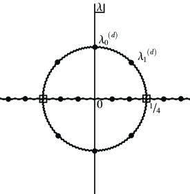
Figure 1. Floquet spectrum of the Lax pair at $u=0$, $\bullet$ double point, $\square$ critical point.

Noticing that the Darboux transformation in Theorem 3.3 depends upon quadratic products of eigenfunctions, one realizes that $\phi$ should be chosen at $\kappa=\frac{1}{2}$ and $\nu=\frac{1}{4}[c+i\sqrt{1-c^{2}}]$. $\nu$ is a complex double point, $\nu=\lambda_{1}^{(d)}$ in Figure 1. (It turns out that for other soliton equations , e.g. Davey-Stewartson II equation [8], $\nu$ may not be a double point.) The wise choice for $\phi$ is

$$\phi=\sqrt{\frac{c_{+}}{c_{-}}}\phi^{+}+\sqrt{\frac{c_{-}}{c_{+}}}\phi^{-}\ ,$$

where

$$\phi^{\pm}=e^{\pm i\frac{1}{2}x\mp\frac{\sigma}{2}t}\left(\begin{array}[]{c}1\cr\pm i\cr\end{array}\right)\ ,\quad\sigma=\sqrt{1-c^{2}}\ ,$$

and $c_{\pm}$ are arbitrary complex constants. Let

$$\frac{c_{+}}{c_{-}}=e^{\rho+i\theta}\ ,\quad\tau=\sigma t-\rho\ ,\quad\xi=x+\theta\ ,$$

then

$$\phi=2\left(\begin{array}[]{c}\cosh\frac{\tau}{2}\cos\frac{\xi}{2}-i\sinh\frac{\tau}{2}\sin\frac{\xi}{2}\cr-\cosh\frac{\tau}{2}\sin\frac{\xi}{2}-i\sinh\frac{\tau}{2}\cos\frac{\xi}{2}\cr\end{array}\right)\ .$$

The Darboux transformation in Theorem 3.3 leads to

(3.14) $$U=\pm 4\vartheta\ ,\quad\vartheta=\arctan\bigg{[}\frac{\sigma}{c}\ \mbox{sech}\tau\sin x\bigg{]}\ ,\quad\vartheta\in(-\frac{\pi}{2},\frac{\pi}{2})\ ,$$

corresponding to $\theta=\pm\frac{\pi}{2}$ (which in turn corresponds to the $U\rightarrow-U$ symmetry). Notice that

$$\mbox{det}\ G=(\lambda^{2}-\nu^{2})(\lambda^{2}-\bar{\nu}^{2})\ ,$$

L’Hospital’s rule implies that

$$\lim_{\lambda\rightarrow\nu}\frac{\sqrt{\Delta^{2}-4}}{W(\Psi^{+},\Psi^{-})}=\frac{\sqrt{\Delta(\nu)\Delta^{\prime\prime}(\nu)}}{2\nu(\nu^{2}-\bar{\nu}^{2})W(\phi^{+},\phi^{-})}\ .$$

Moreover,

(3.18) $$\Phi^{\pm} = G\phi^{\pm}=\pm e^{\mp(\frac{\rho}{2}+i\frac{\theta}{2})}\nu(\nu^{2}-\bar{\nu}^{2})W(\phi^{+},\phi^{-})$$

$$\times\left(\begin{array}[]{c}\frac{-\overline{\phi_{2}}}{\bar{\nu}|\phi_{1}|^{2}+\nu|\phi_{2}|^{2}}\cr\cr\frac{\overline{\phi_{1}}}{\nu|\phi_{1}|^{2}+\bar{\nu}|\phi_{2}|^{2}}\cr\end{array}\right)\ .$$

Finally,

(3.19) $$\frac{\partial F_{1}}{\partial u_{t}}\bigg{|}_{u=U} = \frac{\pi\sigma^{2}}{\sqrt{2}c}\ \mbox{sech}\tau[c^{2}+\sigma^{2}\ \mbox{sech}^{2}\tau\sin^{2}x]^{-1}$$

$$\times[\pm\tanh\tau\sin x\mp i\cos x]\ ,$$

corresponding to $\theta=\pm\frac{\pi}{2}$. The real part of (3.19) is the Melnikov vector.

4. Existence of a Homoclinic Tube and Chaos

The defective sine-Gordon equation (2.1) can be related to an autonomous system by introducing extra phase variables $\theta=(\theta_{1},\cdots,\theta_{N})$,

(4.1) $$u_{tt}=c^{2}u_{xx}+\sin u+\epsilon[{\mathcal{D}}u+f(\theta_{1},\cdots,\theta_{N})(\sin u-u)]\ ,$$

(4.2) $$\frac{d\theta_{n}}{dt}=\omega_{n}\ ,\quad(n=1,\cdots,N)\ .$$

For any $\theta^{0}$, solving (4.2), equation (4.1) becomes (2.1).

$u=0$ corresponds to a $N$-torus denoted by $\tilde{S}$. Linearization at $u=0$ leads to

$$u_{tt}=c^{2}u_{xx}+u+\epsilon{\mathcal{D}}u\ ,$$

$$\frac{d\theta_{n}}{dt}=\omega_{n}\ ,\quad(n=1,\cdots,N)\ .$$

Thus $u=0$ corresponds to a normally hyperbolic $N$-torus with one unstable mode (since $1/2<c<1$), when $\epsilon>0$. Proofs of the following invariant manifold theorem have become standard after the works [9] [10].

Theorem 4.1.

The $N$-torus $\tilde{S}$ has an ($N+1$)-dimensional $C^{m}$ ($m\geq 3$) center-unstable manifold $W^{cu}$ and a $1$-codimensional $C^{m}$ center-stable manifold $W^{cs}$ in the phase space $(u,u_{t},\theta)\in H^{1}\times L^{2}\times\mathbb{T}^{N}$. $W^{cu}\cap W^{cs}=\tilde{S}$. $W^{cu}$ is $C^{1}$ in $\epsilon$ for $\epsilon\in[0,\epsilon_{0})$ and some $\epsilon_{0}>0$. When $b\neq 0$, for $(u,u_{t})\in H^{2}\times H^{2}$, $W^{cs}$ is $C^{1}$ in $\epsilon$ for $\epsilon\in[0,\epsilon_{0})$. When $b=0$, $W^{cs}$ is always $C^{1}$ in $\epsilon$ for $\epsilon\in[0,\epsilon_{0})$. Inside $W^{cu}$ and $W^{cs}$ respectively, there are a $C^{m}$ invariant family of $1$-dimensional $C^{m}$ unstable fibers $\{{\mathcal{F}}^{u}(\theta):\ \theta\in\tilde{S}\}$ and a $C^{m}$ invariant family of $C^{m}$ stable fibers $\{{\mathcal{F}}^{s}(\theta):\ \theta\in\tilde{S}\}$, such that

$$W^{cu}=\bigcup_{\theta\in\tilde{S}}{\mathcal{F}}^{u}(\theta)\ ,\quad W^{cs}=\bigcup_{\theta\in\tilde{S}}{\mathcal{F}}^{s}(\theta)\ .$$

There are positive constants $\kappa_{u}=\frac{1}{2}\sqrt{1-c^{2}}$, $\kappa_{s}=\frac{1}{4}\epsilon(a+b)$, and $C$ such that

$$\|F^{t}(q^{-})-F^{t}(\theta)\| \leq Ce^{\kappa_{u}t}\|q^{-}-\theta\|\ ,\quad\forall t\in(-\infty,0]\ ,$$

$$\forall\theta\in\tilde{S}\ ,\quad\forall q^{-}\in{\mathcal{F}}^{u}(\theta)\ ,$$

$$\|F^{t}(q^{+})-F^{t}(\theta)\| \leq Ce^{-\kappa_{s}t}\|q^{+}-\theta\|\ ,\quad\forall t\in[0,+\infty)\ ,$$

$$\forall\theta\in\tilde{S}\ ,\quad\forall q^{+}\in{\mathcal{F}}^{s}(\theta)\ ,$$

$$\|F^{t}(\theta^{+})-F^{t}(\theta^{-})\| \leq C\|\theta^{+}-\theta^{-}\|\ ,\quad\forall t\in(-\infty,+\infty)\ ,$$

$$\forall\theta^{+},\theta^{-}\in\tilde{S}\ ,$$

where $F^{t}$ is the evolution operator of (4.1)-(4.2).

In terms of the original setting (2.1), ${\mathcal{F}}^{u}(\theta)$ and ${\mathcal{F}}^{s}(\theta)$ are the unstable and stable manifolds of the fixed point $u=0$, which are $C^{m}$ smooth in $\theta^{0}$. As shown in [9] [10], to the leading order, the signed distance between ${\mathcal{F}}^{u}(\theta)$ and ${\mathcal{F}}^{s}(\theta)$ (which is a certain coordinate difference) is given by the Melnikov integral

$$M=\int_{-\infty}^{+\infty}\int_{0}^{2\pi}\bigg{\{}\frac{\partial F_{1}}{\partial u_{t}}\bigg{[}{\mathcal{D}}u+f(t)(\sin u-u)\bigg{]}\bigg{\}}_{u=U}dxdt\ ,$$

where $U$ is given in (3.14) and $\frac{\partial F_{1}}{\partial u_{t}}|_{u=U}$ is given in (3.19). The signed distance between ${\mathcal{F}}^{u}(\theta)$ and ${\mathcal{F}}^{s}(\theta)$ is $C^{m}$ ($m\geq 3$) in $\theta^{0}$. The zero of the Melnikov integral and implicit function theorem imply the following theorem, for detailed arguments, see [9] [10].

Theorem 4.2.

If $b\neq 0$, there is a region for $(a,b)$ in $\mathbb{R}^{+}\times\mathbb{R}^{+}$, or if $b=0$, there is a region for $a$ in $\mathbb{R}^{+}$, such that $W^{cu}$ and $W^{cs}$ intersect into a $N$-dimensional $C^{m}$ ($m\geq 3$) homoclinic tube $\hat{S}$ asymptotic to the $N$-torus $\tilde{S}$.

Additional remarks for the proof of the theorem are that the size of ${\mathcal{F}}^{s}(\theta)$ is of order ${\mathcal{O}}(\sqrt{\epsilon})$ since the nonlinear term in (2.1) is cubic. Therefore, the so-called second measurement in [9] [10] is not needed.

The rest of this article only deals with the case $b=0$. The Poincaré period map $F$ determined by setting $\theta_{1}=2n\pi$ has the homoclinic tube $\xi=(\cdots S_{-1}S_{0}S_{1}\cdots)$ which is asymptotic to the ($N-1$)-torus $S$ obtained from $\tilde{S}$ by setting $\theta_{1}=0$. $S_{0}$ is a $C^{m}$ ($N-1$)-torus as a result of the smoothness of the signed distance with respect to $\theta^{0}$, and $S_{j}=F^{j}S_{0}$, $\forall j\in\mathbb{Z}$. The rest of Assumption (A1) in [1] can be verified by noticing that the decay rates in (4.1)-(4.1) are uniform with respect to $\theta$, and the fact that ${\mathcal{F}}^{u}(\theta)$ and ${\mathcal{F}}^{s}(\theta)$ are the unstable and stable manifolds of the fixed point $u=0$ of (2.1). Since $S$ is a finite-dimensional torus, $\xi\cup S$ is compact, thus Assumption (A2) in [1] is also satisfied. Therefore, we have the following theorem.

Theorem 4.3 (Chaos Theorem).

When $b=0$, there is a Cantor set $\Xi$ of tori which is invariant under the iterated Poincaré map $F^{2K+1}$ for some $K$. The action of $F^{2K+1}$ on $\Xi$ is topologically conjugate to the action of the Bernoulli shift on two symbols $0$ and $1$.

Acknowledgement: I would like to thank Brenda Frazier for artist work.

References

• [1] Y. Li, Chaos and shadowing aound a homoclinic tube, Accepted, Abstract and Applied Analysis (2003).
• [2] F. Zhang, Y. Kivshar, L. Vazquez, Resonant kink-impurity interactions in the sine-Gordon model, Phys. Rev. A 45 (1992), 6019.
• [3] R. Goodman, R. Slusher, M. Weinstein, Stopping light on a defect, J. Opt. Soc. Am. B (2001).
• [4] X. Cao, B. Malomed, Soliton-defect collisions in the nonlinear Schrödinger equation, Phys. Lett. A206, No.3-4 (1995), 177.
• [5] Y. Li, Chaos and shadowing lemma for autonomous systems of infinite dimensions, Submitted, available at: http://xxx.lanl.gov/abs/nlin/0203024, or http://www.math.missouri.edu/~cli (2003).
• [6] A. Pazy, Semigroups of Linear Operators and Applications to Partial Differential Equations, Springer-Verlag, Applied Mathematical Sciences, vol.44, 1983
• [7] Y. Li, D. McLaughlin, Morse and Melnikov functions for NLS PDEs, Comm. Math. Phys.162, no. 1 (1994), 175.
• [8] Y. Li, Bäcklund-Darboux transformations and Melnikov analysis for Davey-Stewartson II equations, J. Nonlinear Sci. 10, no.1 (2000), 103.
• [9] Y. Li et al., Persistent homoclinic orbits for a perturbed nonlinear Schrödinger equation, Comm. Pure Appl. Math. 49, no. 11 (1996), 1175.
• [10] Y. Li, Persistent homoclinic orbits for nonlinear Schrödinger equation under singular perturbation, Submitted, available at: http://xxx.lanl.gov//abs/math.AP/0106194, or http://www.math.missouri.edu/~cli (2003).