Multi-frequency Craik-Criminale solutions of the Navier-Stokes equations

Abstract

An exact Craik-Criminale (CC) solution to the incompressible Navier-Stokes (NS) equations describes the instability of an elliptical columnar flow interacting with a single Kelvin wave. These CC solutions are extended to allow multi-harmonic Kelvin waves to interact with any exact “base” solution of the NS equations. The interaction is evaluated along an arbitrarily chosen flowline of the base solution, so exact nonlinear instability in this context is locally convective, rather than absolute. Furthermore, an iterative method called “WKB-bootstrapping” is introduced which successively adds Kelvin waves with incommensurate phases to the extended CC solutions. This is illustrated by constructing an extended CC solution consisting of several Kelvin waves with incommensurate phases interacting with an elliptical columnar flow.

1 Introduction

Craik & Criminale (1986) showed formally that the sum of a base flow that is linear in the spatial coordinates and a single traveling wave is a global solution of the incompressible Navier-Stokes (NS) equations on an unbounded spatial domain. Although this fact was known in certain specific cases (see, for example, (Chandrasekhar, 1961, pp. 85-86)), it was Craik & Criminale who formalized the general framework. This discovery provided an exact nonlinear interpretation of elliptic instability, the resonant mechanism by which vortex stretching creates three-dimensional instabilities in swirling two-dimensional flows Bayly (1986). This nonlinear interpretation of elliptic instability also holds when additional physics such as buoyancy Miyazaki & Fukumoto (1992), rotation Craik (1989); Miyazaki (1993); Bayly et al. (1996) and magnetic fields Craik (1988) are included. Most recently, elliptic instability has been used to study the effects of turbulence models Cambon et al. (1994); Fabijonas & Holm (2003a, b). Elliptic instability and its interpretation using the Craik-Criminale (CC) solutions were recently reviewed by Kerswell (2002).

A second equally ground-breaking body of work related to the CC class of solutions is Lifschitz’s WKB-like stability method for fluid mechanics known as the Geometrical Optics Stability Method (GOSM) Lifschitz & Hameiri (1991); Lifschitz (1994). The method linearizes the perturbation equations about the unperturbed flow and examines the evolution of a high-frequency infinitesimal wavepacket in a Lagrangian reference frame which moves with the unperturbed flow. The power of this method is its insensitivity to the unperturbed flow’s global geometry and time dependence. Remarkably, the equations governing the nonzero leading order terms of GOSM coincide with those for CC solutions. This coincidence motivates the present paper.

This paper bridges the gap between GOSM and CC solutions by extending the CC class of exact nonlinear solutions of the NS equations in two stages. First, we show that the CC construction method works when a Kelvin wave together with any number of its harmonics interacts with any exact solution of the nonlinear NS equations, provided the interaction is evaluated along some arbitrarily chosen flowline of the base solution. This extension of the CC construction method changes its interpretation from absolute instability to locally convective instability Huerre & Monkewitz (1990). Second, we introduce an iterative method called “WKB-bootstrapping” which constructs extended CC solutions interacting with additional traveling waves whose phases are incommensurate. These are multi-frequency CC solutions. (The phrase “incommensurate phases” will be explicitly defined in Eq. (15).) The WKB-bootstrapping algorithm allows Kelvin waves with incommensurate phases to be added to the base flow one at a time. The power of this method is illustrated by deriving the exact solution for nonlinear instability of an elliptical columnar flow that is interacting with several traveling Kelvin waves whose phases are incommensurate. Also, a steady circular columnar flow interacting with a single Kelvin wave is found to be critically stable. That is, either perturbing the streamline to introduce eccentricity, or adding multiple traveling waves with incommensurate phases will yield Kelvin waves with exponentially growing amplitudes.

2 Craik-Criminale solutions for generalized base flows

We consider the NS equations in a coordinate system rotating about the $z-$axis with angular velocity $\mathbf{\Omega}=\Omega{\mathbf{\hat{e}}_{z}}$:

$$\partial_{t}{\mathbf{u}}+{{\mathbf{u}}}\cdot{\nabla}{\mathbf{u}}+2\mathbf{\Omega}\times{\mathbf{u}}+\nabla p=\nu\Delta{\mathbf{u}}\,.$$ (1)

Here ${\nabla}\cdot{{\mathbf{u}}}=0$, where ${\mathbf{u}}$ is a velocity field, $p$ is the pressure, and $\nu$ is the kinematic viscosity. Let ${\mathbf{U}}$ be any exact solution to Eq. (1) with corresponding pressure $P$. Consider a new exact solution of the form ${\mathbf{u}}={\mathbf{U}}+{\mathbf{U}}^{\prime}$, $p=P+P^{\prime}$. In the analysis of nonlinear instability to follow, we shall refer to ${\mathbf{U}}$ as the ‘base’ flow and ${\mathbf{U}}^{\prime}$ as the ‘disturbance.’ We proceed by inserting this additive velocity decomposition into Eq. (1), and using the condition that ${\mathbf{U}}$ is an exact solution, together with the vector identity

$$({{\mathbf{u}}}\cdot{\nabla}){\mathbf{v}}=(\nabla\times{\mathbf{v}})\times{\mathbf{u}}+(\nabla{\mathbf{v}})^{T}\cdot{\mathbf{u}}\,.$$ (2)

Consequently, the nonlinear disturbance dynamics is governed by

$$\partial_{t}{\mathbf{U}}^{\prime}+({{\mathbf{U}}}\cdot{\nabla}){\mathbf{U}}^{\prime}+(\nabla{\mathbf{U}})^{T}\cdot{\mathbf{U}}^{\prime}+({{\mathbf{U}}^{\prime}}\cdot{\nabla}){\mathbf{U}}^{\prime}+\mathbf{\Pi}\times{\mathbf{U}}^{\prime}+\nabla P^{\prime}=\nu\Delta{\mathbf{U}}^{\prime},$$ (3)

and ${\nabla}\cdot{{\mathbf{U}}^{\prime}}=0$. Here, $\mathbf{\Pi}=2\mathbf{\Omega}+\nabla\times{\mathbf{U}}$ denotes the total vorticity of the base flow. We choose the disturbance to consist of a traveling wave and its harmonics of the form

$${\mathbf{U}}^{\prime}=\sum_{m=-\infty}^{\infty}\mu^{|m|}{\mathbf{a}}_{m}(t)e^{im\beta\Phi},\qquad P^{\prime}=\sum_{m=-\infty}^{\infty}i\mu^{|m|}p_{m}(t)e^{im\beta\Phi}.$$ (4)

Here, $\Phi=\Phi(t,{\mathbf{x}})$ is the fundamental phase of the disturbance. In linear analysis, the sum ${\mathbf{U}}+{\mathbf{U}}^{\prime}$ would be a solution to the NS equations linearized about ${\mathbf{U}}$; that is, Eq. (3) with the term quadratic in ${\mathbf{U}}^{\prime}$ removed. Craik & Criminale showed that if $\nabla{\mathbf{U}}$ is a function of time only, then the sum ${\mathbf{U}}+{\mathbf{U}}^{\prime}$ is an exact solution to the nonlinear equations, where $\Phi$ is chosen to be linear in ${\mathbf{x}}$. We now extend the CC solutions, by showing the sum is an exact solution to the NS equations for any base flow ${\mathbf{U}}$, when evaluated on an arbitrarily chosen flowline of ${\mathbf{U}}$. Specifically, we consider the flowline ${\mathbf{x}}={\boldsymbol{\chi}}(t,{\mathbf{x}}_{0})$ where $d{\boldsymbol{\chi}}/dt={\mathbf{U}}(t,{\boldsymbol{\chi}})$ with ${\boldsymbol{\chi}}(0,{\mathbf{x}}_{0})={\mathbf{x}}_{0}$, and we label this trajectory $\mathcal{Q}_{{\mathbf{x}}_{0}}$. We emphasize that the choice of the flowline is arbitrary. However, the subsequent equations and analysis will be evaluated on this flowline. We seek solutions of Eq. (3) in the above forms whose phase $\Phi$ is frozen into the base flow. That is,

$$\left(\partial_{t}+{{\mathbf{U}}}\cdot{\nabla}\right)\Phi=0,$$ (5)

with $\Phi(t,{\mathbf{x}})={\mathbf{k}}(t)\cdot{\mathbf{x}}+\delta(t)$. Along $\mathcal{Q}_{{\mathbf{x}}_{0}}$, the frozen phase relation in Eq. (5) has the solution $\Phi(t,{\boldsymbol{\chi}}(t,{\mathbf{x}}_{0}))=\Phi(0,{\mathbf{x}}_{0})=\Phi_{0}({\mathbf{x}}_{0})$. The parameters $\mu,\beta$ are scaling factors which allow us to choose $|{\mathbf{k}}(0)|=1$ and $\max_{m}\{|{\mathbf{a}}_{m}(0)|\}=1$. Evaluating the incompressibility condition ${\nabla}\cdot{{\mathbf{U}}^{\prime}}=0$ on $\mathcal{Q}_{{\mathbf{x}}_{0}}$ immediately yields

$${\nabla}\cdot{{\mathbf{U}}^{\prime}}\Big{|}_{\mathcal{Q}_{{\mathbf{x}}_{0}}}=\sum_{m=-\infty}^{\infty}\mu^{|m|}im\beta\Big{[}{\mathbf{a}}_{m}(t)\cdot{\mathbf{k}}(t)\Big{]}e^{im\beta\Phi}=0.$$

Since the bracketed expression depends only on time along $\mathcal{Q}_{{\mathbf{x}}_{0}}$, we conclude that

$${{\mathbf{a}}_{m}}\cdot{{\mathbf{k}}}=0$$ (6)

for all $m$. Evaluating the quadratic term ${\mathbf{U}}^{\prime}\cdot\nabla{\mathbf{U}}^{\prime}$ in Eq. (3) along $\mathcal{Q}_{{\mathbf{x}}_{0}}$ yields

$${\mathbf{U}}^{\prime}\cdot\nabla{\mathbf{U}}^{\prime}\Big{|}_{\mathcal{Q}_{{\mathbf{x}}_{0}}}=\Bigg{\{}\sum_{m=-\infty}^{\infty}\mu^{|m|}\Big{[}{\mathbf{a}}_{m}(t)\cdot{\mathbf{k}}(t)\Big{]}e^{im\beta\Phi}\Bigg{\}}\Bigg{\{}\sum_{n=-\infty}^{\infty}in\beta\mu^{|n|}{\mathbf{a}}_{n}(t)e^{in\beta\Phi}\Bigg{\}},$$

which also vanishes exactly. Thus, on $\mathcal{Q}_{{\mathbf{x}}_{0}}$, the incompressibility condition $\nabla\cdot{\mathbf{U}}^{\prime}=0$ implies the transversality condition ${\mathbf{a}}_{m}\cdot{\mathbf{k}}=0$. This, in turn, implies that the quadratic term ${\mathbf{U}}^{\prime}\cdot\nabla{\mathbf{U}}^{\prime}$ in Eq. (3) exactly vanishes on $\mathcal{Q}_{{\mathbf{x}}_{0}}$. Substituting the frozen-phase solution ansatz in Eq. (5) into Eq. (3) yields the Eulerian equation,

$$\left(\partial_{t}+(\nabla{\mathbf{U}})^{T}\right){\mathbf{a}}_{m}+\mathbf{\Pi}\times{\mathbf{a}}_{m}-m\beta p_{m}\nabla\Phi=-\nu m^{2}\beta^{2}|\nabla\Phi|^{2}{\mathbf{a}}_{m}\,.$$ (7)

At this point, it is clear that we can take ${\mathbf{a}}_{m}$ and $p_{m}$ to be real valued functions without loss of generality. Furthermore, it follows that both the real and imaginary parts of Eq. (4) individually are solutions. We may further decompose the base flow as ${\mathbf{U}}({\mathbf{x}},t)=\bar{\mathbf{U}}({\mathbf{x}},t)+\mathbf{C}(t)$, where ${\mathbf{U}}({\mathbf{x}}_{0},t)=\mathbf{C}(t)$, and set $d_{t}\delta+\mathbf{C}\cdot{\mathbf{k}}=0$, where $\delta(0)=\Phi_{0}({\mathbf{x}}_{0})-{\mathbf{k}}(0)\cdot{\mathbf{x}}_{0}$. This relation eliminates all contributions of $\mathbf{C}(t)$ to the evolution of $\Phi$ and uniquely implies $\delta(t)$. Thus, along $\mathcal{Q}_{{\mathbf{x}}_{0}}$, Eq. (3) reduces to a set of ODEs. These are obtained by taking the gradient of Eq. (5), and evaluating Eq. (7) along $\mathcal{Q}_{{\mathbf{x}}_{0}}$:

$$d_{t}{\boldsymbol{\chi}}={\mathbf{U}}\,,$$ (8)

$$\left(d_{t}+{\mathcal{L}}^{T}\right){\mathbf{k}}={\mathbf{0}}\,,$$ (9)

$$\left(d_{t}+{\mathcal{L}}^{T}\right){\mathbf{a}}_{m}+\mathbf{\Pi}\times{\mathbf{a}}_{m}-m\beta p_{m}{\mathbf{k}}=-\nu m^{2}\beta^{2}|{\mathbf{k}}|^{2}{\mathbf{a}}_{m}\,.$$ (10)

Here, the quantity

$${\mathcal{L}}_{ij}=(\nabla{\mathbf{U}})_{ij}\Big{|}_{{\mathbf{x}}={\boldsymbol{\chi}}(t,{\mathbf{x}}_{0})}=\partial_{j}U_{i}\Big{|}_{{\mathbf{x}}={\boldsymbol{\chi}}(t,{\mathbf{x}}_{0})}$$ (11)

is the velocity gradient tensor along ${\boldsymbol{\chi}}$, and $d_{t}=\partial_{t}+{\mathbf{U}}\cdot\nabla$ is the material derivative. Note that, ${\mathcal{L}}=\nabla{\mathbf{U}}$ is a function of time only, when evaluated along $\mathcal{Q}_{{\mathbf{x}}_{0}}$. The operator $d_{t}+{\mathcal{L}}^{T}$ comprises the total time derivative in a Lagrangian frame that moves with the base flow ${\mathbf{U}}$ along $\mathcal{Q}_{{\mathbf{x}}_{0}}$. In contrast, Craik & Criminale (1986) considered the case of global Eulerian solutions, rather than solutions along particular Lagrangian trajectories. In their framework, only base flows of the form ${\mathbf{U}}={\mathcal{L}}(t){\mathbf{x}}+\mathbf{C}(t)$ are admissible. We have shown, however, that along a single, arbitrarily chosen Lagrangian trajectory, the CC construction method works for any exact solution of the NS equations. Our result reduces to Craik & Criminale’s in the case when global Eulerian solutions are required.

We rewrite the pressure $p_{m}$ in Eq. (10) as follows. Upon taking the dot product of Eq. (10) with ${\mathbf{k}}$ and noting that ${{\mathbf{a}}_{m}}\cdot{{\mathbf{k}}}$ is an integral of motion, we solve for the pressure contribution $p_{m}$ of the $m$-th harmonic in terms of the amplitude ${\mathbf{a}}_{m}$ and the wavevector ${\mathbf{k}}$, as

$$m\beta p_{m}|{\mathbf{k}}|^{2}={({\mathcal{L}}+{\mathcal{L}}^{T}){\mathbf{a}}_{m}}\cdot{{\mathbf{k}}}+{\mathbf{\Pi}\times{\mathbf{a}}_{m}}\cdot{{\mathbf{k}}}.$$ (12)

Finally, the viscosity may be removed from the right hand side of Eq. (10) by the change of variables,

$${\mathbf{a}}_{m}=\tilde{\mathbf{a}}_{m}\exp\left(-\int_{0}^{t}\nu m^{2}\beta^{2}|{\mathbf{k}}(\tau)|^{2}~{}d\tau\right)\,.$$ (13)

One then solves for $\tilde{\mathbf{a}}_{m}$ via Eq. (10) with the right hand side replaced by the zero vector.

We emphasize that the construction method presented here is based on three assumptions: (1) the disturbance amplitudes ${\mathbf{a}}_{m}$ and $p_{m}$ are independent of the spatial variable; (2) $\Phi$ is linear in ${\mathbf{x}}={\boldsymbol{\chi}}(t,{\mathbf{x}}_{0})$ along a flowline in the Lagrangian frame of the base flow ${\mathbf{U}}$; and (3) all of the analysis is carried out along a single, arbitrarily chosen flowline specified by its initial position ${\mathbf{x}}_{0}$. The construction method presented here fails if ${\mathbf{a}}_{m}$ is allowed to have spatial dependence. Such spatial dependence may be admitted by linearizing the equations of motion about ${\mathbf{U}}$ and introducing high frequency wavepackets rather than traditional traveling waves Lifschitz & Hameiri (1991); Lifschitz (1994); Gjaja & Holm (1996). We note that the superposition of traveling wave harmonics does not alter the evolution of the base flow. This is because the base flow ${\mathbf{U}}$ is an exact solution, by itself, whose evolution drives the disturbance in Eq. (3).

3 WKB bootstrapping

The general framework outlined in the previous section allows for the construction of multi-frequency CC solutions. We call this method ‘WKB-bootstrapping’ and outline an iterative algorithm for applying it. Let us denote iterations of the WKB-bootstrapping method with a parenthetical superscript. Beginning with an exact base flow ${\mathbf{U}}={\mathbf{u}}^{(0)}$ for $n=0$, we iteratively construct

$${\mathbf{u}}^{(n+1)}\!\!={\mathbf{u}}^{(n)}\!\!+\!\!\sum_{m}(\mu^{(n+1)})^{m}{\mathbf{a}}_{m}^{(n+1)}\sin(m\beta^{(n+1)}\Phi^{(n+1)}),$$ (14)

where $\Phi^{(n+1)}=\Phi^{(n+1)}(t,{\mathbf{x}})$, by following the process described above in Section 2. Specifically, at iteration $n+1$, we take ${\mathbf{U}}={\mathbf{u}}^{(n)}$ and ${\mathbf{U}}^{\prime}$ is the new traveling wave. The evolution of the solution at iteration $n+1$ is carried out along a single flowline in a Lagrangian frame which moves with ${\mathbf{u}}^{(n)}$. That is, the phase at iteration $n+1$ is $\Phi^{(n+1)}(t,{\mathbf{x}})={\mathbf{k}}^{(n+1)}(t)\cdot\boldsymbol{{\mathbf{x}}}+\delta^{(n+1)}(t)$, where ${\mathbf{x}}={\boldsymbol{\chi}}^{(n+1)}(t,{\mathbf{x}}_{0})$ with ${\boldsymbol{\chi}}^{(n+1)}(0,{\mathbf{x}}_{0})={\mathbf{x}}_{0}$ and $d\boldsymbol{\chi}^{(n+1)}/dt={\mathbf{u}}^{(n)}(t,\boldsymbol{\chi}^{(n+1)})$. Thus, the velocity gradient tensor ${\mathcal{L}}^{(n+1)}=\nabla{\mathbf{u}}^{(n)}$, evaluated at ${\mathbf{x}}=\boldsymbol{\chi}^{(n+1)}(t,{\mathbf{x}}_{0})$, is again a function of time only, along the trajectory $\mathcal{Q}^{(n+1)}_{{\mathbf{x}}_{0}}$. Though at each iteration, the trajectory $\mathcal{Q}^{(n+1)}_{{\mathbf{x}}_{0}}$ will differ from trajectories of previous iterations, it is crucial that all iterations pass through the same point ${\mathbf{x}}_{0}$, that is, ${\boldsymbol{\chi}}^{(j)}(0,{\mathbf{x}}_{0})={\mathbf{x}}_{0},j=1,2,\ldots,n+1$. The construction method allows the phase $\Phi^{(n+1)}$ of the new Kelvin wave to be incommensurate with the previous phases, by which we mean that the phases are not functionally related for all ${\mathbf{x}}$ and $t$. That is to say,

$$\Phi^{(n+1)}(t,{\mathbf{x}})\neq f(\Phi^{(j)}(t,{\mathbf{x}})),\qquad j=1,2,\ldots,n$$ (15)

for all ${\mathbf{x}}$, $t$ and any function $f$. Alternatively, the above definition for incommensurate phases can be rewritten as

$${\mathbf{k}}^{(n+1)}(t)\neq f^{\prime}(\Phi^{(j)}){\mathbf{k}}^{(j)}(t),\qquad j=1,2,\ldots,n$$ (16)

for all time. That is to say, none of the wave vectors are always parallel, although some wave vectors may be parallel at certain instants in time.

Because $\Phi^{(n+1)}$ and all of the $\Phi^{(j)}$ evolve along different trajectories, the phases will tend to be incommensurate. This iterative process may continue ad infinitum. We emphasize that the traveling wave at iteration $n+1$ is affected by all the preceding waves, that is, those from iterations $1,2,\ldots,n$. However, the wave at iteration $n+1$ does not influence the previous waves.

We emphasize that it is crucial that the waves in the WKB-bootstrapping algorithm be added one at a time. For example, the solution ${\mathbf{u}}^{(3)}={\mathbf{u}}^{(0)}+\mu^{(1)}{\mathbf{a}}^{(1)}\sin(\beta^{(1)}\Phi^{(1)})+\mu^{(2)}{\mathbf{a}}^{(2)}\sin(\beta^{(2)}\Phi^{(2)})+\mu^{(3)}{\mathbf{a}}^{(3)}\sin(\beta^{(3)}\Phi^{(3)})$ is not in general an exact global solution of the NS equations. In particular, one cannot conclude that Eq. (6) holds for the waves individually. The construction method outlined in Section 2 relies on the fact that we build the solution in three steps. First, we construct ${\mathbf{u}}^{(1)}={\mathbf{u}}^{(0)}+\mu^{(1)}{\mathbf{a}}^{(1)}\sin(\beta^{(1)}\Phi^{(1)})$ by setting ${\mathbf{U}}={\mathbf{u}}^{(0)}$ and ${\mathbf{U}}^{\prime}=\mu^{(1)}{\mathbf{a}}^{(1)}\sin(\beta^{(1)}\Phi^{(1)})$ into the theory of Section 2. We are now confident that ${\mathbf{u}}^{(1)}$ is an exact solution in a Lagrangian frame of an arbitrarily chosen flowline of ${\mathbf{u}}^{(0)}$ which passes through some point ${\mathbf{x}}_{0}$. Next, we construct ${\mathbf{u}}^{(2)}={\mathbf{u}}^{(0)}+\mu^{(1)}{\mathbf{a}}^{(1)}\sin(\beta^{(1)}\Phi^{(1)})+\mu^{(2)}{\mathbf{a}}^{(2)}\sin(\beta^{(2)}\Phi^{(2)})$ by setting ${\mathbf{U}}={\mathbf{u}}^{(1)}$ and ${\mathbf{U}}^{\prime}=\mu^{(2)}{\mathbf{a}}^{(2)}\sin(\beta^{(2)}\Phi^{(2)})$ into the same theory. Since ${\mathbf{U}}$ is an exact solution, it is removed from the problem for the evolution of ${\mathbf{a}}^{(2)}$ and ${\mathbf{k}}^{(2)}$. Then, the desired solution is an exact solution along the flowline in the Lagrangian frame of ${\mathbf{u}}^{(1)}$ which passes through ${\mathbf{x}}_{0}$. Finally, we construct the desired solution ${\mathbf{u}}^{(3)}$ by setting ${\mathbf{U}}={\mathbf{u}}^{(2)}$ and ${\mathbf{U}}^{\prime}=\mu^{(3)}{\mathbf{a}}^{(3)}\sin(\beta^{(3)}\Phi^{(3)})$ into the same theory. This final solution is an exact solution in a Lagrangian frame of the flowline of ${\mathbf{u}}^{(2)}$ which passes through ${\mathbf{x}}_{0}$. The individual flowlines are illustrated in Fig. 1.

Figure 1: Representative graphic of the WKB-bootstrapping algorithm. First, ${\mathbf{u}}^{(1)}={\mathbf{u}}^{(0)}+\mu^{(1)}{\mathbf{a}}^{(1)}\sin(\beta^{(1)}\Phi^{(1)})$ is an exact solution in the Lagrangian frame with moves along an arbitrarily chosen flowline of ${\mathbf{u}}^{(0)}$ (left figure). Second, ${\mathbf{u}}^{(2)}={\mathbf{u}}^{(0)}+\mu^{(1)}{\mathbf{a}}^{(1)}\sin(\beta^{(1)}\Phi^{(1)})+\mu^{(2)}{\mathbf{a}}^{(2)}\sin(\beta^{(2)}\Phi^{(2)})$ is an exact solution in a Lagrangian frame which moves along a flowline of ${\mathbf{u}}^{(1)}$ which passes through ${\mathbf{x}}_{0}$ (solid line in center figure). Finally, ${\mathbf{u}}^{(3)}={\mathbf{u}}^{(0)}+\mu^{(1)}{\mathbf{a}}^{(1)}\sin(\beta^{(1)}\Phi^{(1)})+\mu^{(2)}{\mathbf{a}}^{(2)}\sin(\beta^{(2)}\Phi^{(2)})+\mu^{(3)}{\mathbf{a}}^{(3)}\sin(\beta^{(3)}\Phi^{(3)})$ is an exact solution in a Lagrangian frame which moves along a flowline of ${\mathbf{u}}^{(2)}$ which passes through ${\mathbf{x}}_{0}$ (solid line in the right figure).

Finally, we note that by adding the waves one at a time in different Lagrangian frames, we generate the transversality conditions ${\mathbf{a}}^{(1)}\cdot{\mathbf{k}}^{(1)}=0$, ${\mathbf{a}}^{(2)}\cdot{\mathbf{k}}^{(2)}=0$, and ${\mathbf{a}}^{(3)}\cdot{\mathbf{k}}^{(3)}=0$ needed in the CC construction method. These sequential incompressibility relations enable the successful application of WKB-bootstrapping, by eliminating the quadratically nonlinear term in the evolution equation for each frequency.

4 Example: stability of a circular columnar flow

We illustrate the WKB-bootstrapping method with an example.

4.1 Primary instability

Consider a base flow of the form ${\mathbf{u}}^{(0)}={\mathcal{S}}{\mathbf{x}}$ whose streamlines are ellipses with eccentricity $\gamma$ in a non-rotating coordinate system ($\Omega=0$):

$${\mathcal{S}}=\begin{pmatrix}0&-1+\gamma&0\\ 1+\gamma&0&0\\ 0&0&0\end{pmatrix}.$$ (17)

We first construct a classical CC flow of the form ${\mathbf{u}}^{(1)}={\mathcal{S}}{\mathbf{x}}+\mu^{(1)}{\mathbf{a}}^{(1)}\sin(\beta^{(1)}\Phi^{(1)})$. This corresponds to the classic problem of elliptic instability which was investigated by Kelvin (1887) for the circular case ($\gamma=0$) and by Bayly (1986) for the elliptic case ($\gamma>0$) almost a century later. The equation for the wave vector ${\mathbf{k}}^{(1)}$ has the analytical solution ${\mathbf{k}}^{(1)}=[\sin\theta\cos\hat{t},\kappa\sin\theta\sin\hat{t},\cos\theta]^{T},$ where $\theta$ is polar angle the wave vector makes with the axis of rotation, $\kappa^{2}=(1-\gamma)/(1+\gamma)$, and $\hat{t}=t\sqrt{1-\gamma^{2}}$. The equation for the amplitude ${\mathbf{a}}^{(1)}$ with ${\mathcal{L}}^{(1)}={\mathcal{S}}$ in turn satisfies a Floquet problem Yakubovich & Starzhinskii (1967). That is, Eq. (10) can be written as $d_{t}{\mathbf{a}}^{(1)}={\mathcal{N}}(t){\mathbf{a}}^{(1)}$ where ${\mathcal{N}}(t+\tau)={\mathcal{N}}(t)$ and $\tau=2\pi/\sqrt{1-\gamma^{2}}$. Thus, Lyapunov-like growth rates are determined by computing the monodromy matrix ${\mathcal{P}}$, which is the fundamental solution matrix with identity initial condition evaluated at $t=\tau$. The growth rates are given by $\sigma=\ln\{\max_{i}|\Re(\rho_{i})|\}/\tau$, where $\rho_{i},i=1,2,3$ are the eigenvalues of ${\mathcal{P}}$. Bayly (1986) was able to show that for certain values of $\gamma$ and $\theta$, the amplitude could grow exponentially in time. See the left figure in Fig. 2. The linearized perturbation analysis (about ${\mathbf{u}}^{(0)}={\mathcal{S}}{\mathbf{x}}$) performed by Bayly (1986) concluded that the base flow ${\mathbf{u}}^{(0)}$ was unstable for all $\gamma>0$. The work of Craik & Criminale (1986) showed that Bayly’s analysis was an exact solution.

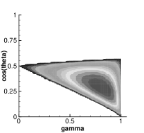
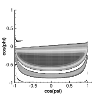
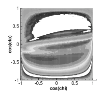
Figure 2: Left most figure: Initial condition parameter plane for ${\mathbf{u}}^{(1)}$. For $\gamma=0$, the Kelvin wave is periodic in time; for values of $\gamma,\cos\theta$ which fall into the white region for $\gamma>0$, the Kelvin wave is quasiperiodic, that is, the periods of ${\mathbf{a}}^{(1)}$ and ${\mathbf{k}}^{(1)}$ are rationally related; for the remaining region, the Kelvin wave has an exponentially growing amplitude. Center figure: Initial orientation parameter plane for ${\mathbf{u}}^{(2)}$ at ${\mathbf{x}}={\mathbf{0}}$ with parameter values $\cos\theta=0.2$, $\gamma=0$ and $\mu^{(1)}\beta^{(1)}=1$. For parameter values which fall into the white regions, the amplitude of ${\mathbf{a}}^{(2)}$ is bounded; for all others, the amplitude of ${\mathbf{a}}^{(2)}$ grows exponentially in time. Right figure: Initial orientation parameter plane for ${\mathbf{u}}^{(3)}$ at ${\mathbf{x}}={\mathbf{0}}$ with parameter values $\cos\theta=0.2$, $\gamma=0$, $\cos\phi=0.5$, $\cos\psi=0$. For parameter values which fall into the white regions, the amplitude of ${\mathbf{a}}^{(3)}$ is bounded; for all others, the amplitude of ${\mathbf{a}}^{(3)}$ grows exponentially in time.

4.2 Secondary instability

We now construct the next WKB-bootstrap iteration as ${\mathbf{u}}^{(2)}={\mathcal{S}}{\mathbf{x}}+\mu^{(1)}{\mathbf{a}}^{(1)}\sin(\beta^{(1)}\Phi^{(1)})+\mu^{(2)}{\mathbf{a}}^{(2)}\sin(\beta^{(2)}\Phi^{(2)})$. The equations for the phase $\Phi^{(2)}$ and the amplitude ${\mathbf{a}}^{(2)}$ are given in Eqs. (9)-(12) with ${\mathbf{U}}={\mathbf{u}}^{(1)}$. In the interest of simplicity, we consider the case $\cos\theta=0.2,\gamma=0$. Then ${\mathbf{u}}^{(1)}$ is periodic with period $2\pi$, and the equation for ${\mathbf{a}}^{(2)}$ again satisfies a Floquet problem. We further simplify our analysis by examining the flow at the origin, which is a fixed point of the system. Then, $\Phi^{(1)}=0$ and ${\mathcal{L}}^{(2)}={\mathcal{S}}+\mu^{(1)}\beta^{(1)}{\mathbf{a}}^{(1)}({\mathbf{k}}^{(1)})^{T}$. Note that although $\Phi^{(1)}=0$ and $\Phi^{(2)}=0$ at this fixed point, this does not imply that the phases are commensurate. Indeed, we choose the initial condition for the wave vector ${\mathbf{k}}^{(2)}$ to be arbitrary in three-dimensions: ${\mathbf{k}}^{(2)}(0)=[\cos\psi\sin\phi,\sin\psi\sin\phi,\cos\phi]^{T}$. The center figure in Fig. 2 shows the domain in the $(\cos\phi,\cos\psi)$ plane for which the amplitude of ${\mathbf{a}}^{(2)}$ grows exponentially. This figure first appeared in Lifschitz & Fabijonas (1996) in which the authors examined the stability of Bayly’s solution for $\gamma=0$ using GOSM. We conclude, then that the analysis of Lifschitz & Fabijonas (1996) is also an exact solution of the full nonlinear Euler equations. This result applies to the subsequent articles by the same authors and their collaborators Fabijonas et al. (1997); Fabijonas & Lifschitz (1998). The authors viewed the perturbation analysis of ${\mathbf{u}}^{(1)}$ as a secondary perturbation analysis of ${\mathbf{u}}^{(0)}$.

4.3 Tertiary instability

We construct a third iteration of this method as ${\mathbf{u}}^{(3)}={\mathcal{S}}{\mathbf{x}}+\mu^{(1)}{\mathbf{a}}^{(1)}\sin(\beta^{(1)}\Phi^{(1)})+\mu^{(2)}{\mathbf{a}}^{(2)}\sin(\beta^{(2)}\Phi^{(2)})+\mu^{(3)}{\mathbf{a}}^{(3)}\sin(\beta^{(3)}\Phi^{(3)})$, where the phases are incommensurate. Again, we examine the case $\cos\theta=0.2$, $\gamma=0$ at the fixed point ${\mathbf{x}}={\mathbf{0}}$, and additionally we choose $\cos\phi=0.5$ and $\cos\psi=0$. Thus, the flow ${\mathbf{u}}^{(2)}$ is bounded in time, and ${\mathcal{L}}^{(3)}={\mathcal{S}}+\mu^{(1)}\beta^{(1)}{\mathbf{a}}^{(1)}({\mathbf{k}}^{(1)})^{T}+\mu^{(2)}\beta^{(2)}{\mathbf{a}}^{(2)}({\mathbf{k}}^{(2)})^{T}$. The individual components of ${\mathbf{u}}^{(2)}$ are periodic, but there is no apparent common period. To analyze the evolution of ${\mathbf{a}}^{(3)}$, we use a quasi-periodic analogue of Floquet theory as discussed in detail in Bayly et al. (1996). We use the incompressibility condition ${{\mathbf{a}}^{(3)}}\cdot{{\mathbf{k}}^{(3)}}=0$ to reduce Eq. (10) for ${\mathbf{a}}^{(3)}$ to a two-dimensional system. We then use the Prüfer transformation

$$a_{1}^{(3)}(t)=e^{d(t)}\cos[c(t)],\quad a_{2}^{(3)}(t)=e^{d(t)}\sin[d(t)]\,,$$ (18)

where $a_{1}^{(3)}$ and $a_{2}^{(3)}$ are the first two components of ${\mathbf{a}}^{(3)}$. This produces a coupled pair of ordinary differential equations for $c(t)$ and $d(t)$. Note that linear growth of $d(t)$ implies exponential growth for ${\mathbf{a}}^{(3)}$. One can define two quantities called the growth rate $I$ and the winding number $W$ as

$$I=\lim_{t\to\infty}[d(t)/t],\quad W=\lim_{t\to\infty}[c(t)/t],$$ (19)

respectively. It was first shown conclusively in Bayly et al. (1996) that these quantities my be approximated by long time simulations independently of the values of $c(0)$ and $d(0)$. We choose the initial condition for ${\mathbf{k}}^{(3)}$ in polar coordinates as before: ${\mathbf{k}}^{(3)}(0)=[\cos\chi\sin\eta,\sin\chi\sin\eta,\cos\eta]^{T}$. The right figure in Fig. 2 shows the parameter plane $(\cos\eta,\cos\chi)$ for which the amplitude ${\mathbf{a}}^{(3)}$ grows exponentially in time for a specific orientation of ${\mathbf{a}}^{(2)}$. In the spirit of Lifschitz & Fabijonas (1996), we may view this as a tertiary perturbation of the rigidly rotating flow which again provides an exact nonlinear NS solution.

5 Discussion

The present analysis extends the previous results for stability of a rigidly rotating column of fluid with circular streamlines. Bayly (1986) showed that though this case was stable in the presence of a traveling wave, slight perturbations in the streamline eccentricity yield a traveling wave whose amplitude grows exponentially in time (left figure in Fig. 2). Furthermore, Lifschitz & Fabijonas (1996) showed that while the primary traveling wave was always stable, the amplitude of a secondary wave with an incommensurate phase grows exponentially (center figure in Fig. 2). In the present paper, we show that even when the secondary wave is stable (that is, then the amplitude is bounded for all time), the tertiary wave is unstable for a larger portion of its parameter space. Thus, we conclude that a circular columnar flow is critically stable in the sense that either perturbations in the eccentricity or the addition of incommensurate phases will result in waves whose amplitudes grow exponentially in time.

This paper has accomplished three main objectives. First, we extended the pioneering work of Craik & Criminale (1986) and Bayly (1986) to allow nonlinear instability analysis of any exact solution of the NS equations due to multi-harmonic Kelvin waves, evaluated along a flowline in the Lagrangian frame of the base flow. Second, we showed how to construct a sequence of exact solutions to the NS equations that involves the multi-frequency superposition of Kelvin traveling waves by adding the waves one at a time. This iterative method of constructing exact NS solutions was called ‘WKB-bootstrapping.’ Third, we used the WKB-bootstrapping method to unite and extend various classical linearized instability analyses of a circular columnar flow.