Control of chaotic transport in Hamiltonian systems

Abstract

It is shown that a relevant control of Hamiltonian chaos is possible through suitable small perturbations whose form can be explicitly computed. In particular, it is possible to control (reduce) the chaotic diffusion in the phase space of a Hamiltonian system with $1.5$ degrees of freedom which models the diffusion of charged test particles in a “turbulent” electric field across the confining magnetic field in controlled thermonuclear fusion devices. Though still far from practical applications, this result suggests that some strategy to control turbulent transport in magnetized plasmas, in particular tokamaks, is conceivable.

Transport induced by chaotic motion is now a standard framework to analyze the properties of numerous systems. Since chaos can be harmful in several contexts, during the last decade or so, much attention has been paid to the so-called topic of chaos control. Here the meaning of control is that one aims at reducing or suppressing chaos inducing a relevant change in the transport properties, by means of a small perturbation (either open-loop or closed-loop control of dissipative systems limapet ; review ) so that the original structure of the system under investigation is substantially kept unaltered. Control of chaotic transport properties still remains an open issue with considerable applications.
In the case of dissipative systems, an efficient strategy of control works by stabilizing unstable periodic orbits, where the dynamics is eventually attracted. Hamiltonian description of microscopic dynamics usually involves a large number of particles. However, methods based on targeting and locking to islands of regular motions in a “chaotic sea” are of no practical use in control when dealing simultaneously with a large number of unknown trajectories. Therefore, the only hope seems to look for small perturbations, if any, making the system integrable or closer to integrable. In what follows we show that it is actually possible to control Hamiltonian chaos by preserving the Hamiltonian structure.
Chaotic transport of particles advected by a turbulent electric field with a strong magnetic field is associated with Hamiltonian dynamical systems under the ${\bf E\times B}$ guiding center approximation nota . Although it has been shown that the $\bf E\times B$ drift motion of the so-called guiding center can lead to a diffusive transport in a fairly good agreement with the experimental counterparts marc88 ; marctur , it is clear that such an analysis is only a first step in the investigation and understanding of turbulent plasma transport. The control of transport in magnetically confined plasmas is of major importance in the long way to achieve controlled thermonuclear fusion. Two major mechanisms have been proposed for such a turbulent transport, transport governed by the fluctuations of the magnetic field and transport governed by fluctuations of the electric field. There is presently a large consensus to consider, at low plasma pressure, that the latter mechanism agrees with experimental evidence Scott . In the area of transport of trace impurities, i.e. that are sufficiently diluted so as not to modify the electric field pattern, the present model should be the exact transport model. Even for this very restricted case, control of chaotic transport would be very relevant for the thermonuclear fusion program. The possibility of reducing and even suppressing chaos combined with the empirically found states of improved confinement in tokamaks, suggest to investigate the possibility to devise a strategy of control of chaotic transport through some smart perturbation acting at the microscopic level of charged particle motions.
First, we briefly describe the Hamiltonian with $1.5$ degrees of freedom modeling the ${\bf E}\times{\bf B}$ motion of charged test particles in a “spatially turbulent” electric field. Then we formulate the problem of control and analytically derive the partial control term for a Hamiltonian describing the motion of these test particles. Finally, we report the numerical evidence of the effectiveness of the method. Let us begin by describing the model whose dynamics we want to control. In the guiding center approximation, the equations of motion of charged particles in the presence of a strong toroidal magnetic field and of a nonstationary electric field are

$${\dot{\bf x}}=\frac{d}{dt}{x\choose y}=\frac{c}{B^{2}}{\bf E}({\bf x},t)\times{\bf B}=\frac{c}{B}{-\partial_{y}V(x,y,t)\choose\partial_{x}V(x,y,t)},$$ (1)

where $V$ is the electric potential, ${\bf E}=-{\bf\nabla}V$, and ${\bf B}=B{\bf e_{z}}$. To define a model we choose

$$V({\bf x},t)=\sum_{\bf k}{V_{\bf k}}\sin[{\bf k}\cdot{\bf x}+\varphi_{\bf k}-\omega({\bf k})t],$$ (2)

where $\varphi_{\bf k}$ are random phases and the set of $V_{\bf k}$’s decreases as a given function of $|{\bf k}|$, in agreement with experimental data anormal_exp . In principle, one should use for $\omega({\bf k})$ the dispersion relation for electric drift waves (which are thought to be responsible for the observed turbulence) with a frequency broadening for each ${\bf k}$ in order to model the experimentally observed spectrum $S({\bf k},\omega)$. Unfortunately this would be prohibitive from a computational point of view, therefore one is led to simplify the model drastically by choosing $\omega({\bf k})=\omega_{0}$ constant and the phases $\varphi_{\bf k}$ at random to reproduce a turbulent field (with the reasonable hope that the properties of the realization thus obtained are not significantly different from their average). In addition we take for $|{V_{\bf k}}|$ a power law in $|{\bf k}|$ to reproduce the spatial spectral characteristics of the experimental $S({\bf k})$, see Ref. anormal_exp . Thus we consider the following explicit form for the electric potential

$$V(x,y,t)=\frac{a}{2\pi}\sum_{m,n=1\atop{n^{2}+m^{2}\leq N^{2}}}^{N}\frac{\sin\left[\frac{2\pi}{L}(nx+my)+\varphi_{nm}-\omega_{0}t\right]}{(n^{2}+m^{2})^{3/2}}~{}.$$ (3)

By rescaling space and time, we can always assume that $L=1$ and $\omega_{0}=1$. In what follows, we choose $N=25$. The spatial coordinates $x$ and $y$ play the role of the canonically conjugate variables. We extend the phase space $(x,y)$ into $(x,y,E,\tau)$ where the new dynamical variable $\tau$ evolves as $\tau(t)=t+\tau(0)$ and $E$ is its canonical conjugate. We absorb the constant $c/B$ of Eq. (1) in the amplitude $a$, so that we can assume that $a$ is small when $B$ is large. The autonomous Hamiltonian of the model is

$$H(x,y,E,\tau)=E+V(x,y,\tau)~{}.$$ (4)

The equations of motion are

$${\dot{x}}=\frac{\partial H}{\partial y}=\frac{\partial V}{\partial y}~{},\ \ \ \ \ \ \ {\dot{y}}=-\frac{\partial H}{\partial x}=-\frac{\partial V}{\partial x}~{},\ \ \ \ \ \ \ {\dot{\tau}}=1~{},$$ (5)

and $E$ is given by taking $H$ constant along the trajectories. Thus, for small values of $a$, Hamiltonian (4) is in the form $H=H_{0}+\epsilon V$, that is an integrable Hamiltonian $H_{0}$ (with action-angle variables) plus a small perturbation $\epsilon V$. For simplicity we assume that the average of $V$ over the angles is zero. Otherwise similar calculations following these lines can be done. The problem of control in Hamiltonian systems is to find a small perturbation term $f$ such that $H+f$ is integrable. In this article, we are interested in finding a partial control term $f_{2}$ of order $\epsilon^{2}$ such that the Hamiltonian given by $H_{c}=H_{0}+\epsilon V+\epsilon^{2}f_{2}$ is closer to integrability, i.e. such that $H_{c}$ is canonically conjugate to $H_{0}+O(\epsilon^{3})$. We perform a Lie transform on $H_{c}$, generated by a function $S$:

$$H^{\prime}_{c}=e^{\epsilon\hat{S}}H_{c}\equiv H_{c}+\epsilon\{S,H_{c}\}+\frac{\epsilon^{2}}{2}\{S,\{S,H_{c}\}\}+....,$$ (6)

where $\{\cdot~{},\cdot\}$ is the Poisson bracket and the operator $\hat{S}$ is acting on $H$ as $\hat{S}H=\{S,H\}$. An expansion in power series in $\epsilon$ of $H^{\prime}_{c}$ gives

$$H^{\prime}_{c} = H_{0}+\epsilon\left[\{S,H_{0}\}+V\right]$$

$$+\epsilon^{2}\left[f_{2}+\{S,V\}+\frac{1}{2}\{S,\{S,H_{0}\}\}\right]+O(\epsilon^{3})~{}.$$

The generating function $S$ is chosen such that

$$\{S,H_{0}\}+V=0~{},$$ (8)

provided that this equation has a solution. The control term $f_{2}$ given by the cancellation of order $\epsilon^{2}$ terms $[$and using Eq. (8)$]$,

$$f_{2}=-\frac{1}{2}\{S,V\},$$ (9)

satisfies the required condition that $H_{c}$ is canonically conjugate to $H_{0}$ up to order $\epsilon^{3}$ terms. We notice that by adding higher order terms in $\epsilon$ in the control term, one can build $f$ such that $H_{c}=H+\epsilon^{2}f$ is integrable for sufficiently small $\epsilon$ (see Ref. michel for more details and for a general formulation and theorem).
In the case we consider, $H_{0}=E$ and Eq. (8) becomes

$$-\frac{\partial S}{\partial t}+V=0~{},$$ (10)

and so $S$ is one primitive in time of $V$. We choose the one with zero time average. For the model (3), the generating function $S$ is

$$S(x,y,\tau)=\frac{a}{2\pi}\sum_{m,n=1\atop n^{2}+m^{2}\leq N^{2}}^{N}\frac{\cos\left[2\pi(nx+my)+\varphi_{nm}-\tau\right]}{(n^{2}+m^{2})^{3/2}}~{},$$ (11)

and the computation of $f_{2}$ gives

$$f_{2}(x,y,\tau)=\frac{a^{2}}{8\pi}\sum_{n_{1},m_{1},n_{2},m_{2}}\frac{n_{2}m_{1}-n_{1}m_{2}}{(n_{1}^{2}+m_{1}^{2})^{3/2}(n_{2}^{2}+m_{2}^{2})^{3/2}}$$

$$\times\sin\bigl{[}2\pi\bigl{[}(n_{1}-n_{2})x+(m_{1}-m_{2})y\bigr{]}+\varphi_{n_{1}m_{1}}-\varphi_{n_{2}m_{2}}\bigr{]}~{}.$$

We note that for the particular model (3), the partial control term $f_{2}$ is independent of time.
With the aid of numerical simulations (see Ref. marc88 for more details on the numerics), we check the effectiveness of the above control by comparing the diffusion properties of particle trajectories obtained from Hamiltonian (3) and from the same Hamiltonian with the control term (Control of chaotic transport in Hamiltonian systems). Figures 1 and 2 show the Poincaré surfaces of section of two trajectories issued from the same initial conditions computed without and with the control term respectively. Similar pictures are obtained for many other randomly chosen initial conditions. A clear evidence is found for a relevant reduction of the diffusion in presence of the control term (Control of chaotic transport in Hamiltonian systems).

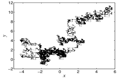
Figure 1: Poincaré surface of section of a trajectory obtained for Hamiltonian (3) assuming $a=0.8$.

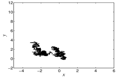
Figure 2: Poincaré surface of section of a trajectory obtained for the same initial condition as in Fig.1 and adding the control term (Control of chaotic transport in Hamiltonian systems) to Hamiltonian (3) .

In order to study the diffusion properties of the system, we have considered a set of $\mathcal{M}$ particles (of order $100$) uniformly distributed at random in the domain $0\leq x,y\leq 1$ at $t=0$. We have computed the mean square displacement $\langle r^{2}(t)\rangle$ as a function of time

$$\langle r^{2}(t)\rangle=\frac{1}{\mathcal{M}}\sum_{i=1}^{\mathcal{M}}{|{\bf x}_{i}(t)-{\bf x}_{i}(0)|}^{2}$$ (13)

where ${\bf x}_{i}(t),~{}i=1,\dots,\mathcal{M}$ is the position of the $i$-th particle at time $t$ obtained by integrating Eq. (5) with initial condition ${\bf x}_{i}(0)$. Figure 3 shows $\langle r^{2}(t)\rangle$ for three different values of $a$.

Figure 3: Mean square displacement $\langle r^{2}(t)\rangle$ versus time $t$ obtained for Hamiltonian (3) with three different values of $a=0.7,0.8,0.9$.

For the range of parameters we consider, the behavior of $\langle r^{2}(t)\rangle$ is always found to be linear in time for $t$ large enough. The corresponding diffusion coefficient is defined as

$$D=\lim_{t\rightarrow\infty}{{\langle r^{2}(t)\rangle}\over t}~{}.$$

Figure $4$ shows the values of $D$ as a function of $a$ with and without control term. It clearly shows a significant decrease of the diffusion coefficient when the control term is added. As expected, the action of the control term gets weaker as $a$ is increased towards the strongly chaotic phase.

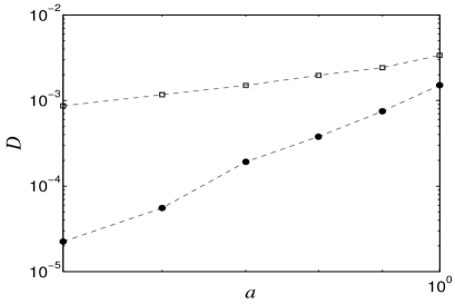
Figure 4: Diffusion coefficient $D$ versus $a$ in log-log scales obtained for Hamiltonian (3) (open squares) and Hamiltonian (3) plus control term (Control of chaotic transport in Hamiltonian systems) (full circles).

We check the robustness of the control by replacing $f_{2}$ by $\delta\cdot f_{2}$ and varying the parameter $\delta$ away from its reference value $\delta=1$. Figure 5 shows that increasing or decreasing $\delta$ from $\delta=1$ result in a loss of efficiency of the control. The fact that a larger perturbation term ($\delta>1$) does not work better than the one with $\delta=1$ means that the perturbation is “smart” and that it is not a “brute force” effect.

Figure 5: Diffusion coefficient $D$ versus $\delta$ magnitude of the control term (Control of chaotic transport in Hamiltonian systems) for a fixed value of $a=0.7$

Let us define the horizontal step size (resp. vertical step size) as the distance covered by the test particle between two successive sign reversals of the horizontal (resp. vertical) component of the drift velocity. The effect of the control is analyzed in terms of the Probability Distribution Function (PDF) of step sizes. Following test particle trajectories for a large number of initial conditions, with and without control, leads to the PDFs plotted in Fig. $6$. A marked reduction of the PDF is observed at large step sizes with control relatively to the not controlled case. Conversely, an increase is found for the smaller step sizes.

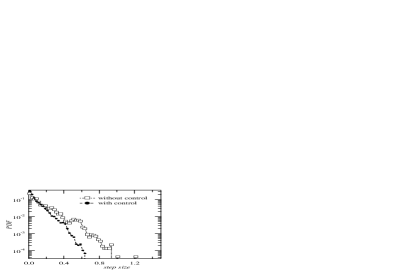
Figure 6: PDF of the magnitude of the horizontal step size with and without the control term.

The control quenches the large steps, typically larger than $0.5$.
In order to measure the relative magnitude between Hamiltonian (3) and $f_{2}$, we have numerically computed their mean squared values:

$$\sqrt{\frac{\langle f_{2}^{2}\rangle}{\langle V^{2}\rangle}}\approx 0.13a~{}~{},$$ (14)

which means that the control term can be considered a small perturbative term (when $a<1$).

So to conclude this work, we have provided an effective new strategy to control the chaotic diffusion in Hamiltonian dynamics using small perturbations. Since the formula of the control term is explicit, we are able to compare the dynamics without and with control in a simplified model, describing anomalous electric transport in magnetized plasmas. Even though we use a rather simplified model to describe chaotic transport of charged particles in fusion plasmas, our result makes conceivable that to apply some smart perturbation can lead to a relevant reduction of the turbulent losses of energy and particles in tokamaks.

References

- (1) e-mail: ciraolo@arcetri.astro.it
- (2) e-mail: chandre@cpt.univ-mrs.fr
- (3) e-mail: lima@cpt.univ-mrs.fr
- (4) e-mail: pettini@arcetri.astro.it
- (5) e-mail: vittot@cpt.univ-mrs.fr
- (6) e-mail: charles.figarella@cea.fr
- (7) e-mail: philippe.ghendrih@cea.fr
- (8) G. Chen and X. Dong, Int. J. Bif. & Chaos, 3, 1363 (1993).
- (9) R. Lima and M. Pettini, Phys. Rev. A 41, 726 (1990); Int. J. Bif. & Chaos 8, 1675 (1998); L. Fronzoni, M. Giocondo, M. Pettini, Phys. Rev. A 43, 6483 (1991).
- (10) Interestlingly enough, the dynamics of test particles streaming along a field line in a fusion device are also governed by Hamiltonian dynamics, the Hamiltonian being either the poloidal or toroidal magnetic flux. The principle of control of stochastic transport would apply equally well to magnetic turbulence.
- (11) M. Pettini et al., Phys. Rev. A 38, 344 (1988).
- (12) M. Pettini, “Low Dimensional Hamiltonian Models for Non-Collisional Diffusion of Charged Particles”, in Non-Linear Dynamics (Bologna, 1988), G. Turchetti, Ed. World Scientific (Singapore, 1989) 287.
- (13) B. D. Scott, Phys. Plasmas, 10, 963 (2003) and the list of references therein.
- (14) A.J. Wootton et al., Phys. Fluids B, 2, 2879 (1990).
- (15) M. Vittot: Perturbation Theory and Control in Classical or Quantum Mechanics by an Inversion Formula , archived in http://arxiv.org/pdf/math-ph/0303051