Recurrence Time Statistics for Finite Size Intervals

Abstract

We investigate the statistics of recurrences to finite size intervals for chaotic dynamical systems. We find that the typical distribution presents an exponential decay for almost all recurrence times except for a few short times affected by a kind of memory effect. We interpret this effect as being related to the unstable periodic orbits inside the interval. Although it is restricted to a few short times it changes the whole distribution of recurrences. We show that for systems with strong mixing properties the exponential decay converges to the Poissonian statistics when the width of the interval goes to zero. However, we alert that special attention to the size of the interval is required in order to guarantee that the short time memory effect is negligible when one is interested in numerically or experimentally calculated Poincaré recurrence time statistics.

The recurrence of trajectories to a neighborhood of a region in the phase space can be used to analyze important properties of dynamical systems. When this tool is applied to experimental or numerical generated data the limit of infinitely small recurrence interval(the Poincaré limit) is never achieved. In this article, we present a new effect that appears due to the finite size of the recurrence interval and changes the exponential decay of the distribution of recurrence times. The results are analyzed for the logistic and Hénon maps but are expected to apply to a large class of chaotic dynamical systems.

 

I Introduction

Since it was settled, the Poincaré recurrence theorem has been the source of a number of paradoxes relating reversible microscopic dynamics of a system on the one hand and irreversible macroscopic behavior of this system on the other hand. An answer to these paradoxes was given by Boltzmann, who adopted the law of big numbers ($N\rightarrow\infty$, where $N$ is the number of degrees of freedom of the system under study) and the recognition that the Poincaré Recurrence Time (PRT) to a highly improbable initial condition is too large to be observed in times normally available. Boltzmann’s point of view was recently restated by Lebowitz [1] in contrast with a new point of view based on nonlinear dynamics. In this new approach, rather than the limit $N\rightarrow\infty$, the central role is played by the sensitivity to initial conditions added to the idea that the Poincaré recurrence time do not need to be very large to lie beyond the observable range limit [2, 3].

Besides its fundamental importance for classical statistical mechanics [4, 5], PRT statistics has been used, in the recent years, as a tool for time series analysis in a variety of areas ranging from economics to plasma physics [6, 7, 8, 9], and as a way of studying trapping properties in Hamiltonian systems [10, 11, 12], which is an important feature for anomalous transport processes [13, 14]. The series of recurrence times itself has also been subject of fractal analysis [15, 16, 17]. All these aspects have brought a renewed interest in the study of recurrence time statistics.

General results have shown that the exponential-one law, $e^{-t}$, holds for the cumulative probability of first recurrence times (scaled by the mean first recurrence time) of transitive Markov chains [18], hyperbolic dynamical systems such as axiom A diffeomorphisms [19] and for systems verifying a strong mixing property [20]. Further improvement to the study of recurrences to finite size intervals has been given by Galves and Schmitt [21]. They have computed an upper bound for the difference between the cumulative probability of first recurrence times and the exponential-one law. Moreover, they have shown that the right scaling of the first recurrence times should include an extra factor besides the mean first recurrence time. This factor lies between two strictly positive constants independent of the recurrence interval. Recently these results have been extended to unimodal maps [22].

The Poissonian statistics, or its cumulative equivalent exponential-one law for scaled recurrence times, is deduced in the limit of infinitely small recurrence interval. However, in many of the recent applications mentioned previously the recurrence times are obtained either from numerical simulations or experimental data. In these cases it is unavoidable to use a recurrence interval with a finite size. The size of the interval is chosen in order to obtain a sufficient number of recurrences to build the recurrence time (RT) statistics. In this article we are interested in the RT statistics to finite size intervals of chaotic dynamical systems.

We begin using simple basic concepts of combinatorial analysis to deduce the statistics of recurrences to a given finite size interval for random processes and chaotic systems with strong mixing. This statistics applies not only for the first recurrence time (RT) but for all the $r$-th recurrence time. We obtain this statistics, which we call binomial-like distribution of RT, as a result of a simple combinatorial analysis problem. This distribution is valid for every size of the return region. When the probability of coming back to the return region is very small, the binomial-like RT statistics reduces to the Poissonian statistics, commonly observed for PRT problems in the literature [16, 9, 23]. Since we adopt a combinatorial approach to deduce this statistics, almost no information about the dynamics of the system, but its strong chaotic mixing property, can be obtained from it. Therefore, dynamical properties show their signature when the recurrence time statistics deviates from the former ones. One of these deviations is particularly important for Hamiltonian systems and concerns with a power law tail for long recurrence times [23]. In this article, we study a type of deviation which is related with the presence of unstable periodic orbits inside of the recurrence interval. We call it short time memory effect. This deviation originates the extra factor, which should multiply the mean recurrence time in order to give the right scaling of the series of recurrence times as considered by Galves and Schmitt [21]. It appears when a finite recurrence interval is considered. Although this deviation is restricted to a few short recurrence times, it changes the whole statistics. Moreover, we would like to emphasize that our deviation is in agreement with the bounds estimated in the previous works.

The article is structured as follows: in section II, we present the deduction of the binomial-like statistics, which is exemplified by a Gaussian stochastic process. The statistics for chaotic dynamical systems (logistic and Hénon map) are calculated numerically in section III, where the short time memory effect is clearly observed. In section IV, we explore the origins of this effect and how it changes the RT statistics. Finally, in section V, we summarize our conclusions of this article.

II Binomial-like Distribution

Let $f:M\rightarrow M$ be a homeomorphism with an invariant measure $\mu(M)=1$. Given a region $I\subset M$ with $\mu(I)>0$, the Poincaré Recurrence Theorem asserts that a trajectory, having started inside $I$, returns to $I$ infinitely many times. The time interval, $T_{i}$, between the $i$-th and the $(i+r)$-th return is what we refer to as the $r$-th recurrence time. This time interval is just one of an infinite sequence $\{T_{i}:i=1,2,\ldots,\infty\}$, and we are interested in the statistics of this sequence.

For convenience, most of the calculations are made for unidimensional systems. In this case, the interval $I$ is defined as $I(X_{c},\delta)=[X_{c}-\delta,X_{c}+\delta]$, as illustrated in FIG. 1 with a Gaussian random time series. When we have small values of $\delta$, and thus a small probability $\mu(I)$, we are dealing with the Poincaré recurrence time.

Figure 1: First recurrence time to the interval $I$ for a random time series with Gaussian distribution.

This article concerns the discrete time case, where the system is observed at a constant sample rate $\tau=1$. A few adjustments are needed for the continuous time case [24, 25].

In order to obtain the statistics for the recurrence time, consider the following simple problem: Let $e_{1}$ and $e_{2}$ be two mutually exclusive events. The event $e_{1}$ occurs with the constant probability $\mu$ and $e_{2}$ with the constant probability $(1-\mu)$. Consider now a sequence of $T_{i}$ trials $\{S_{k}:k=1,2,\ldots,T_{i}\}$ where $S_{k}=e_{1}$ or $S_{k}=e_{2}$. What is the probability of having $r$ events of type $e_{1}$ and $(T_{i}-r)$ events of type $e_{2}$ with the constraint that the last trial results is an event of the type $e_{1}$? This kind of problem is known in the literature of combinatorial analysis as Bernoulli trials (“repeated independent trials for which there are only two possible outcomes with probabilities that remain the same throughout the trials” [26]).

The answer for this problem is the following: the probability of having $r$ events $e_{1}$ and $(T_{i}-r)$ events $e_{2}$ is $\mu^{r}(1-\mu)^{T_{i}-r}$. The last event must be of the type $e_{1}$, then there are

$$\dfrac{(T_{i}-1)!}{(T_{i}-r)!(r-1)!}$$

ways of having $(r-1)$ events $e_{1}$ in the previous $(T_{i}-1)$ trials. Combining these results and suppressing the index $i$, since $T_{i}$ is just one of an infinite sequence of $r$-th recurrence times, we have:

$$P(T;r,\mu)=\dfrac{(T-1)!}{(T-r)!(r-1)!}\mu^{r}(1-\mu)^{T-r}\,.$$ (1)

For a dynamical system with an invariant ergodic measure and for which each step is independent from the previous ones, it is easy to see that Eq. (1) gives the probability of $r$-th recurrence time if we consider the following analogy: between the $i$-th and the $(i+r)$-th return to the interval $I(X_{c},\delta)$ the trajectory spends $T_{i}$ steps, each step (one trial) has a probability $\mu=\mu(I(X_{c},\delta))$ of being in the interval $I(X_{c},\delta)$ (event $e_{1}$) and a probability $[1-\mu(I(X_{c},\delta))]$ of being outside $I(X_{c},\delta)$ (event $e_{2}$).

Usually one is interested in the first recurrence time statistics ($r=1$). In this case, Eq. (1) gives

$$P(T;1,\mu)=\mu(1-\mu)^{T-1}\,,$$ (2)

that can be rewritten as

$$P(T;1,\mu)=\dfrac{\mu}{1-\mu}e^{\ln(1-\mu)T}\,,$$

which, by its turn, reduces to the Poissonian statistics

$$P(T;1,\mu)=\mu e^{-\mu T}\,,$$ (3)

when $\mu\rightarrow 0$.

This statistics is the one commonly encountered for Poincaré recurrences in chaotic dynamical systems [6, 16]. The small $\mu(I(X_{c},\delta))$ condition is, usually, satisfied when we take small values of $\delta$.

For any $r$, in the usual limit [26], $\mu\rightarrow 0$ and $T\gg 1$, the binomial-like distribution (Eq. (1)) reduces to the Poisson-like distribution

$$P(T;r,\mu)=\dfrac{\mu(\mu T)^{r-1}}{(r-1)!}e^{-\mu T}\,.$$ (4)

Eqs. (2) and (3), as well as any other distribution of first RT, must satisfy two conditions: the first one is, obviously, the normalization,

$$\sum_{T=1}^{\infty}P(T;1,\mu)=1\,,$$ (5)

and the second one is the Kac’s lemma [24, 5, 27]:

$$\langle T\rangle\equiv\sum_{T=1}^{\infty}T\,P(T;1,\mu)=\dfrac{\tau}{\mu}\,.$$ (6)

Although Kac’s lemma is usually applied to closed Hamiltonian systems, its original derivation [24] was based in general assumptions that cover a large class of dynamical systems including those we shall discuss in this work.

The above conditions will be used in section IV to take into account dynamical effects on the recurrence time statistics.

To finalize this section we shall exemplify the binomial-like distribution obtaining the RT statistics of a stochastic process whose variable, $x$, is governed by a Gaussian density of probability:

$$\rho_{G}(x)=\dfrac{1}{\sqrt{2\pi\sigma^{2}}}e^{-\dfrac{(x-\langle x\rangle)^{2}}{2\sigma^{2}}}\,,$$ (7)

with $\langle x\rangle=0$ and $\sigma=0.2$ (see FIG. 2).

Figure 2: Gaussian density of probability with $\langle x\rangle=0$ and $\sigma=0.2$. The probabilities of returning to the regions $I_{1}$ and $I_{2}$ is given by $\mu_{1}$ and $\mu_{2}$, respectively.

The probability, $\mu(I(X_{c},\delta))$, of returning to an interval $I(X_{c},\delta)$ is given by:

$$\mu(I(X_{c},\delta))=\int_{X_{c}-\delta}^{X_{c}+\delta}\rho_{G}(x)dx\,,$$ (8)

in particular, for the intervals $I_{1}$ and $I_{2}$, shown in FIG. 2, we have $(X_{c1}=0.3,\delta_{1}=0.02)$ and $(X_{c2}=-0.2,\delta_{1}=0.06)$, respectively. Their corresponding probabilities are $\mu(I_{1})=0.02596$ and $\mu(I_{2})=0.09679$.

FIG. 3 shows the statistics of recurrences to the intervals $I_{1}$ and $I_{2}$ for the Gaussian random time series.

Figure 3: The $r$-th RT statistics for a Gaussian random walk. We chose arbitrary values of $r$ and the two intervals illustrated in FIG. 2. The solid lines are given by Eq. (1).

The solid lines correspond to the analytical results given by Eq. (1) and they are in a good agreement with the numerical results.

III Chaotic dynamical systems

Let’s see now what happens when we consider the statistics of first recurrence of two deterministic dynamical systems.

The first system we analyze is the logistic map,

$$x_{n+1}=b\,x_{n}(1-x_{n})\,,$$ (9)

in the completely chaotic regime (parameter $b=4$). Its invariant probability density,

$$\rho_{L}(x)=\dfrac{1}{\pi\sqrt{x(1-x)}}\,,$$ (10)

is shown in FIG. 4. In this figure, we also see the return interval $I_{1}$ ($X_{c1}=0.9,\delta_{1}=0.01$) with measure $\mu(I_{1})=0.02124$.

Figure 4: Invariant probability density for the logistic map. The marked area, $\mu_{1}$, represents the measure of the interval $I_{1}(X_{c1}=0.9,\delta_{1}=0.01)$.

Using the logistic map, we create a trajectory with $N=10^{8}$ points and look for recurrences to the interval $I_{1}=[X_{c1}=0.9,\delta_{1}=0.01]$, indicated in FIG. 4. The statistics of first recurrence times to this interval is shown in FIG. 5.

Figure 5: Recurrence time distribution for a logistic map ($I_{1}=[X_{c}=0.9,\delta=0.01]$ and $N=10^{8}$ points) trajectory. The dashed line is the binomial-like distribution for $\mu(I_{1})=0.02124$ (which coincides with the corresponding Poissonian distribution). The full line is the curve calculated to satisfy (5) and (6) after $T=n^{*}=10$. The inset is an amplification of the small return times region and the squares are the analytic calculation of the return time probability as explained in FIG. 7.

As our second example of dynamical system we choose the Hénon map,

$$\begin{split}x_{n+1}&=1-a\,x_{n}^{2}-y_{n}\,,\\ y_{n+1}&=b\,x_{n}\,.\end{split}$$ (11)

with the parameters $a=1.4$ and $b=0.3$.

Figure 6: Recurrence time statistics for the Hénon map with $I(\mathbf{X}_{c},\delta)$ given by $\mathbf{X}_{c}=(0.304,0.210)$ and $\delta=10^{-2}$. The total of $10^{7}$ recurrence events were considered. Dashed line is the binomial-like distribution for $\mu(I)=\langle T\rangle^{-1}=0.00785$. The inset is an amplification of the short recurrence times region.

The distribution of first recurrence to a finite size interval for the Hénon map is shown in FIG. 6. In order to obtain this result, we eliminate the transient by iterating the Hénon map $10^{3}$ times and take the final point, $\mathbf{X}_{c}=(x_{c},y_{c})$, as the center of the phase space interval, $I$, with radius $\delta=10^{-2}$. An initial condition inside the interval $I$ is chosen and the Hénon map is iterated until we obtain $10^{7}$ recurrence events.

Both maps present distributions of recurrence times which fall exponentially (a straight line for a linear-log graphic) after some $T\geq n^{*}$ ($n^{*}\approx 10$ for the logistic map and $n^{*}\approx 40$ for the Hénon map). What is indicated through the solid lines in FIG. 5 and FIG. 6 for the logistic map and Hénon map, respectively. Nevertheless, these solid lines do not coincide with the ones (dashed lines) given by the binomial-like statistics, Eq. (2), which is indistinguishable from what would be the correct Poissonian statistics with $\langle T\rangle=\dfrac{1}{\mu(I)}$ for the particular size of the intervals used. In particular, the difference between the right mean recurrence time and the inverse of the slope of the solid line in figure 6 is approximately $9.3\%$. This difference indicates that an extra factor, besides the mean recurrence time, should be considered in order to obtain the right scaling of the series of recurrence times [21].

The reason for this deviation is the following: In the previous section, we showed that the complete independence of iteration and the existence of an invariant measure were necessary to obtain the binomial-like statistics of recurrence to an interval of finite size. However, deterministic dynamical systems hardly fulfill the condition that an iteration is completely independent from the previous ones. Therefore, dynamical systems have a kind of memory which affects the distribution of short recurrence times as we shall show in the next section.

IV Memory Effects on the RT Distribution

In this section, we show how the memory effect changes the probability of short recurrence times, and how the latests are responsible for the deviation of the whole distribution.

We take the advantage of working with a simple dynamical system, the logistic map, which gives us the possibility of calculating analytically the probability of short recurrence times.

IV.1 Short Recurrences and Lack of Memory

The procedure to obtain the probability of short recurrence times, illustrated in FIG. 7, consists in identifying the region, $R_{n}\subset I$, of initial points whose trajectories return to $I$ after $n$ iterations of the map $f(x)$, what is equivalent to the first recurrence of the map $f^{n}(x)$.

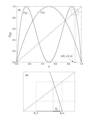
Figure 7: Analytic calculation for the return time probability for $T=2$ in the logistic map. The region $R_{2}$ represents the points inside $I$ that return to $I$ after two iterations of the map. We also see that $R_{1}=\varnothing$.

Since we are specially interested in the first return time, we note that, if $R_{n}\cap R_{m}\neq\varnothing$ for $m<n$, the points from the intersection will return to $I$ in $m$, not $n$, iterations. To avoid this error, we define a new interval $\bar{R}_{n}=R_{n}-(R_{n}\cap R_{m})$ for every $m<n$. The probability of a first recurrence time $T=n$ is, then, given by:

$$P_{1}(T=n)=\dfrac{\mu(\bar{R}_{n})}{\mu(I)}\,.$$ (12)

This method provides the probability of any first recurrence time. Nevertheless, the determination of the regions $\bar{R}_{n}$ becomes a cumbersome task as $n$ grows.

Although the above procedure is not useful for calculating the probabilities of first return when $n$ becomes large, it is useful for showing how the chaotic dynamics simulates a random process for large recurrence times.

When $n$ grows, the region $R_{n}$ becomes the union of a large number, $N$, of disjoint sub-regions in the interval $I$, that is:

$$R_{n}=\bigcup_{i=1}^{N}R^{i}_{n}\,,\quad\text{with}\quad\mu(R_{n})=\sum_{i=1}^{N}\mu(R^{i}_{n})\,.$$ (13)

The more sub-regions we have, the smaller they are.

In particular, as the map $f^{n}(x)$ is a polynomial of order $2^{n}$ there are $2^{n}$ unstable periodic orbits, each one with its associated sub-region. The $2^{n}$ sub-regions are distributed in the interval $[0,1]$ according to the invariant density, $\rho_{L}(x)$, given by Eq. (10). The sub-regions $R^{i}_{n}$ are just the ones which are inside the interval $I$.

For large $n$, there are $N\approx 2^{n}\mu(I)$ sub-regions in the interval $I$, each one with the same measure,

$$\mu(R^{i}_{n})=\dfrac{\mu(I)}{2^{n}}\,.$$ (14)

The probability of having a recurrence to $I$ in the time $T=n$ is:

$$P(T=n)=\dfrac{\mu(R_{n})}{\mu(I)}\,.$$ (15)

Putting Eqs. (13) and (14) in Eq. (15), we obtain the recurrence probability, $P(T=n)\approx\mu(I)$, independent of $n$ for large $n$, which is the same hypothesis assumed for the Bernoulli trials problem in section II. This argument justifies the exponential decay of the recurrence time statistics after the short times. It must be emphasized, however, that $P(T)$ given by Eq. (15) is not the probability of first recurrence to $I$ in the time $T=n$. This one is given by Eq. (12), where $\bar{R}_{n}$, instead of $R_{n}$, is used. It is in the calculations of $\bar{R}_{n}$ that the memory effect appears, since the approximation $N\approx 2^{n}\mu(I)$ is not valid for $n<n^{*}$. The same arguments hold for a general hyperbolic chaotic system, since the number of recurrence sub-regions is equal to the number of periodic orbits, and the latest grows as $e^{hT}$, where $h$ is the topological entropy.

IV.2 The Fitting of the Memoryless Exponential

Let’s see how the deviation of the shortest recurrence times affects the whole distribution. As it was shown in FIG. 5, for greater values of $T$ (after the decay of the memory, $T>n^{*}$) the recurrence time distribution approaches a straight line in a linear-log graphics, what can be generally represented by an exponential,

$$P_{exp}(T)=g_{0}e^{-\gamma T}.$$ (16)

Since we know the mean recurrence time (or the measure of the recurrence interval), the above two parameters, $g_{0}$ and $\gamma$, can be analytically obtained by using the two conditions presented in section II, namely, the normalization:

$$\sum_{T=1}^{n^{*}-1}P_{1}(T)+\sum_{T=n^{*}}^{\infty}P_{exp}(T)=1\,,$$ (17)

and the Kac’s lemma:

$$\langle T\rangle=\sum_{T=1}^{n^{*}-1}TP_{1}(T)+\sum_{T=n^{*}}^{\infty}TP_{exp}(T)=\dfrac{1}{\mu(I)}\,,$$ (18)

where $P_{1}(T)$ is given by Eq. (12) or obtained directly from the data. The agreement of the exponential (Eq. (16)) obtained by this procedure with the linear part (in the linear-log representation) of the RT distribution for the logistic map, as shown by the solid lines in FIG. 5 and FIG. 6, was verified for different recurrence intervals.

IV.3 Dependence of the memory effect on the interval

In this sub-section, we explore the dependence of the memory effect on the position $X_{c}$ and size of the interval with a special interest in small intervals. As we argued before, only a few number of short recurrence times diverge from a straight line in the linear-log representation, but their effects on the whole distribution is considerable. So we can take the deviation of the asymptotic exponential from the binomial (Poissonian) distribution as a quantifier of the short time memory effect. Let

$$g(T)=g_{0}e^{-\gamma T}\,,$$

be the exponential adjusted to the asymptotic part of the distribution. As shown in section II, the binomial distribution results in $\gamma=-ln(1-\mu)$, that reduces to $\gamma=\mu$ in the Poissonian case. Since we are specially interested in small intervals, we will use the relative deviation from the Poisson statistics $\gamma/\mu(I)-1=\gamma\langle T\rangle-1$ as the quantifier of the memory effect.

In FIG. 8, it is shown the dependence of the memory effect with the position of the interval. We note that the effect occurs for virtually all recurrence intervals. Most of the intervals deviate from the exponential positively but for recurrence intervals that contain periodic orbits of small periods the asymptotic exponential is negatively deviated when compared to the binomial distribution.

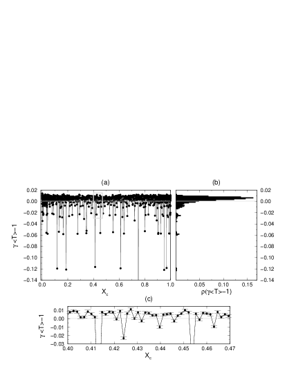
Figure 8: Dependence of the memory effect $(\gamma\langle T\rangle-1)$ on the position of the recurrence interval $(X_{c})$. (a) Results for the $10^{3}$ intervals with measure $\mu(I)=10^{-3}$, centered in $X_{c}$, that covers the interval $x\in[0,1]$ of the logistic map. (b) histogram of (a). (c) amplification of (a) showing the size of the fitting errors. The gray line represents the expected value for the binomial distribution.

To explore the dependence of the memory effect on the size of the interval we took, by chance, an arbitrary position $X_{c}=0.582$ and we vary its semi-width, $\delta$. The results obtained numerically are illustrated in FIG. 9. For the logistic map, the relation between the measure, $\mu(I)$, and the semi-width, $\delta$, is easily found out integrating the distribution (10)

$$\begin{split}\mu(X_{c},\delta)&=\int_{X_{c}-\delta}^{X_{c}+\delta}\dfrac{1}{\pi\sqrt{(x(1-x))}}\,dx\\ &=\arcsin(X_{c}+\delta)-\arcsin(X_{c}-\delta)\,.\end{split}$$ (19)

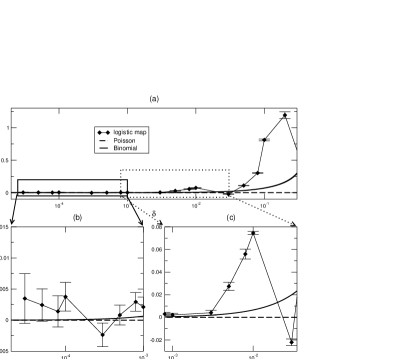
Figure 9: Dependence of the memory effect $(\gamma\langle T\rangle-1)$ on the size of the recurrence interval $(\delta)$. The position of the interval was chosen randomly as $X_{c}=0.582$. The dashed and solid lines are the expected results for the Poisson and binomial distribution respectively. (b) and (c) are amplifications of (a) for small values of $\delta$ and show the convergence to the binomial statistics for $\delta<10^{-4}$ in the fitting precision.

With the relation (19) and remembering that for the binomial distribution $\gamma=-ln(1-\mu)$ we obtain the solid line in FIG. 9. From FIG. 9, we see that for great values of $\delta$ the results deviate from both the Poissonian (dashed line) and binomial-like distributions. The convergence of the numerical results of the logistic map to the Poissonian statistics occurs in the limit of small interval, coherently with what is found in the literature [22]. This convergence occurs clearly only for $\delta<10^{-4}$. Considering the error bars obtained by the numerical fitting, these are much smaller intervals than the ones for which the convergence of the binomial-like to Poisson takes place. Considering our previous discussions, the convergence of the numerical results to the Poissonian statistics occurs only when the short time memory effect becomes negligible.

V Conclusions

Based on a simple Bernoulli trials problem, we obtain a binomial-like distribution for the $r$-th recurrence time statistics of a generic interval. This distribution depends only on the measure of the recurrence interval ($\mu(I)$) that, when it is sufficiently small, turns out the statistic to the usual Poissonian distribution for the first Poincaré recurrence time.

The information related to the dynamical properties appears in the deviation from these distributions as, for example, the power-law behavior for large recurrence times studied in references [10, 13]. In this article, we discuss a kind of deviation that appears for finite size intervals. In this case the short recurrence times are affected by a kind of memory of the chaotic systems. We show that the origin of this short time memory effect is due to the existence of unstable periodic orbits inside of the finite size recurrence interval. The analytical method of calculating the recurrence probabilities, described in section IV.1, shows how these periodic orbits changes the distribution of short recurrence times. Furthermore, our observed deviations for the specific systems studied in this work are in agreement with bounds predicted for general classes of systems in previous works [18, 19, 20, 21].

The exponential growth of the number of periodic unstable orbits in chaotic dynamical systems restates the condition of independence between recurrences for large times, resulting in an exponential-like behavior of the recurrence time distribution after the decay of memory. Imposing the normalization condition and the Kac’s lemma, we are able to make an analytical fitting to the memoryless part of the distribution. This fitting illustrates how the short recurrence times, which are affected by the memory, modify the whole distribution. Since just a few points deviate from an exponential, a histogram bin larger than one may lead to the wrong conclusion that the distribution is Poissonian. What results in a contradiction: the inverse of the false Poissonian exponent is different from the mean recurrence time obtained from the recurrence series. For example, for the data of FIG. 6 this difference is of $9.3\%$. We believe that this alert has to be taken into account when the RT statistics is calculated. We would like to stress that our results indicate that the correct normalization of a series of recurrence times should consider an extra factor, besides the mean recurrence time, in order to properly obtain the asymptotic exponential-one law.

We emphasize that the memory effect, discussed in this article, applies for any recurrence interval of a general chaotic dynamical system. For small intervals it may not be relevant because it turns smaller than the numeric precision. When one is calculating RT numerically, it must be checked that the interval is sufficiently small that this regime is already achieved.

- [1] J. L. Lebowitz. Reviews of Modern Physics, 71(2):346, 1999.
- [2] G. Aquino, P. Grigolini and N. Scafetta. Chaos, Solitons and Fractals, 12(11):2023, 2001.
- [3] D. Ruelle. Physica A, 263:540, 1999.
- [4] H. L. Frisch. Physical Review, 104(1):1, 1956.
- [5] M. Kac. Probability and Related Topics in Physical Sciences. Interscience, New York, 1959.
- [6] J. B. Gao. Physical Review Letters, 83(16):3178, 1999.
- [7] M. S. Baptista and I. L. Caldas. Physica A, 312:539, 2002.
- [8] M. S. Baptista, I. L. Caldas, M.V.A.P. Heller and A.A. Ferreira. Physics of Plasmas, 8(10):4455, 2001.
- [9] M. S. Baptista, I. L. Caldas, M.V.A.P. Heller, A.A. Ferreira, R. Bengtson and J. St ckel. Physica A, 301:150, 2001.
- [10] B. V. Chirikov. Physica D, 13:395, 1984.
- [11] J. D. Meiss. Chaos, 7(1):139, 1997.
- [12] H. Hu, A. Rampioni, L. Rossi and G. Turchetti. Chaos, 14(1):160, 2004.
- [13] G. M. Zaslavsky and M. K. Tippett. Physical Review Letters, 67(23):3251, 1991.
- [14] G. M. Zaslavsky, M. Edelman and B. A. Niyazov. Chaos, 7(1):159, 1997.
- [15] V. Afraimovich. Chaos, 7(1):12, 1997.
- [16] V. Afraimovich and G. M. Zaslavsky. Physical Review E, 55(5):5418, 1997.
- [17] N. Hadyn, J. Luevano, G. Mantica and S. Vaienti. Physical Review Letters, 88(22):224502, 2002.
- [18] B. Pitskel. Ergodic Theory Dynamical Systems, 11(3):501, 1991.
- [19] M. Hirata. Ergodic Theory Dynamical Systems, 13(3):533, 1993.
- [20] M. Hirata. Poisson law for the dynamical systems with the “self-mixing” conditions, volume Vol. 1. World Sci. Publishing, River Edge, NJ, 1995.
- [21] A. Galves and B. Schmitt. Random Comput. Dynam., 5(4):337, 1997.
- [22] H. Bruin and S. Vaienti. Fundamenta Mathematicae, 176:77, 2003.
- [23] G. M. Zaslavsky. Physics Reports, 371:461, 2002.
- [24] M. Kac. Bulletin of the American Mathematical Society, (53):1002, 1947.
- [25] V. Balakrishnan, G. Nicolis and C. Nicolis. Physical Review E, 61(3):2490, 2000.
- [26] W. Feller. An Introduction to probability theory and its applications. John Willey & Sons, New York, 1950.
- [27] I.P. Cornfeld, S.V. Fomin and Ya. G. Sinai. Ergodic Theory. Springer-Verlag, Berlin, 1982.