Formation of a Standing-Light Pulse through Collision of Gap Solitons

Abstract

Results of a systematic theoretical study of collisions between moving solitons in a fiber grating are presented. Various outcomes of the collision are identified, the most interesting one being merger of the solitons into a single zero-velocity pulse, which suggests a way to create pulses of “standing light”. The merger occurs with the solitons whose energy takes values between $0.15$ and $0.35$ of the limit value, while their velocity is limited by $\approx 0.2$ of the limit light velocity in the fiber. If the energy is larger, another noteworthy outcome is acceleration of the solitons as a result of the collision. In the case of mutual passage of the solitons, inelasticity of the collision is quantified by the energy-loss share. Past the soliton’s stability limit, the collision results in strong deformation and subsequent destruction of the solitons. Simulations of multiple collisions of two solitons in a fiber-loop configuration are performed too. In this case, the maximum velocity admitting the merger increases to $\approx 0.4$ of the limit velocity. Influence of an attractive local defect on the collision is also studied, with a conclusion that the defect does not alter the overall picture, although it traps a small-amplitude pulse. Related effects in single-soliton dynamics are considered too, such as transformation of an input sech signal into a gap soliton (which is quantified by the share of lost energy), and the rate of decay of a quiescent gap soliton in a finite fiber grating, due to energy leakage through loose edges.

I Introduction

Bragg gratings (BGs) are structures in the form of a periodic variation of the core refractive index, which are written on a fiber or other optical waveguide Kashyap . Devices based on fiber gratings, such as filters and gain equalizers, are among the most widely used components of optical systems. Gap solitons (in a more general context, they are called BG solitons Sterke ) exist in fiber gratings due to the interplay between the BG-induced effective dispersion and Kerr nonlinearity of the fiber material. Exact analytical solution for BG solitons in a standard model were found in Refs. Aceves ; Demetri , and their stability was studied later, showing that, approximately, half of them are stable (see details below) Tasgal ; stability . Spatial solitons and their stability in a model of planar BG-equipped waveguide, taking into regard two polarizations of light, were recently considered in Ref. Skryabin .

Lately, a lot of attention has been attracted to possibilities of capturing “slow light” slowlight , and, in particular, of slowly moving optical solitons slowsoliton in various settings. Fiber gratings are natural candidates for a nonlinear medium where it is potentially possible to stop the light, as zero-velocities BG solitons, in which the left- and right-traveling waves are in permanent dynamical equilibrium, are available as exact solutions Aceves ; Demetri , and a part of them are stable Tasgal ; stability . Actually, BG solitons that were thus far observed in the experiment were fast ones, moving at a velocity $\approx 75\%$ of the limit light velocity in the fiber experiment . A possible way to create a zero-velocity soliton is to use an attractive finite-size Weinstein or $\delta$-like we local defect in the BG which attracts solitons (it was demonstrated in Ref. trapping that a defect can also stimulate a nonlinear four-wave interaction without formation of a soliton). Moreover, it is possible to combine the attractive defect with local gain, which opens a way to create a permanently existing pinned soliton, even in the presence of loss we2 .

One of objectives of this paper is to explore a possibility of slowing down BG solitons by colliding two identical ones moving in opposite directions in the fiber grating. Collisions are quite feasible from the experimental standpoint, as a characteristic length necessary for the formation of a BG soliton is $\simeq 2$ cm experiment , while uniform fiber gratings with a length $1$ m or even longer are now available. Already in the first work Aceves , where exact solutions for the moving solitons were found, their collisions were simulated, with a conclusion that they passed through each other, re-appearing with intrinsic vibrations, which may be explained by excitation of an intrinsic mode which a stable BG soliton supports Tasgal . Note that broad small-amplitude BG solitons are asymptotically equivalent to nonlinear-Schrödinger (NLS) solitons, hence collisions between them are completely elastic Litchinitser . However, in a more generic case results may be different, as the standard fiber-grating model, see Eqs. (1) below, is not an integrable one, on the contrary to the NLS equation. Systematic simulations are thus needed to study head-on collisions between BG solitons, results of which are reported below in Section III, after presenting the model in Section II. The main finding is that, at relatively small values of the solitons’s velocities $\pm c$, and not too large values of the solitons’ energy, the solitons merge into a single standing one. In the case when the solitons pass through each other, we quantify the collision by an energy-loss share. In section IV, we report results of simulations of multiple collisions between two solitons, to model a situation in a fiber loop. These results show that multiple collisions essentially increase the maximum velocity which admits the merger. Simulations were also carried out to check if inclusion of a local defect attracting the solitons may assist the fusion of the colliding solitons. In Section V we demonstrate that the defect does not affect the situation essentially; however, a small-amplitude trapped pulse, which captures a relatively small share of the initial solitons’ energy, appears as a result of the collision. Finally, in Section VI we report some related results pertaining to single-soliton dynamics, viz., reshaping of an input pulse of a sech form (as suggested by the NLS equation) into a BG soliton in the fiber grating, and gradual decay of a soliton in a finite-length grating due to the energy leakage through open ends. Section VII concludes the paper.

II The model

The commonly adopted model of nonlinear fiber gratings is based on a system of coupled equations for the right- ($u$) and left- ($v$) traveling waves Sterke ,

$$iu_{t}+iu_{x}+v+\left[\left(1/2\right)|u|^{2}+|v|^{2}\right]u = 0,$$

$$iv_{t}-iv_{x}+u+\left[\left(1/2\right)|v|^{2}+|u|^{2}\right]v = 0,$$ (1)

where $x$ and $t$ are the coordinate and time, which are scaled so that the linear group velocity of light is $1$, the Bragg-reflectivity coefficient being $1$ too. Exact solutions to Eqs. (1), which describe solitons moving at a velocity $c$ ($c^{2}<1$), were found in Refs. Aceves and Demetri :

$$u = \alpha W(X)\mathrm{exp}\,\left[y/2+i\phi(X)-iT\cos\theta+i\phi_{0}\right],$$

$$v = -\alpha W^{\ast}(X)\mathrm{exp}\,\left[-y/2+i\phi(X)-iT\cos\theta+i\phi_{0}\right].$$ (2)

Here, $\theta$ is an intrinsic parameter of the soliton family (the other parameter is $c$), which takes values $0<\theta<\pi$ and is proportional to the soliton’s energy (alias norm),

$$E\equiv\int_{-\infty}^{+\infty}\left[|u(x)|^{2}+|v(x)|^{2}\right]dx=8\theta\sqrt{1+c^{2}}\left(3+c^{2}\right)^{-1}.$$ (3)

Further, $\alpha^{-2}\equiv\frac{3}{2}+c^{2}$, $\tanh y\equiv c$, $\phi_{0}$ is an arbitrary real constant, and

$$X = \left(1-c^{2}\right)^{-1/2}\left(x-c\,t\right),\,T=\left(1-c^{2}\right)^{-1/2}\left(t-c\,x\right),$$

$$\phi(X) = \alpha^{2}\sinh(2y)\mathrm{\tan}^{-1}\left\{\tanh\left[(\sin\,\theta)X\right]\tan\left(\theta/2\right)\right\},$$ (4)

$$W(X) = \left(\sin\,\theta\right)\,\mathrm{sech}\left[(\sin\,\theta)X-i\left(\theta/2\right)\right]\,.$$

We used these exact solutions as initial conditions to simulate collisions between identical solitons with opposite velocities.

To consider the influence of a local defect on the collision (see Section V below), Eqs. (1) are modified as in Refs. Weinstein and we : To consider the influence of a local defect on the collision, Eqs. (1) are modified as in Refs. Weinstein and we :

$$iu_{t}+iu_{x}+v+\left[\left(1/2\right)|u|^{2}+|v|^{2}\right]u = -\delta(x)\left(\Gamma u-\kappa v\right),$$ (5)

$$iv_{t}-iv_{x}+u+\left[\left(1/2\right)|v|^{2}+|u|^{2}\right]v = -\delta(x)\left(\Gamma v-\kappa u\right),$$ (6)

where $\Gamma>0$ and $\kappa>0$ account for a local increase of the refractive index and suppression of the Bragg reflectivity, respectively.

III Collisions between solitons

III.1 The mode of simulations

In this section, we consider collisions between exact BG solitons (2). In a real experiment, an initially launched pulse should pass some distance to shape itself into a soliton. As it was mentioned above, in previously reported experiments this distance was quite small, $\sim 2$ cm experiment , hence this is not a big issue. Nevertheless, it is relevant to separately simulate shaping of an initially launched single-component pulse into a steady-shape BG soliton. This will be done separately below in section VI.

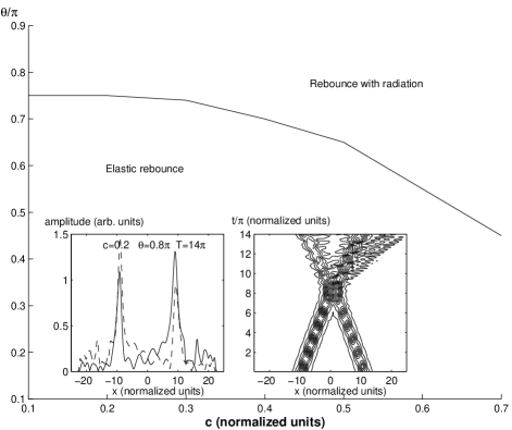
Figure 1: The border separating regions in the plane ($c,\theta_{\mathrm{in}}$) where, in the case of repulsion, the collision is elastic, or generates significant radiation loss. An example of the collision of the latter type is given in the inset, in which the left and right panels show, respectively, the waveforms $|u(x)|$ and $|v(x)|$ (solid and dashed lines) at the end of the simulation ($t=14\pi$), and the evolution of the field $|u(x,t)|$ in terms of level contours. Intrinsic “oscillations” of the solitons before the collision in the inset is an artifact due to mismatch between plotting sampling and the numerical grid used for the simulations.

Simulations of collisions were performed by means of the split-step fast-Fourier-transform method. First, collisions between solitons in the case of repulsion between them (with a phase difference $\Delta\phi_{0}=\pi$) was considered. It was found that the solitons bounce from each other quasi-elastically, without generation of any visible radiation or intrinsic vibrations of the solitons, if their initial velocities $\pm c$ are small enough, and the solitons are “light”, having a sufficiently small value of $\theta$. Collision-induced radiation becomes quite conspicuous if the solitons are “heavier” or faster, see an example in the inset to Fig. 1. Figure 1 shows a boundary in the plane $\left(c,\theta\right)$, above which the collision results in generation of noticeable amount of radiation, in the case $\Delta\phi_{0}=\pi$.

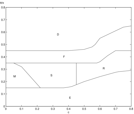
Figure 2: A diagram in the plane ($c,\theta_{\mathrm{in}}$) for different outcomes of the collision between in-phase solitons. In the region E the collision is elastic. In the region M, the solitons merge into a single pulse. In the region S, they separate with velocities smaller than they had before the collision. In the region R, the velocities are not affected by the collision, but conspicuous radiation losses are observed. In the region F, large radiation loss takes place, and the velocities increase after the collision. In the region D, the collision leads to strong deformation of the solitons.

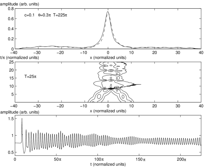
Figure 3: Typical examples of the collision between in-phase solitons. (a) Merger of the solitons in the region M in Fig. 3. They collide several times before the merger, which is accompanied by emission of radiation. The lower panel exhibits persistent vibrations of the field amplitude $|u(x=0,t)|$. Here and below, the middle and upper panels show, respectively, the evolution at a relatively early stage ($t=25\pi$), and the single pulse emerging at $t=225\pi$.

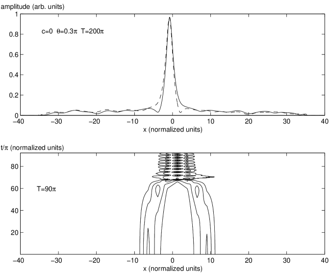
Figure 3: (b) Merger of initially quiescent solitons ($c=0$). The lower and upper panels show the evolution at $t<90\pi$, and the emerging single pulse at $t=200\pi$.

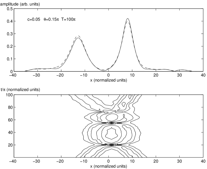
Figure 3: (c) At the lower edge of region M (Fig. 3), solitons undergo multiple collisions before they finally separate. Spontaneous symmetry breaking is evident in the final state.

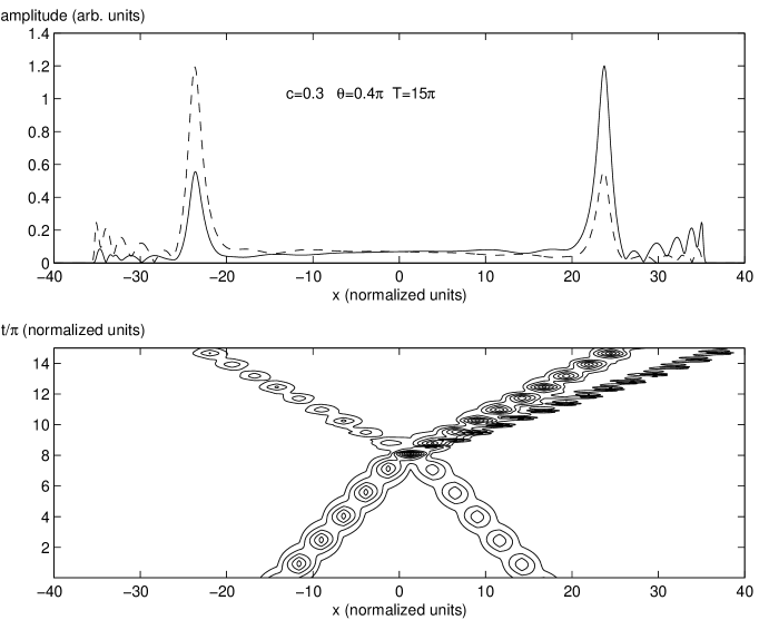
Figure 3: (d) Collision between relatively heavy solitons leads to emission of radiation jets and increase of the velocities (region F in Fig. 3).

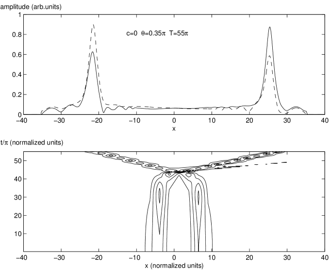
Figure 3: (e) Interaction between two initially quiescent solitons in the region F (Fig. 2).

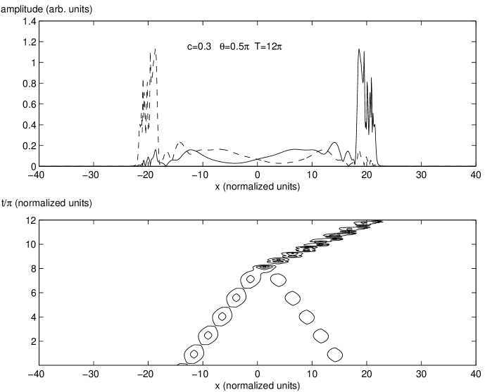
Figure 3: (f) Collision between heavy solitons which are weakly stable or unstable (region D in Fig. 2) results in strong deformation of the pulses, which is followed by their destruction (not shown here).

Then, collisions between in-phase solitons, with $\Delta\phi_{0}=0$ (the case of attraction), were simulated. In this case, a number of various outcomes can be distinguished. A summary of the results is displayed in Fig. 2 in the form of a diagram in the $(c,\theta)$ plane, different outcomes being illustrated by a set of generic examples displayed in Fig. 3.

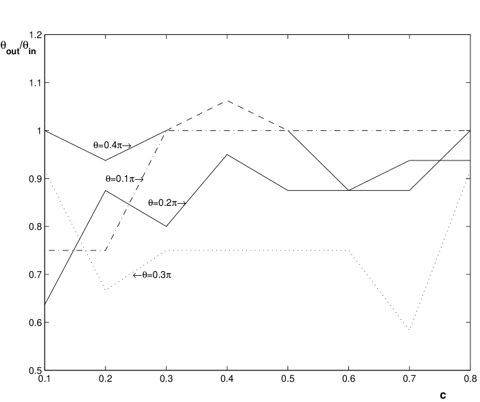
Figure 4: (a) The ratio of the post-collision soliton’s parameter $\theta_{\mathrm{out}}$, found from the least-square-error fit of the emerging pulse to the analytical waveforms (2), to the initial value $\theta_{\mathrm{in}}$. In this and next panels, the ratio is shown vs. the initial velocity $c$ at different fixed values of $\theta_{\mathrm{in}}$. The portion of the line corresponding to $\theta_{\mathrm{in}}=0.4\pi$ with $\theta_{\mathrm{out}}/\theta_{\mathrm{in}}>1$, which formally contradicts the energy conservation, is explained by the fact that in this case the actual shape of the emerging pulse is not very close to the analytical one, being more narrow.

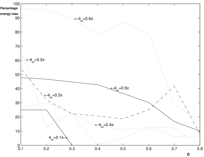
Figure 4: (b) The relative energy loss due to the collision of two solitons.

The simplest case is the collision of solitons with small $\theta$ (region E in Fig. 2; see also Fig. 4 below). In accordance with results reported in Ref. Litchinitser , these solitons collide elastically, which is easily explained by the fact that they are virtually tantamount to NLS solitons.

III.2 Merger of solitons and spontaneous symmetry breaking

The most interesting outcome of the collision is merger of two solitons into a single one, which takes place in the region $0\leq c<0.2$, $0.15\pi<\theta<0.35\pi$ (area M in Fig. 2). A typical example of the merger is shown in Fig. 3(a), its noticeable peculiarities being that the merger takes place after multiple collisions, and the finally established soliton demonstrates persistent internal vibrations, see the lower panel of Fig. 3(a). As judged from the lowest panel of Fig. 3(a) [and other similar plots], the amplitudes of these internal vibrations amount to about $10$ to $20\%$ of the soliton amplitudes. In this region (area M) of the values of $\theta$, the attraction between initially quiescent ($c=0$) in-phase solitons, which are placed at some distance from each other, also results in their merger, see Fig. 3(b). At the border between the regions M and E, the interaction between initially quiescent or slow solitons results in their separation after several collisions, which is accompanied by a conspicuous spontaneous symmetry breaking (SSB), see an example in Fig. 3(c). Note that the SSB resembles what was observed in a model of a dual-core fiber grating, in which the nonlinearity and BG proper were carried by different cores Atai . As well as in that case, SSB may be plausibly explained by a fact that the “lump”, which temporarily forms as a result of the attraction between the solitons in the course of the collision between them, may be subject to modulational instability, hence a small asymmetry in the numerical noise may provoke conspicuous symmetry breaking in the eventual state. Indeed, it is well known that any spatially uniform solution to Eqs. (1) is modulationally unstable MI , and it is obvious that the instability can extend to any sufficiently broad state.

III.3 Quasi-elastic collisions

Increase of $\theta$ brings one from the region M to F (Fig. 2), where solitons collide quasi-elastically, i.e., they separate after the collision, emerging with smaller amplitudes, see Fig. 3(d). A noticeable peculiarity of this case is that the collision results in an increase of the solitons’ velocities, which is seen in the change of the slope of the contour-level plots in Fig. 3(d). We note that, pursuant to Eq. (3), the soliton’s energy monotonically increases with $c^{2}$, therefore the collision-induced decrease of the amplitude may be explained not only by radiation loss, but also by the increase of the velocities. The acceleration of the solitons due to the collision is more salient if the initial velocity $c$ is small; for instance, initially quiescent solitons (with $c=0$) acquire a large velocity after the interaction, see Fig. 3(e).

As for still heavier solitons, it is known that they are unstable if $\theta>\theta_{\mathrm{cr}}\approx 1.011\cdot(\pi/2)$ Tasgal ; stability (this value pertains to $c=0$; $\theta_{\mathrm{cr}}$ very weakly depends on the soliton’s velocity stability ). In accordance with this, in the region D (Fig. 2) the collision triggers a strong deformation of unstable or weakly stable solitons, see Fig. 3(f). At essentially longer times, the strong deformation leads to destruction of the pulses.

If $\theta$ is taken in the same range as in the merger region M, i.e., $0.15\pi<\theta<0.35\pi$, but with a larger velocity, the collision picture seems in an ordinary way: the solitons separate with some decrease in their velocity, and some loss in the amplitude. If the initial velocity is still larger, it is possible to distinguish another region, marked R in Fig. 2, where the velocity shows no visible change after the collision, but emission of radiation takes place.

Quasi-elastic collisions can be naturally quantified by the ratio $\theta_{\mathrm{out}}/\theta_{\mathrm{in}}$ of the soliton’s parameter after and before the collision, and by share of the net initial energy of the solitons which is lost (to radiation) as the result of the collision. To this end, we performed the least-square-error fit of pulses emerging after the collision to the exact soliton solutions (2), aiming to identify the values of $\theta_{\mathrm{out}}$, and the post-collision velocity was measured in a straightforward way. The corresponding soliton’s energy was then calculated by means of the formula (3).

The results of the computation are shown in Fig. 4. A noteworthy feature, which is obvious in both panels (a) and (b), is that inelastic effects first strengthen with the increase of $\theta_{\mathrm{in}}$ from very small values (which correspond, as it was said above, to the NLS limit) to $\simeq 0.3\pi$, then they weaken, attaining a minimum, which corresponds to the most quasi-elastic collisions, at $\theta_{\mathrm{in}}\approx 0.4\pi$, and then get stronger again, with the increase of $\theta_{\mathrm{in}}$ up to $\simeq 0.6\pi$. Past the latter value, the isolated soliton is strongly unstable by itself, therefore detailed study of collisions becomes irrelevant.

IV Multiple collisions in a fiber ring

Since the main motivation of this work is the possibility to generate a standing pulse by dint of collisions between BG solitons, it is natural to consider multiple collisions, that may occur between two solitons traveling in opposite directions in a fiber loop, or if a single soliton performs shuttle motion in a fiber-grating cavity, i.e., a piece of the fiber confined by mirrors (in the latter case, the soliton periodically collides with its own mirror images). An issue for experimental realization of these schemes is to couple a soliton into the loop or cavity. Using a linear coupler connecting the system to an external fiber may be problematic, as repeated passage of the circulating soliton through the same coupler will give rise to conspicuous loss. Another solution may be to add some intrinsic gain to the system, making it similar to fiber-loop soliton lasers, where a soliton-circulation regime may self-start laser . It is relevant to mention that fiber-ring soliton lasers including BG components were investigated before BraggLaser . Still another possibility is to use figure-eight fiber lasers 8 , in which one loop is made of BG, while the other one provides for the gain. Detailed analysis of these schemes is, however, beyond the scope of this paper.

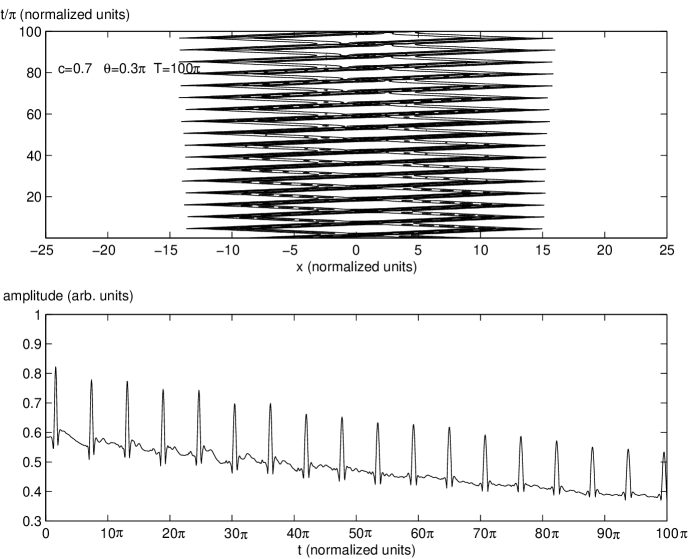
Figure 5: (b) Multiple collisions between solitons with the initial value $\theta=0.3\pi$ and initial velocities $\pm 0.7$ in the loop configuration.

We performed simulations of the multiple collisions between two identical solitons in the loop, imposing periodic boundary conditions. Figure 5(a) shows an example in which the multiple collisions slow down the solitons quite efficiently, enforcing them to merge. As is seen, in this case the solitons underwent two collisions before the merger. The initial values $c=0.3$ and $\theta=0.3\pi$ used in this example show that the multiple collisions in the loop help to increase the maximum initial velocity $c_{\max}$, that admits merger of the two solitons, by a factor of $3$ (at least) against the single-collision case, cf. Fig. 2. In fact, the largest value of $c_{\max}$ corresponding to the multiple collisions was found to be $\approx 0.4$, i.e., a part of the region S from Fig. 2 is absorbed into M in the loop configuration. The evolution of the field at the central point, $|u(x=0)|$, which is also displayed in Fig. 5(a), demonstrates that the emerging zero-velocity pulse is again a breather, cf. Fig. 3(a).

Another example of multiple collisions in the loop is shown in Fig. 5(b), where the solitons initially have $\theta=0.3\pi$ and $c=0.7$, belonging to the region R of Fig. 2. In this case, the solitons hardly undergo any slowing down due to the collisions, while they keep losing energy. Due to the gradual decrease of $\theta$, which is related to the energy by Eq. (3), the solitons gradually drift to the region E (see Fig. 2), where the collision becomes elastic.

V Effect of a localized defect on the collision.

In Refs. Weinstein and we , it has been found that local attractive defects can trap gap solitons. This fact suggests a possibility that the merger of two colliding solitons might be assisted by a defect placed at the collision point. We investigated the effect of two kinds of local defects, which represent BG suppression or increase of the refractive index, corresponding, respectively, to $\kappa>0$ and $\Gamma>0$ in Eqs. (6) (a single collision was considered in this case).

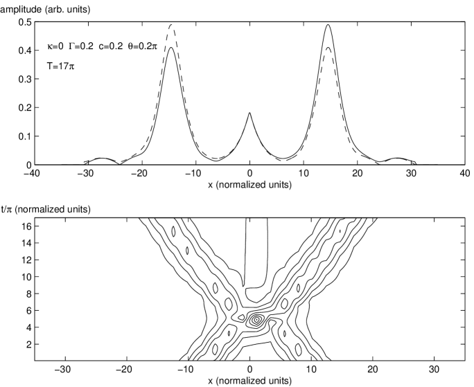
Figure 6: The collision between solitons with $\theta=0.2\pi$ and velocities $c=\pm 0.2$ in the case when a local perturbation of the refractive index, with $\Gamma=0.2$ [see Eqs. 6)], is placed at the collision point. The defect traps a small-amplitude soliton.

We have found that attractive defects of either type do not actually catalyze formation of a pinned pulse that would retain a large part of the energy of the colliding solitons. Nevertheless, a relatively small part of the energy gets trapped by the defect, and a small-amplitude pinned soliton appears, see an example in Fig. 6, which is displayed for the case of the local refractive-index perturbation, i.e., $\Gamma>0$, $\kappa=0$. Local BG suppression, accounted for by $\kappa>0$, produces a similar effect. We have also checked that repulsive local defects (negative $\Gamma$ or $\kappa$) do not produce any noticeable effect either.

VI Special effects in the single-soliton dynamics

VI.1 Transformation of an input pulse into a Bragg-grating soliton

As it was mentioned above, signals which are coupled into a fiber grating in a real experiment are not “ready-made” BG solitons, but rather pulses of a different form, which should shape themselves into solitons. After that, one can consider collisions between them, as it was done above. For this reason, it makes sense to specially consider self-trapping of BG solitons from a standard input pulse in the form of the NLS soliton,

$$u_{0}(x)=\eta\,\mathrm{sech}(\eta x)\exp(i\kappa x),\,v_{0}(x)=0.$$ (7)

where $\eta$ and $\kappa$ are two arbitrary real parameters. The energy of the pulse (7), defined as per Eq. (3), is $E_{0}=2\eta$.

Transformation of the pulse into a BG soliton was simulated directly within the framework of Eqs. (1). The results are summarized in Fig. 7, in the form of plots showing the share of the initial energy lost into radiation, cf. Fig. 4(b). A noteworthy feature revealed by the systematic simulations is that, with the increase of the parameter $\eta$, that measures the amplitude and inverse width of the initial pulse (7), the energy-loss share first decreases, attaining an absolute minimum at $\eta\simeq 0.8-1.0$, and then quickly increases. The fact that the relative energy loss becomes very large for large $\eta$ is easy to understand, as the initial energy of the pulse (7) increases indefinitely with $\eta$, while the energy of the emerging stable BG pulse, with $\theta\leq 1.011\cdot(\pi/2)$ and $c^{2}<1$, cannot exceed (in the present notation) $E_{\max}=\sqrt{2}\pi$, see Eq. (3) [we did not observe formation of more than one BG soliton from the initial pulse (7)]. Thus, an optimum shape of the sech input signal, which provides for the most efficient generation of the BG soliton, is suggested by these results.

VI.2 Decay of the soliton in a finite-length fiber grating with free ends

In any experiment (unless the fiber loop or cavity are used), a standing soliton will be created in a fiber grating with open edges. Then, some energy leakage will take place through free ends of the fiber segments. From the exact solution (2) it follows that the leakage is exponentially small if the segment’s length $l$ is much larger than the soliton’s spatial width, which is $\sim 1$ mm in a typical situation experiment ; we2 . Moreover, the energy leakage through loose end can be easily compensated (along with intrinsic fiber loss) by local gain we2 . Nevertheless, it is an issue of interest to find the soliton’s decay rate due to the leakage.

We addressed the issue, simulating Eqs. (1) with the free boundary conditions, $u_{x}=v_{x}=0$, set at the edges of the integration domain. In Fig. 8, we show the decay of the soliton’s amplitude in time, for different values of the domain’s length, with initial $\theta_{in}=0.51$. The initial increase of the amplitude is a result of temporary self-compression of the pulse due to its interaction with the edges. As a reference, we mention that, in the case of the shortest fiber grating considered here, with $l=8$, it takes the time $t=42.2$ for the decrease of the amplitude by a factor of $e$.

VII Conclusion

We have presented results of systematic studies of collisions between moving solitons in fiber gratings. Various outcomes of the collision were identified, the most interesting one being merger of the solitons into a single zero-velocity pulse, which suggests a way to create pulses of “standing light”. The merger occurs for solitons whose energy takes values between $0.15$ and $0.35$ of its maximum value, while the velocity is limited by $c_{\max}\approx 0.2$ of the limit velocity. If the energy is larger, another noteworthy outcome is acceleration of the solitons as a result of the collision, especially when their initial velocities are small. In the case when the solitons pass through each other, inelasticity of the collision was quantified by the relative energy loss. If the energy exceeds the soliton’s instability threshold, the collision results in strong deformation of the solitons, which is followed by their destruction. Simulations of multiple collisions between two solitons in the fiber-loop configuration show that the largest initial velocity admitting the merger increases to $c\leq c_{\max}\approx 0.4$ of the limit velocity. It was also shown that attractive local defects do not alter the overall picture, although a small-amplitude trapped pulse appears in this case. Finally, specific effects were investigated in one-soliton dynamics, such as transformation of a single-component pulse into a Bragg-grating soliton, and decay of the soliton in a finite-length fiber grating due to the energy leakage through loose edges.

Figures

Figure 5: (a) Multiple collisions between two solitons with the initial value $\theta=0.3\pi$, and initial velocity $\pm 0.3$ in the loop configuration. The upper and lower panels, respectively, show the global evolution of the field $|u(x,t)|$, and the evolution of its maximum. In the lower panel, the dotted parts of the curve mark two collisions (maximum overlappings) between the two solitons before they merge into a single pulse.

Figure 7: The relative energy loss in the process of self-trapping of the Bragg-grating soliton from the initial pulse (7) vs. the parameter $\kappa$ at fixed values of the amplitude $\eta$.

Figure 8: Decay of the field $|u(x,t)|$ at the central point of the finite fiber grating of length $l$ due to the energy loss through free ends.

References

- (1) R. Kashyap. Fiber Bragg gratings (Academic Press: San Diego, 1999).
- (2) C.M. de Sterke and J.E. Sipe, “Gap solitons”, Progr. Opt. 33, 203-260 (1994).
- (3) A.B. Aceves and S. Wabnitz, “Self-induced transparency solitons in nonlinear refractive periodic media”, Phys. Lett. A 141, 37-42 (1989).
- (4) D.N. Christodoulides and R.I. Joseph, Phys. Rev. Lett. 62, 1746 (1989).
- (5) B.A. Malomed and R.S. Tasgal, “Vibration modes of a gap soliton in a nonlinear optical medium”, Phys. Rev. E 49, 5787 (1994).
- (6) I.V. Barashenkov, D.E. Pelinovsky, and E.V. Zemlyanaya, “Vibrations and Oscillatory Instabilities of Gap Solitons”, Phys. Rev. Lett. 80, 5117-5120 (1998); A. De Rossi, C. Conti, and S. Trillo, Phys. Rev. Lett. 81, 85 (1998).
- (7) A.V. Yulin, D.V. Skryabin, and W.J. Firth, Phys. Rev. E 66, 046603 (2002).
- (8) J. Marangos, “Slow light in cool atoms”, Nature 397, 559-560 (1999); K.T. McDonald, “Slow light”, Am. J. Phys. 68, 293-294 (2000).
- (9) J.E. Heebner, R.W. Boyd, and Q.H. Park, “Slow light, induced dispersion, enhanced nonlinearity, and optical solitons in a resonator-array waveguide”, Phys. Rev. E 65, 036619 (2002).
- (10) B.J. Eggleton, R.E. Slusher, C.M. de Sterke, P.A. Krug, and J.E. Sipe, Phys. Rev. Lett. 76, 1627 (1996); C.M. de Sterke, B.J. Eggleton, and P.A. Krug, J. Lightwave Technol. 15, 1494 (1997).
- (11) R.H. Goodman, R.E. Slusher, and M.I. Weinstein,“Stopping light on a defect”, J. Opt. Soc. Am. B 19, 1635-1652 (2002).
- (12) W.C.K. Mak, B.A. Malomed, P.L. Chu,“Interaction of a soliton with a local defect in a fiber Bragg grating”, submitted to J. Opt. Soc. Am. B, in press.
- (13) C.M. de Sterke, E.N. Tsoy, and J.E. Sipe, “Light trapping in a fiber grating defect by four-wave mixing”, Opt. Lett. 27, 485-487 (2002).
- (14) W.C.K. Mak, B.A. Malomed, and P.L. Chu, Phys. Rev. E 67, 026608 (2003).
- (15) N.M. Litchinitser, B.J. Eggleton, C.M. de Sterke, A.B. Aceves, and G.P. Agrawal, “Interaction of Bragg solitons in fiber gratings”, J. Opt. Soc. Am. B 16, 18-23 (1999).
- (16) J. Atai and B.A. Malomed, Phys. Rev. E 64, 066617 (2001).
- (17) A.B. Aceves, C. De Angelis, and S. Wabnitz, Opt. Lett. 17, 1566 (1992).
- (18) L.E. Nelson, D.J. Jones, K. Tamura, H.A. Haus, and E.P. Ippen, Appl. Phys. B 65, 277 (1997).
- (19) P.K. Cheo, L. Wang, and M. Ding, IEEE Phot. Tech. Lett. 8, 66 (1996).
- (20) T.O. Tsun, M.K. Islam, and P.L. Chu, Opt. Commun. 141, 65 (1997).