A one-dimensional model of a dispersive medium with intrinsic loss, compensated by a parametric drive, is proposed. It is a combination of the well-known parametrically driven nonlinear Schrödinger (NLS) and complex cubic Ginzburg-Landau equations, and has various physical applications (in particular, to optical systems). For the case when the zero background is stable, we elaborate an analytical approximation for solitary-pulse (SP) states. The analytical results are found to be in good agreement with numerical findings. Unlike the driven NLS equation, in the present model SPs feature a nontrivial phase structure. Combining the analytical and numerical methods, we identify a stability region for the SP solutions in the model’s parameter space. Generally, the increase of the diffusion and nonlinear-loss parameters, which differ the present model from its driven-NLS counterpart, lead to shrinkage of the stability domain. At one border of the stability region, the SP is destabilized by the Hopf bifurcation, which converts it into a localized breather. Subsequent period doublings make internal vibrations of the breather chaotic. In the case when the zero background is unstable, hence SPs are irrelevant, we construct stationary periodic solutions, for which a very accurate analytical approximation is developed too. Stability of the periodic waves is tested by direct simulations.

1 Introduction

One of paradigm models adopted for the description of pulse dynamics in nonlinear dispersive media with intrinsic loss is the parametrically driven damped nonlinear Schrödinger (NLS) equation. In the one-dimensional case, it is

$$iu_{t}+\frac{1}{2}u_{xx}+\frac{1}{2}|u|^{2}u=(k-i)u+\gamma u^{\ast},$$ (1)

where $u(x,t)$ is the complex wave field, the asterisk stands for the complex conjugation, real $k$ is the frequency mismatch of the parametric drive, real $\gamma$ is the drive’s amplitude, which may be assumed positive, and the loss parameter, as well as the ones accounting for the spatial diffraction/dispersion and nonlinear frequency shift, are normalized to be $1$. Equation (1) finds applications to various physical problems, such as dynamics of spin waves in magnetics [1], plasma waves [2], and Faraday surface waves in a fluid layer driven by a time-periodic external force [3]. Arguably, the most realistic application of eq. (1) is to models of nonlinear optics, such as a cavity filled with a Kerr-nonlinear lossy material, the driving term being provided for by an external field supplied at the frequency coinciding with that of the signal field, see, e.g., ref. 4 and references therein.

It is well known that eq. (1) gives rise to two exact solutions for phase-locked solitons[5],

$$u(x)=A(x)e^{i\theta},\,A(x)=2\sqrt{k+\gamma\cos 2\theta}\,{\rm sech}\left(\sqrt{2(k+\gamma\cos 2\theta)}x\right),$$ (2)

where the phase constant takes values

$$\theta_{1}=-\frac{1}{2}\sin^{-1}\left(1/\gamma\right),\,\theta_{2}=\frac{1}{2}\left[\pi+\sin^{-1}\left(1/\gamma\right)\right]\,.$$ (3)

The solitons exist provided that $\gamma>1$.

The soliton with $\theta=\theta_{2}$, corresponding to the smaller value of the amplitude, $A_{0}\equiv 2\sqrt{k+\gamma\cos 2\theta}$, is always unstable, while the other one may be stable. The soliton stability in this model was studied in detail [6]. In particular, an obvious necessary condition is stability of the zero solution, which implies

$$k>\sqrt{\gamma^{2}-1}.$$ (4)

Thus, the stable soliton may exist in the interval $1<\gamma^{2}<1+k^{2}$ of the values of gain. Actually, the soliton is stable only in a part of this region, while in another part it is destabilized via a Hopf bifurcation, which was also studied in detail, see an earlier work [7] and a systematic analysis in refs. 8.

Another important dynamical model for pattern formation in nonlinear lossy media is based on the complex cubic Ginzburg-Landau (CCGL) equation, which may be written as

$$iu_{t}+(\beta_{1}-i\beta_{2})u_{xx}+(c_{1}+ic_{2})|u|^{2}u=(k+i)u,$$ (5)

where the coefficients $\beta_{1,2}$ and $c_{1,2}$ are real, and $\beta_{2}$ and $c_{2}$ cannot be negative. The linear-gain coefficient on the right-hand side of eq. (5) is normalized to be $1$ [cf. the normalized linear-loss coefficient in eq. (1)]. The CCGL equation has many applications, including description of the onset of turbulence in the Poiseuille flow [9] and Langmuir waves in plasmas [10]. Additionally, if $t$ and $x$ are replaced, respectively, by the propagation distance $z$ and reduced time $\tau$, eq. (5) describes the propagation of light signals in a pumped nonlinear optical waveguide, with the dispersion coefficient $\beta_{1}$, Kerr coefficient $c_{1}$, filtering coefficient $\beta_{2}$, and coefficient of two-photon absorption $c_{2}$ [11].

Various solutions to eq. (5) and their physical applications have been studied in detail, see a recent review [12]. A particular solution, which is unstable but nevertheless quite meaningful (see, e.g., a detailed consideration in ref. 13), is a solitary pulse (SP) that can be found in an exact analytical form [9, 10]

$$u=A\,_{0}\left[{\rm sech}\left(\kappa x\right)\right]^{1+i\mu}\exp\left(-i\omega t\right),$$ (6)

where all the real constants $A_{0},\kappa,\mu$ and $\omega\,$ are uniquely expressed in terms of parameters of eq. (5). It is noteworthy that the NLS equation proper, and its damped parametrically driven version (1), admit soliton solutions only under the condition which, in terms of eq. (5), is $\beta_{1}c_{1}>0$ (in terms of nonlinear optics, it implies that the nonlinear waveguide is either self-focusing with anomalous group-velocity dispersion, or self-defocusing with normal dispersion). However, except for the case $\beta_{2}=c_{2}=0$, the general CCGL equation (5) has the exact SP solution in the form (6) irrespective of the sign of the product $\beta_{1}c_{1}$, the only additional condition being that $\beta_{1}$ and $c_{1}$ must not simultaneously vanish. The most important difference of the SP solution (6) from the phase-locked soliton (2) is the presence of the chirp $\mu$, which accounts for a nontrivial intrinsic phase structure in the SP.

A natural generalization of both models (1) and (5) is a parametrically driven CCGL equation, which we take in the form

$$iu_{t}+(\beta_{1}-i\beta_{2})u_{xx}+(c_{1}+ic_{2})|u|^{2}u=(k-i)u+\gamma u^{\ast}.$$ (7)

It may apply to the above-mentioned physical systems under properly modified conditions. For instance, in the case of the nonlinear optical waveguide, eq. (7) describes a situation when the loss is compensated not by intrinsic gain, but rather by a co-propagating pump wave. It should be mentioned that a parametrically driven model of that type was already introduced in a two-dimensional situation, which corresponds to the light propagation in a planar nonlinear waveguide [14], and stable anisotropic two-dimensional SPs were found. In one dimension, a CCGL system with a nonlocal parametric drive was considered recently [15], but the straightforward one-dimensional model (7) has not been considered yet. Complex dynamics of interfaces was also studied using this type equation [16].

The existence of the stable soliton (2) in the driven-NLS limit of the model (7), and of the unstable SP (6) in its CCGL counterpart, suggest a possibility to find a SP solution to eq. (7) and investigate its stability, which is the subject of the present work. One may expect that an essential difference of the SP solution from its NLS phase-locked counterpart (2) is a nontrivial intrinsic phase structure (chirp).

In section 2, we report results obtained for SPs in the model (7). First, we develop an analytical approximation, that predicts all the properties of SPs, except for the chirp, with good accuracy. Then, we demonstrate numerical results, which are summarized in the form of stability diagrams in the model’s phase space. The stability domain shrinks with the increase of the diffusion and nonlinear-loss parameters $\beta_{1}$ and $c_{1}$ in eq. (7), which make it different from the NLS counterpart (1). At one of the domain’s borders, the soliton is destabilized via a Hopf bifurcation, which gives rise to a stable breather. The breathers are also briefly considered in section 2.

In the case when the condition (4) for the stability of the zero solution is not met, SPs keep to exist, but they cannot be stable. In this case, relevant solutions are periodic waves. We briefly consider them in section 3, also first in an approximate analytical form, and then by means of numerical methods. In this case, analytical and numerical results are virtually indistinguishable.

2 Solitary-pulses

2.1 Analytical approximation

To develop an analytical approximation to SP solutions, we fix two parameters in eq. (7), $\beta_{1}=c_{1}=1/2$, which can always be done by means of rescaling (provided that $\beta_{1}$ and $c_{1}$ are positive). We then assume an approximate form for the solution which mimics the exact solution (2) available in the NLS limit (1),

$$u(x)=A(x)e^{i\theta},$$ (8)

with constant $\theta$. Then, substituting the ansatz (8) into eq. (7), we formally obtain two different equations for the single real function $A(x)$:

$$\frac{d^{2}A}{dx^{2}}=2\left[k+\gamma\cos(2\theta)\right]A-A^{3},$$ (9)

$$\beta_{2}\frac{d^{2}A}{dx^{2}}=\left[1+\gamma\sin(2\theta)\right]A+c_{2}A^{3}.$$ (10)

We consider the case that $\beta_{2},\,1+\gamma\sin(2\theta)$ and $c_{2}$ are small. Eliminating the derivative term from eqs.(9) and (10), we arrive at a simpler relation,

$$(c_{2}+\beta_{2})A^{3}=\left(2\beta_{2}\left[k+\gamma\cos\left(2\theta\right)\right]-\left[1+\gamma\sin(2\theta)\right]\right)A.$$ (11)

An exact solution to eq. (9) is given by the expression for $A(x)$ from eq. (2), which we will use here, but without adopting the relation (3). Instead, we substitute the expression for $A(x)$ into eq. (11), then multiply all the equation again by $A(x)$, and integrate the result over $x$ from $-\infty$ to $+\infty$. This procedure leads to the following relation, that we use as a definition of $\theta$ in the waveform (2), which is now considered as an approximate solution to eq. (7):

$$2(k+\gamma\cos 2\theta)(4c_{2}+\beta_{2})+3\left[1+\gamma\sin\left(2\theta\right)\right]=0\,.$$ (12)

In particular, eq. (12), with regard to eq. (4), predicts that a stable SP solution may exist in the interval

$$\sqrt{\gamma^{2}-1}<k<k_{{\rm cr}}\equiv\frac{\gamma\sqrt{9+4(4c_{2}+\beta_{2})^{2}}-3}{2\left(4c_{2}+\beta_{2}\right)}\,.$$ (13)

With the increase of the combination $\left(4c_{2}+\beta_{2}\right)$, $k_{{\rm cr}}$ attains a minimum value,

$$\left(k_{{\rm cr}}\right)_{\min}=\sqrt{\gamma^{2}-1},$$ (14)

at

$$4c_{2}+\beta_{2}=\left(3/2\right)\sqrt{\gamma^{2}-1}$$ (15)

[at this point, the interval (13) collapses into a point]. With the further increase of $\left(4c_{2}+\beta_{2}\right)$, $k_{{\rm cr}}$ grows up to a maximum value, $\left(k_{{\rm cr}}\right)_{\max}\equiv k_{{\rm cr}}\left(4c_{2}+\beta_{2}=\infty\right)=\gamma.$

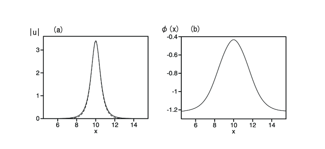
Figure 1: A typical example of the stable solitary pulse. The panels (a) and (b) show the amplitude and phase profiles of the stationary solution with $\gamma=1.5,k=2$ and $\beta_{2}=c_{2}=0.02$. In (a), the solid and dashed curves represent the numerical result and analytical approximation [based on Eqs. (2) and (12)], respectively.

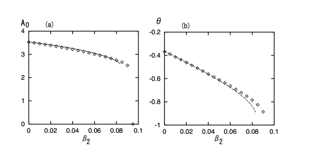
Figure 2: The amplitude of the solitary pulse (a) and its average phase (b), as defined in Eq. (16), vs. the parameter $\beta_{2}=c_{2}$. Other coefficients in Eq. (7) are fixed: $\gamma=1.5,k=2$. The symbols show numerical results, while continuous curves are predicted by the analytical approximation.

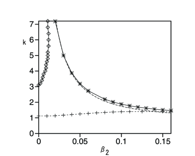
Figure 3: The region in the parametric plane with the coordinates $\beta_{2}=c_{2}$ and $k$ ($\gamma=1.5$ is fixed) in which stable solitary-pulse solutions were found. The curves connecting symbols which mark stability/existence borders are guides for the eye. The dashed curve, close to the upper right border, is the analytical prediction (13).

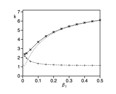
Figure 4: The solitary-pulse stability region in the parameter plane ($\beta_{1},k$) at fixed values $c_{1}=0.5,\beta_{2}=c_{2}=0.025$, and $\gamma=1.5$. The pulses are stable between the two borders. The dashed curve, close to the upper right border, is the analytical prediction.

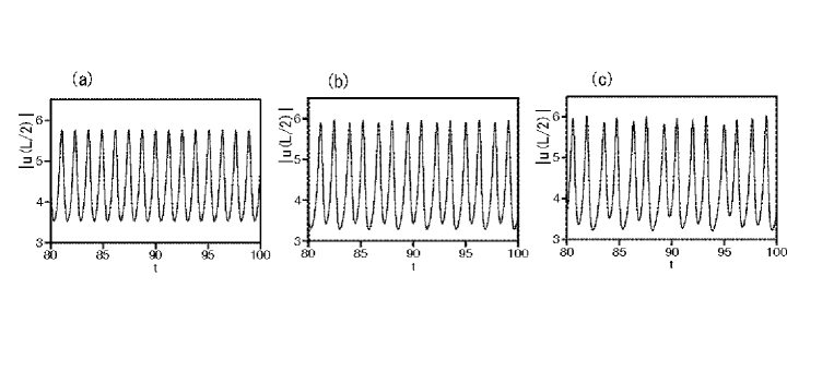
Figure 5: Time evolutions of the breather’s amplitude at (a) $\beta_{2}=c_{2}=0.005$, (b) $\beta_{2}=c_{2}=0.002$ and (c) $\beta_{2}=c_{2}=0.001$ in the case $k=4.5,c_{1}=\beta_{1}=0.5,\gamma=1.5$.

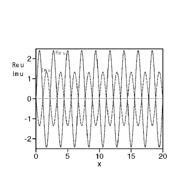
Figure 6: Comparison of the real and imaginary parts of the approximate analytical solution (17), i.e., $A_{0}{\rm cn}\left(\kappa x,q\right)\cos\theta$ (solid curve) and $A_{0}{\rm cn}\left(\kappa x,q\right)\sin\theta$ (dashed curve), and a direct numerical solution, in the case with $c_{2}=\beta_{2}=0.02$, $k=-2,\gamma=1.5$, and the period $\Lambda=20/9$. Actually, the analytical curves completely overlap with the numerical ones. This solution is dynamically stable.

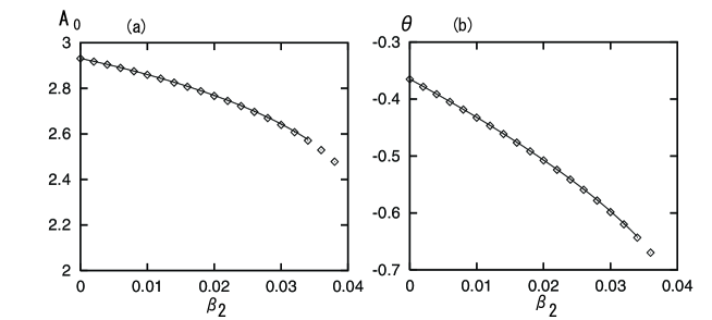
Figure 7: Comparison of the amplitude (a) and average phase (b) of the stable stationary periodic solutions, as found from the analytical approximation (continuous curves) and numerical solution (symbols). The dependences are obtained for the case $\beta_{2}=c_{2}$, the other parameters being fixed, with $k=-2$, $\gamma=1.5$, and the period $\Lambda=20/9$.

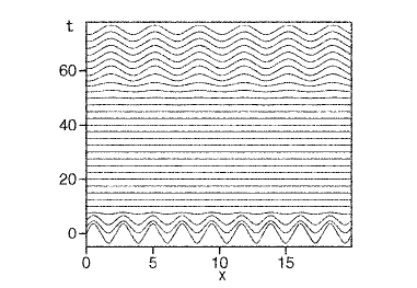
Figure 8: Time evolution of the real part of $u$ in the case with $c_{2}=\beta_{2}=0.045$, $k=-2,\gamma=1.5$. The period is $\Lambda=20/9$ in the initial state, and the period is $\Lambda=20/6$ in the final state.

2.2 Numerical results

The stationary version of eq. (7) was solved numerically, and the findings were compared to those obtained in the approximate analytical form based on eqs. (2) and (12). A typical example is displayed in Fig. 1, where the panel (a) shows the numerically found profile of $|u(x)|$ together with the analytical approximation to it, and the panel (b) is the corresponding phase profile, which was found only in the numerical form, as the analytical approximation assumes a constant phase.

Results for the stationary SP solutions can be summarized in the form of the plot displayed in Fig. 2. Its panel (a) shows the soliton’s amplitude, as found numerically and in the analytical approximation, vs. the coefficient $\beta_{2}=c_{2}$, which measures the deviation of the model (7) from the NLS counterpart (1), and the panel (b) shows the average value of the SP’s phase $\phi(x)$, which is defined as

$$\theta\equiv\frac{\int_{-\infty}^{+\infty}\phi(x)|u(x)|^{2}dx}{\int_{-\infty}^{+\infty}|u(x)|^{2}dx},$$ (16)

in comparison with the analytical prediction for the average phase, which is realized as the phase $\theta$ defined by eq. (12). The numerical and analytical results displayed in Fig. 2 terminate at points where, respectively, the numerical solution and eq. (12) cease to produce any nontrivial result (the numerical solution shows that, beyond the termination point, only the trivial state, $u=0$, can be found).

The results are further summarized in the diagram shown in Fig. 3, which displays a region in the parameter plane ($\beta_{2}=c_{2},k$), in which stable stationary SP solutions were found [the stability was verified by direct simulations of the full time-dependent equation (7)]. The upper right border marked by stars is the one beyond which only the zero solution can be found numerically; the dashed curve is an analytical prediction for the same border as given by eq. (13), i.e., the boundary beyond which eq. (12) yields no solutions. Below the lower border, which is marked by crosses, stable SPs cannot be found. The width of an initial pulse increases and the pulse spreads out to a spatially extended state. (The spatially extended state is not a uniform state.) The lower border is slightly upper than the instability line $k=\sqrt{\gamma^{2}-1}$ of the zero solution. The stability region in Fig. 3 ends approximately at $\left(\beta_{2}\right)_{{\rm cutoff}}\approx 0.16$, where the upper border approaches the lower border. Lastly, the upper left border, marked by rhombuses, is a line of the Hopf bifurcation destabilizing the SP: behind this border, a stable solution is a regularly or chaotically vibrating breather, see below.

The consideration of the above results, and the comparison with the analytical prediction shows that, first, the analytical approximation turns out to be fairly accurate, and, second, the stability region quickly shrinks with the increase of the diffusion and nonlinear-loss coefficients $\beta_{2}$ and $c_{2}$ in eq. (7). The stability region in Fig. 3 greatly extends in the direction of larger values of $k$ at small finite values of $\beta_{2}=c_{2}$ [which may be easily explained by the analytical result showing that the maximum value of $k$, as given by eq. (13), diverges as $\beta_{2}=c_{2}\rightarrow 0$].

Another relevant representation of the SP stability region is in terms of the parametric plane ($\beta_{1},k$) for fixed values $\beta_{2}=c_{2}=0.025,\,c_{1}=0.5$ and $\gamma=1.5$ of the other parameters, which is shown in Fig. 4. The two borders in Fig. 4 denote the same types of bifurcation curves as in Fig. 3. The upper border marked by stars is the one beyond which only the zero solution can be found numerically; the dashed curve is an analytical prediction $k_{{\rm cr}}=\{\gamma\sqrt{9+(8c_{2}+\beta_{2}/\beta_{1})^{2}}-3\}/(8c_{2}+\beta_{2}/\beta_{1})$, which is a modified one of eq. (13). The analytical prediction is good for large $\beta_{1}$, however, the approximation breaks down for small $\beta_{1}$, since the derivation of Eq. (13) is based on the conditions $\beta_{2}\ll\beta_{1}$ and $c_{2}\ll c_{1}$. Below the lower border, which is marked by crosses, stable SPs cannot be found. Note that the (unstable) exact SP solution (6) to the usual CCGL equation exists, unless both $\beta_{2}$ and $c_{2}$ vanish, not only at positive but also at negative values of the product $\beta_{1}c_{1}$ [10], which is a drastic difference from the classical NLS solitons that exist solely in the case $\beta_{1}c_{1}>0$. Nevertheless, Fig. 4 shows that the parametrically driven CCGL supports, as well as its NLS counterpart, (stable) SPs only in the case $\beta_{1}c_{1}>0$.

2.3 Breathers

As it was mentioned above, the SP solution suffers destabilization via the Hopf bifurcation at the border marked by rhombuses in Fig. 3, similar to what is known about solitons in the usual driven-NLS model 1 [7, 6, 8]. The Hopf bifurcation gives rise to stable oscillatory pulses in the form of breathers. Similar breathing pulses are also found in the quintic CCGL equation [17]. While we did not aim to investigate the breathers in detail, we have found that they always keep a single-humped shape. With further variation of the parameters, the breather performing regular oscillations undergoes period-doubling bifurcations, which do not destabilize the pulse as a whose, but render its intrinsic oscillations chaotic. Figure 5 shows the time evolutions of the breather’s amplitude, which is equal to $|u(L/2)|$, for $\gamma=1.5$ and $k=4.5$. The parameters $\beta_{1}$ and $c_{1}$ are again fixed to be 0.5. The amplitude of the pulse exhibits a limit cycle oscillation at $\beta_{2}=c_{2}=0.005$, a limit cycle oscillation with doubled period is seen at $\beta_{2}=c_{2}=0.002$, and the time evolution becomes chaotic at $\beta_{2}=c_{2}=0.001$.

3 Periodic waves

In the case when the condition (4) does not hold and the zero solution is unstable, SP solutions are irrelevant. However, it is natural to expect that the model supports spatially periodic stationary waves in this case, which may be quite relevant in the corresponding physical settings, provided that these waves are stable.

Periodic solutions can be first analyzed by means of an analytical approximation, similar to what was done above for the SP solutions, i.e., adopting the ansatz (8) with constant $\theta$. Then, an exact solution to the corresponding equation (9) is

$$u(x)=A_{0}\,{\rm cn}(\kappa x,q)e^{i\theta},$$ (17)

where ${\rm cn}$ is the elliptic cosine with the modulus $q=A_{0}/\sqrt{a^{2}+A_{0}^{2}}$, and other constants are defined as follows: $\kappa=\sqrt{(a^{2}+A_{0}^{2})/2}$, $A_{0}^{2}=2(k+\gamma\cos 2\theta)+\sqrt{4(k+\gamma\cos 2\theta)+2E}$, and $a^{2}=-2(k+\gamma\cos 2\theta)+\sqrt{4(k+\gamma\cos 2\theta)+2E}$. In these expressions, $E$ is a free parameter of the family of the periodic solutions, which can be fixed if a certain period $\Lambda$ is selected by periodic conditions. In terms of the above parameters,

$$\Lambda=4\sqrt{2}K(q)/\sqrt{a^{2}+A_{0}^{2}},$$ (18)

where $K(q)$ is the complete elliptic integral of the first kind.

To determine the value of $\theta$, we follow the same approach as in the case of SP, viz., we substitute the expression (17) into Eq. (11), then multiply it again by the expression (17), and integrate over the period (18). The resultant equation was solved numerically, in order to find $\theta$ for a given period $\Lambda$.

In a direct numerical simulation, we have obtained a stable pattern with the period $\Lambda=20/9$ at $c_{2}=\beta_{2}=0.02$, $k=-2$ and $\gamma=1.5$. In Fig. 6, we compare the direct numerical solution and the predicted approximate analytical solution for the periodic wave. A more general comparison of the analytical and numerical results is presented in Fig. 7, cf. a similar picture for the SP solutions in Fig. 2 [the average phase shown in Fig. 7(b) is defined by the expression (16), in which the integration is limited to one period of the solution; in fact, the phase of the periodic solution is almost constant, unlike that of SPs]. The dependences in Fig. 7 terminate at points beyond which the numerical solutions could not be continued. As concerns the numerical solution, in the case shown in Fig. 7, a solution with $\Lambda=20/9$ cannot be found for $\beta_{2}>0.04$. Figure 8 displays a time evolution at $\beta_{2}=c_{2}=0.045$. The initial condition is the periodic solution with the period $\Lambda=20/9$ for $\beta_{2}=c_{2}=0.02$ shown in Fig. 6. The amplitude of the periodic solution with the period $\Lambda=20/9$ decays to zero, and another periodic solution with period $\Lambda=20/6$ appears as a stable solution.

4 Conclusion

In this work, we have introduced a model of the one-dimensional nonlinear dispersive medium with intrinsic loss, which are compensated by a parametric driving field. The model is a combination of the parametrically driven nonlinear Schrödinger (NLS) and complex cubic Ginzburg-Landau equations, and has various physical applications (in particular, to optical systems). In the case when the zero background is stable, we developed an analytical approximation for a solitary-pulse (SP) solution, which was found to be in good agreement with direct numerical results. Unlike the well-studied case of the driven damped NLS equation, in the present case SPs have a nontrivial phase structure. Combining the analytical and numerical methods, we have identified the stability domain for the SP solutions. Generally, the increase of the diffusion and nonlinear-loss parameters leads to shrinkage of the stability region, but a nontrivial feature is that it may stretch in the direction of large values of the frequency mismatch. At one border of the stability domain, the SP is destabilized by the Hopf bifurcation, which gives rise to a localized breather. Further period doublings make internal vibrations of the breather chaotic. In the case when the zero background is unstable, hence SPs are irrelevant, we constructed stationary periodic solutions, for which a very accurate analytical approximation was developed, and their stability was studied in direct simulations.

References

- [1] H. Yamazaki and M. Mino, Progr. Theor. Phys. Suppl. 98 (1989) 400.
- [2] V.E. Zakharov, S.I. Musher, and A.M. Rubenchik, Phys. Rep. 129 (1985) 185; N. Yajima and M. Tanaka, Progr. Theor. Phys. Suppl. 94 (1988) 138.
- [3] J. Wu, R. Keolian, and I. Rudnick, Phys. Rev. Lett. 52 (1984) 1421; J. Miles and D. Henderson, Ann. Rev. Fluid Mech. 22, (1990) 143.
- [4] W.J. Firth, G.K. Harkness, A. Lord, J.M. McSloy, and D. Gomila, J. Opt. Soc. Am. B 19 (2002) 747.
- [5] J.W. Miles, J. Fluid Mech. 148 (1984) 451.
- [6] I.V. Barashenkov, M. M. Bogdan, and V.I. Korobov, Europhys. Lett. 15 (1991) 113.
- [7] A. Okamura and H. Konno, J. Phys. Soc. Jpn. 58, (1989) 1930.
- [8] M. Bondila, I.V. Barashenkov, and M.M. Bogdan, Physica D 87 (1995) 314; N.V. Alexeeva, I.V. Barashenkov, and D.E. Pelinovsky, Nonlinearity 12 (1999) 103.
- [9] L.M. Hocking and K. Stewartson, Proc. Roy. Soc. London 326, (1972) 289.
- [10] N.R. Pereira and L. Stenflo, Phys. Fluids 20, (1977) 1733.
- [11] A. Hasegawa and Y. Kodama. Solitons in Optical Communications (Oxford University Press: Oxford, 1995).
- [12] I.S. Aranson and L. Kramer, Rev. Mod. Phys. 74 (2002) 99.
- [13] B.A. Malomed, M. Gölles, I.M. Uzunov, and F. Lederer, Physica Scripta 55 (1997) 73.
- [14] H. Sakaguchi and B.A. Malomed, Physica D 167 (2002) 123.
- [15] M. Higuera, J. Porter, and E. Knobloch, Physica D 162 (2002) 155.
- [16] T. Mizuguchi and S. Sasa, Prog. Theor. Phys. 89 (1993) 599.
- [17] R.J. Deissler and H.R. Brand, Phys. Rev. Lett. 72 (1994) 478.