Wavefunction Statistics using Scar States

Abstract

We describe the statistics of chaotic wavefunctions near periodic orbits using a basis of states which optimise the effect of scarring. These states reflect the underlying structure of stable and unstable manifolds in phase space and provide a natural means of characterising scarring effects in individual wavefunctions as well as their collective statistical properties. In particular, these states may be used to find scarring in regions of the spectrum normally associated with antiscarring and suggest a characterisation of templates for scarred wavefunctions which vary over the spectrum. The results are applied to quantum maps and billiard systems.

School of Mathematical Sciences, University of Nottingham, Nottingham NG7 2RD, UK.

1 Introduction

The observation that random matrix theory (RMT) describes the statistical properties of the eigensolutions of a classically chaotic quantum system [1] has formed a pivotal role in our understanding of such systems. The most basic prediction for eigenfunctions is that they form a Gaussian distribution when projected on a generic state. More explicitly, the overlap between a generic probe state $|{\varphi}\rangle$ and the eigenstates $|{\psi_{n}}\rangle$ of the chaotic system has the probability distribution function

$$P(x)=\frac{1}{\sqrt{2\pi}}\;e^{-x^{2}/2},$$ (1)

where we normalise the states $|{\psi_{n}}\rangle$ so that the overlap $x=\langle{\varphi}|{\psi_{n}}\rangle$ has unit variance and assume time-reversal invariance for ease of notation. This distribution has been shown to work very accurately for billiard systems, for example [2].

In any such comparison with RMT statistics, deviations due to short time dynamics and other system-specific effects are particularly interesting. In systems such as quantum dots [3, 4], for example, such deviations may help us distinguish between RMT statistics arising from a simple underlying chaotic dynamics and RMT statistics which arise simply because the system is complex, perhaps dominated by interactions etc. In the context of wavefunction statistics, a remarkably strong example of such deviation has been demonstrated by Kaplan, Heller and coworkers [5, 6, 7]. They find that wavefunction statistics around a periodic orbit of the classical limit can deviate strongly from (1), an effect attributed to the phenomenon of scarring [8, 9, 10, 11] (whereby wavefunctions of classically chaotic systems are seen frequently to behave atypically near periodic orbits). These deviations can be robust and survive the semiclassical limit if the probe state $|{\varphi}\rangle$ is sufficiently localised in phase space around a periodic orbit. In this paper we describe the collective statistics of many components of the wavefunction using a basis of probe states which are locally complete near a periodic orbit. We find that a particular set of probe states can be defined in terms of which these deviations may be described particularly simply and these are related to states which have previously been used to characterise scarring under different guises ([5, 6, 7] and [12, 13, 14, 15, 16]), known variously under the names of universal test states [6], scarfunctions [14] or simply quasimodes [16].

The first theoretical explanation for scarring [9] was based on the evolution of a Gaussian wavepacket launched on a classical periodic orbit. Fourier analysis of the evolving wavepacket shows that typical overlaps of the wavepacket with chaotic eigenstates $\psi_{n}$ fluctuate quasiperiodically as a function of energy. Peaks occur in scarred parts of the spectrum associated with enhanced wavefunction probabilities near the periodic orbit and troughs are found in the antiscarred parts where wavefunctions are expected to be suppressed near the periodic orbit. More recently this basic idea has been developed further by Kaplan et al [5, 6, 7] to produce a quantitative theory of wavefunction statistics near a periodic orbit.

Kaplan et al consider the statistics of overlap with a single probe state $|{\varphi}\rangle$, which might typically be Gaussian. By considering quantum recurrence for such a state launched on a periodic orbit, one can show that the variance of the distribution $p(x)$ must deviate from the constant value predicted by RMT and is a function of the spectral parameter — energy $E$ in the case of time-independent systems and eigenangle $0\leq\theta<2\pi$ in the case of quantum maps. The overlap distribution in (1) is then naturally replaced by

$$P(x;\theta)=\frac{1}{\left[2\pi C(\theta)\right]^{1/2}}\;e^{-x^{2}/2C(\theta)},$$ (2)

where we adopt the notation of eigenangle for the spectral parameter and where the variance $C(\theta)$, which may be calculated from the linearised autocorrelation function of the probe state, is independent of $\hbar$.

This was generalised in [17] to provide a joint-probability distribution describing the statistics of the wavefunction in a basis of probe states which are complete in a neighbourhood in phase space of the periodic orbit. A minimum-uncertainty Gaussian wavepacket can be thought of as the ground state of a harmonic-oscillator Hamiltonian. We can also use as probe states the excited states $|{\varphi_{k}}\rangle$ of the same Hamiltonian and thereby obtain a series of overlaps ${\bf x}=(x_{0},x_{1},\cdots,x_{k},\cdots)$ representing the components of a chaotic eigenfunction in the harmonic-oscillator basis. (We adopt notation here appropriate to a single degree of freedom transverse to the periodic orbit, but it should be clear how to generalise these statements to higher dimensions.) One can then derive a matrix of correlations ${\bf C}(\theta)$ with components

$$C_{kl}(\theta)=\left\langle{x_{k}x_{l}}\right\rangle$$

which depends as before on the spectral parameter $\theta$ and which is independent of $\hbar$ (and therefore survives the semiclassical limit). The corresponding normal joint-probability distribution for the overlap amplitudes

$$P({\bf x};\theta)=\frac{1}{\left[(2\pi)^{M+1}{\rm det}\,{\bf C}(\theta)\right]^{1/2}}\;e^{-{\bf x}^{T}{\bf C}^{-1}(\theta)\,{\bf x}/2}$$ (3)

has been shown in [17] to describe well the statistics of eigenstates of perturbed cat maps and to lead to a quantitative understanding of the influence of scarring on the statistics of tunnelling from chaotic potential wells. The distribution has been written for a finite number of components $(x_{0},x_{1},\cdots,x_{M})$. The statistics of probe states sufficiently localised near the periodic orbit (but otherwise arbitrary) can straightforwardly be obtained from the limit $M\to\infty$. More generally though, this limit needs to be treated carefully, as discussed in Section 2.

In this paper we investigate the local structure of scarred eigenfunctions by using the envelope matrix ${\bf C}(\theta)$ to define a series of probe states adapted to a given periodic orbit and a given part of the spectrum. These scar states are defined so that the joint-probability distribution $P({\bf x};\theta)$ predicts statistical independence for their overlaps with chaotic wavefunctions. In a phase-space representation, these probe states are concentrated along the stable and unstable manifolds of the periodic orbit. In a region of the spectrum associated with maximal scarring, the first of these states corresponds to the scarfunction introduced by Vergini and Carlo in [14]. Elsewhere they correspond to linearised eigenstates such as considered by Nonnenmacher and Voros [13] and Kaplan and Heller [6]. The analysis here suggests an extension to a series of such states, however, forming a local basis near the periodic orbit. Furthermore these scar states vary as a function of the spectral parameter so that the local basis varies quasiperiodically as the spectrum is traversed. A surprising outcome, which has previously been noted in [6], is that in antiscarred regions of the spectrum, where conventionally we expect the chaotic wavefunction to be suppressed in a neighbourhood of the periodic orbit, we can define probe states for which chaotic wavefunctions have larger overlaps than predicted by RMT. That is, we find positive scarring in the antiscarred regions. We see in this paper that this observation generalises to a basis of such states, in terms of which a statistical description of wavefunction overlaps can be achieved using a simple product of independent Gaussians.

The organisation of the paper is as follows. In Section 2 we start by recalling the definition of the envelope matrix ${\bf C}(\theta)$ and then we define optimised probe states which give decoupled overlap distributions with scarred eigenfunctions. We also discuss the local pattern of the scarred eigenfunctions and how these vary with the spectral parameter $\theta$. We see how this works for a specific quantum map model in Section 3 and we consider billiard systems in Section 4, where we show that the statistics of the boundary eigenfunctions can also be described by the joint-probability distribution $P({\bf x};\theta)$.

2 The envelope matrix and scar states

In this section we begin with a brief description of the envelope matrix ${\bf C}(\theta)$ which determines the joint-probability distribution $P({\bf x};\theta)$. The eigenvectors of ${\bf C}(\theta)$ can be interpreted as providing the statistically independent basis for the joint-probability distribution. The eigenvectors with the largest eigenvalues provide us with probe states which give overlap distributions in which the effect of scarring is optimised. Borrowing the terminology of Vergini and Carlo, we refer to these probe states as scar states. We show in particular that the first of these scar states coincides in the semiclassical limit with the scarfunction introduced by Vergini and Carlo [14] and that in general they form a subset of the hyperbolic stationary states whose coherent-state representations have been described in detail by Nonnenmacher and Voros [13].

The notation in this section is adapted to the case of a quantum map $\hat{U}$ with eigensolutions $\hat{U}|{\psi_{n}}\rangle=e^{-i\theta_{n}}|{\psi_{n}}\rangle$. We consider statistics of ensembles which are constructed by restricting the eigenangle $\theta_{n}$ to a narrow window centred at the value $\theta$. The corresponding construction in the case of time-independent systems is to consider states for which the action $S(E_{n})$ of the periodic orbit under consideration is such that $\theta_{n}=S(E_{n})/\hbar$ is similarly restricted.

2.1 Envelope matrix ${\bf C}(\theta)$

The joint-probability distribution $P({\bf x};\theta)$ completely characterises the influence of scarring on wavefunction statistics near the periodic orbit and our assertion is that this is in turn completely determined (to a good approximation at least) by the envelope matrix ${\bf C}(\theta)$. For a given periodic orbit, the matrix ${\bf C}(\theta)$ is constructed in practice from a Fourier transform of a correlation matrix ${\bf A}(t)$, formed by writing linearised quantum evolution in a harmonic-oscillator basis $\{|{\varphi_{k}}\rangle\}$. For simplicity of notation, let us assume that the periodic orbit is in fact a fixed point $p_{0}$ of a chaotic map and that this map is quantised by the unitary operator $\hat{U}$, while $\hat{U}_{\rm lin}$ quantises the linearised dynamics around $p_{0}$. The matrix ${\bf A}(t)$ is simply $\hat{U}_{\rm lin}^{t}$ written in the basis $\{|{\varphi_{k}}\rangle\}$, with elements

$$A_{kl}(t)=\langle{\varphi_{k}}|\hat{U}^{t}_{{\rm lin}}|{\varphi_{l}}\rangle.$$ (4)

We might of course use any basis of states localised in phase space around $p_{0}$ but we use a harmonic oscillator basis because we can then write closed-form expressions for $A_{kl}(t)$. These are given explicitly in Appendix A, but here we simply note the essential features.

The linearised evolution underlying $\hat{U}_{\rm lin}$ has inversion through $p_{0}$ as a symmetry (even if the full map $\hat{U}$ does not) and this leads to a decoupling of ${\bf{A}}(t)$ into blocks corresponding to even and odd values of $k$. That is, $A_{kl}(t)=0$ unless $k$ and $l$ are both even or both odd. In any discussion of statistics it is therefore natural to consider separately the components $x_{k}$ for even and odd $k$ — any explicit calculation we give will be for the even case. The linearised evolution also has a time-reversal symmetry (again, even if the full map $\hat{U}$ does not). This means that we can choose phases of $|{\varphi_{k}}\rangle$ so that ${\bf{A}}(t)$ is symmetric and $\left({\bf{A}}(t)\right)^{*}={\bf{A}}(-t)$.

For a map with one degree of freedom, two classical parameters which characterise the classical situation are sufficient to determine ${\bf{A}}(t)$. The first of these is the stability eigenvalue $\lambda^{t}=\pm e^{\rho t}$ of the unstable dynamics around $p_{0}$. This sets the rate at which ${\bf{A}}(t)$ decays with $t$ and subsequently the strength of deviations due to scarring. The second parameter effectively characterises the harmonic-oscillator basis. Any elliptic linear evolution which has $p_{0}$ as a fixed point can be used to generate a harmonic-oscillator basis $|{\varphi_{k}}\rangle$, and we should expect ${\bf{A}}(t)$ to depend on the eccentricity and orientation of this elliptic evolution (relative to the hyperbolic structure of the unstable dynamics around $p_{0}$). It turns out that a single parameter, which we denote $Q$ following Kaplan and Heller, is sufficient to completely characterise this dependence, and is easily interpreted geometrically. Let $(q,p)$ be canonical coordinates for which the harmonic oscillator defining $|{\varphi_{k}}\rangle$ is a multiple of $q^{2}+p^{2}$. Then $Q=\cot\alpha$, where $\alpha$ is the angle in coordinates $(q,p)$ between the stable and unstable manifolds of the chaotic dynamics about $p_{0}$.

The expressions for ${\bf A}(t)$ given in Appendix A are simplest for the case $Q=0$, which corresponds to orthogonal stable and unstable manifolds (relative to the coordinates $(q,p)$ suggested by the normal form for the harmonic oscillator). If we are interested in the wavefunction statistics in isolation, then the basis $|{\varphi_{k}}\rangle$ may be chosen at our convenience and it seems natural in that case to ensure that $Q=0$. In applications to tunnelling statistics [17], however, the basis $|{\varphi_{k}}\rangle$ is imposed by a secondary calculation and it is therefore useful to be able to treat the case $Q\neq 0$. We will also find this option convenient when we apply the results to an explicit model in the next section.

Given ${\bf A}(t)$, we define the envelope matrix by

$${\bf C}(\theta)=\sum_{t=-\infty}^{\infty}e^{i\theta t}{\bf{A}}(t).$$

Given the properties of ${\bf{A}}(t)$ described above, this is a real symmetric matrix which decouples into even and odd blocks. If we construct an ensemble of chaotic eigenstates $|{\psi_{n}}\rangle$ from a small window around the spectral parameter $\theta$, modulo $2\pi$, then it can be shown that the components $C_{lk}(\theta)$ give the averages $\left\langle{x_{l}^{*}x_{k}}\right\rangle$ [17]. Given such an RMT-violating constraint on variance and correlation, a common procedure in the analysis of wavefunction statistics has been to assert that the statistical distribution remains normal but with an appropriately adjusted covariance matrix. In particular, this has been done by Antonsen et al [18] for averages of the wavefunction along the periodic orbit and by Narimanov et al [3] for the wavefunction itself. In our case this amounts to assuming the joint probability distribution (3) in the case of GOE statistics, with an obvious generalisation for the GUE case. While we cannot prove the result, the distribution was shown in [17] to successfully describe the statistics of low-lying components of ${\bf x}$ and to explain deviations due to scarring of tunnelling-rate statistics. We posit the result simply as a conjecture and refer to the numerical evidence presented here and in [17] as justification for it.

The joint-probability distribution obtained from ${\bf C}(\theta)$ is written in (3) for a truncated set of components $({\bf x}=x_{0},x_{1},\cdots,x_{M})$. To obtain a complete characterisation of wavefunction statistics, we should take a limit $M\to\infty$. However, because ${\bf C}(\theta)$ is derived from a linearised hyperbolic system whose quantisation does not have normalised eigenstates, the elements of ${\bf C}(\theta)$ decay quite slowly and the limit must be treated with care. We find a straightforward limit if we use (3) to obtain the statistics of a measure such as

$$\xi_{n}=\langle{\psi_{n}}|{\hat{P}}|{\psi_{n}}\rangle$$ (5)

which samples the chaotic state $|{\psi_{n}}\rangle$ in a localised region of phase space around $p_{0}$. Localisation in the context of (5) means that $\hat{P}$ is an operator whose matrix representation ${\bf P}$ in the harmonic-oscillator basis decays sufficiently rapidly that ${\rm Tr}\,{\bf P}{\bf C}(\theta)$ exists — it has been shown in [17] that the statistics of $\xi_{n}$ are then governed by a distribution of the form (assuming GOE statistics and Hermitian $\hat{P}$)

$$p(\xi;\theta)=\frac{1}{2\pi}\int\frac{e^{-iqy}}{\sqrt{{\rm det}\,\!\!\left(1+2iq{\bf P}{\bf C}(\theta)\right)}}\;{\rm d}q,$$ (6)

that is well-defined in the limit $M\to\infty$. Alternatively, any finite subset of the components ${\bf x}=(x_{0},x_{1},\cdots)$ can be described by a joint-probability distribution written analogously to (3) with an appropriate submatrix of ${\bf C}(\theta)$. The limit $M\to\infty$ is not simple however, if we try to treat $P({\bf x};\theta)$ as a full distribution.

2.2 The construction of scar states

Consider the distribution for a finite set of coordinates ${\bf x}=(x_{0},x_{1},\cdots,x_{M})$. As for any normal distribution it is natural to rotate these coordinates so as to produce a statistically independent basis ${\bf y}=(y_{0},y_{1},\cdots,y_{M})$ for which

$$\left\langle{y_{i}y_{j}}\right\rangle=s_{i}(\theta)\delta_{ij}$$ (7)

and for which the joint-probability distribution is a simple product of Gaussian distributions,

$$P({\bf y};\theta)=\prod_{i=0}^{M}P(y_{i};\theta)=\prod_{i=0}^{M}\frac{1}{\sqrt{2\pi s_{i}(\theta)}}\;e^{-y_{i}^{2}/2s_{i}(\theta)}.$$ (8)

These are obtained as the eigenvectors and eigenvalues of the corresponding $(M+1)\times(M+1)$ submatrix of ${\bf C}(\theta)$. It should be noted, however, that because the infinite-dimensional limit of ${\bf C}(\theta)$ does not have proper eigenvectors, the coordinates $y_{i}$ and the eigenvalues

$${\bf s}(\theta)\equiv(s_{0}(\theta),s_{1}(\theta),\cdots,s_{M}(\theta)),$$

do not converge in a simple way as $M\to\infty$. We will see in particular that the leading eigenvalues diverge logarithmically with increasing $M$. This means that we can construct linear combinations of the harmonic-oscillator basis states $|{\varphi_{k}}\rangle$ for which the overlaps with the chaotic states $|{\psi_{n}}\rangle$ can be made arbitrarily large, on average, compared with the expectation from RMT. It should be noted however that for any finite value of $\hbar$ there is a limit to how large we can let $M$ become without the linear approximation underlying the construction of ${\bf C}(\theta)$ becoming invalid and the limit $M\to\infty$ can therefore only sensibly be taken in conjunction with the semiclassical limit [19].

We begin by deriving formally the eigenvectors of ${\bf C}(\theta)$ in an infinite basis and later indicate how these solutions are regularised by truncation. For this purpose we use the fact that ${\bf{A}}(t)$ and ${\bf C}(\theta)$ decompose into even and odd blocks and consider these blocks, denoted by ${\bf{A}}^{\pm}(t)$ and ${\bf C}^{\pm}(\theta)$, separately. Using Poisson resummation we write

$${\bf C}^{\pm}(\theta) = \sum_{m=-\infty}^{\infty}\int_{-\infty}^{\infty}e^{i(\theta+2\pi m)t}{\bf{A}}^{\pm}(t)\,{\rm d}t$$ (9)

$$= \sum_{m=-\infty}^{\infty}{\bf F}^{\pm}(\theta+2\pi m)$$

and we claim that

$${\bf F}^{\pm}(\Omega)=\int_{-\infty}^{\infty}e^{i\Omega t}{\bf{A}}^{\pm}(t)\,{\rm d}t$$

is an unnormalised projection onto an eigenvector of ${\bf C}^{\pm}(\theta)$ if $\Omega=\theta+2\pi m$ for some integer $m$. We see this by writing

$$F_{kl}^{\pm}(\Omega)=\langle{\varphi_{k}}|{\hat{S}(\Omega)}|{\varphi_{l}}\rangle,$$

where the superscript $\pm$ indicates whether $|{\varphi_{k}}\rangle$ and $|{\varphi_{l}}\rangle$ are restricted to the even or odd subspaces and $\hat{S}(\Omega)$ is the operator

$$\hat{S}(\Omega)=\int_{-\infty}^{\infty}e^{i\Omega t}\,{\hat{U}_{\rm lin}^{t}}\,{\rm d}t.$$

Let us now substitute

$$\hat{U}_{\rm lin}^{t}=e^{-i\hat{H}t/\hbar}$$

where $\hat{H}$ is a quadratic Hamiltonian linearising the hyberbolic dynamics about $p_{0}$. We expand

$$\hat{U}_{\rm lin}^{t}=\sum_{\pm}\int{\rm d}E\,e^{-iEt/\hbar}\,|{E^{\pm}}\rangle\langle{E^{\pm}}|$$

in eigenbasis $\hat{H}|{E^{\pm}}\rangle=E|{E^{\pm}}\rangle$ of $\hat{H}$, with the usual normalisation $\langle{E^{\pm}}|{{E^{\prime}}^{\pm}}\rangle=\delta(E-E^{\prime})$. The sum over $\pm$ here arises because the eigenstates for each $E$ are doubly-degenerate. In a representation where the problem amounts to scattering from a parabolic barrier, the conventional description of this degeneracy is in terms of scattering states with left or right incoming waves, but in our case we choose eigenstates that have even or odd parity. This decomposition gives in turn that

$$\hat{S}(\Omega)=2\pi\delta(\Omega-\hat{H}/\hbar)=2\pi\hbar\sum_{\pm}|{E(\Omega)^{\pm}}\rangle\langle{E(\Omega)^{\pm}}|$$

where $E(\Omega)=\hbar\Omega$. We note that phase space representations of the states $|{E^{\pm}}\rangle$ have been analysed in detail by Nonnenmacher and Voros [13] (beware however that in their notation the label $\pm$ sometimes refers to the direction of an incoming wave whereas here it always refers to parity) and we will return to their phase-space description later. This formal result states simply that the eigenvectors of ${\bf C}^{\pm}(\theta)$ are representations in the harmonic-oscillator basis of the subset of these states for which $\Omega=\theta+2\pi m$ and which have a definite parity. In particular we may decompose ${\bf C}^{\pm}(\theta)$ as promised in (9), with

$${\bf F}^{\pm}(\Omega)=2\pi\hbar\,{\bf w}^{\pm}(\Omega)\,{\bf w}^{\pm}(\Omega)^{\dagger}$$ (10)

and $w_{k}^{\pm}(\Omega)=\langle{\varphi_{k}}|{E(\Omega)^{\pm}}\rangle$.

Equation (9) therefore provides us formally with a spectral decomposition of ${\bf C}^{\pm}(\theta)$ with eigenvectors ${\bf w}^{\pm}(\theta+2\pi m)$ labelled by the integers $m$. The corresponding eigenvalues diverge, however, because the hyperbolic stationary states $|{E^{\pm}}\rangle$ are unnormalisable. This supports our earlier assertion that the eigenvalues of a finite submatrix of ${\bf C}(\theta)$ diverge as $M\to\infty$. To regularise the situation we must consider truncations of ${\bf C}(\theta)$. This corresponds physically to restricting the probe states we use to be sufficiently localised near $p_{0}$ in phase space, which is in any case a necessity if the linearised evolution used in deriving the form of ${\bf{A}}(t)$ is to be valid.

We will consider truncations of the form

$$\tilde{C}_{kl}(\theta)=\sqrt{P_{k}}C_{kl}(\theta)\sqrt{P_{l}}$$

where the coefficients $P_{k}$ decay from unity sufficiently rapidly that $\tilde{{\bf C}}(\theta)$ has a series of nonvanishing eigenvalues with normalisable eigenvectors, but sufficiently slowly that $\tilde{{\bf C}}(\theta)$ can be regarded as an approximation for ${\bf C}(\theta)$ in an appropriate neighbourhood of $p_{0}$. In the simplest case we use a step function $P_{l}=\Theta(M-l)$, which replaces ${\bf C}(\theta)$ with a finite submatrix describing the statistics of $(x_{0},x_{1},\cdots,x_{M})$, but we may also let $P_{k}$ decay smoothly. This truncation is useful in the statistics of (5) above in the case $\hat{P}=\sum_{k}P_{k}|{\varphi_{k}}\rangle\langle{\varphi_{k}}|$ (which is the form seen in applications to tunnelling, where $P_{k}$ is a tunnelling rate associated with the probe state $|{\varphi_{k}}\rangle$). In particular we will use truncating functions of the form

$${P}_{k}=\frac{1}{{1+e^{\beta(k-M)}}},$$ (11)

where $M$ behaves as a cutoff in the dimension of $\tilde{{\bf C}}(\theta)$ and $\beta$ provides a decay rate after cutoff. The sharp truncation above corresponds to the limit $\beta\to\infty$.

Figure 1: The leading eigenvalues ${\bf s}(\theta)=(s_{0}(\theta),s_{1}(\theta),\cdots)$ of the envelope matrix $\tilde{{\bf C}}(\theta)$. Here we use truncation parameters $\beta=0.025$ and $M=300$. The bullets indicate $s_{i}(\theta)$ for $i=0,1$ and $2$ and for $\theta=-\pi/2,0,\pi/2$ and $\pi$. The Husimi distributions corresponding to these eigenvalues are shown in Figure 2.

The eigenvectors of the truncated matrix $\tilde{{\bf C}}(\theta)$ are not as straightforwardly calculated as those of the full matrix ${\bf C}(\theta)$. The leading eigenvectors, however, corresponding to smaller absolute values of $m$, should approximately coincide with those of ${\bf C}(\theta)$. In detail, if $E(\Omega)$ with $\Omega=\theta+2\pi m$ is small enough and the components of $\hat{P}$ decay slowly enough from unity then

$$\left(\sqrt{{\bf P}}{\bf w}^{\pm}(\Omega)\right)_{k}=\sqrt{P_{k}}w_{k}^{\pm}(\Omega)$$

is approximately an eigenvector of $\tilde{{\bf C}}(\theta)$ with eigenvalue

$$s(\Omega) = 2\pi\hbar\,(\sqrt{{\bf P}}{\bf w}^{\pm}(\Omega))^{\dagger}\sqrt{{\bf P}}{\bf w}^{\pm}(\Omega)$$

$$= 2\pi\hbar\,\langle{E(\Omega)^{\pm}}|{\hat{P}}|{E(\Omega)^{\pm}}\rangle.$$

Since $|{E(\Omega)^{\pm}}\rangle$ is unnormalisable, these eigenvalues diverge as promised as the truncation dimension increases and $\hat{P}\to I$. The eigensolution is only approximate because, while (10) still applies to the truncated matrix if ${\bf w}^{\pm}(\Omega)$ is replaced by $\sqrt{{\bf P}}{\bf w}^{\pm}(\Omega)$, the vectors $\sqrt{{\bf P}}{\bf w}^{\pm}(\Omega)$ for two different values of $\Omega$ are only approximately orthogonal.

We present in Figure 1 the leading eigenvalues, relabelled $(s_{0}(\theta),s_{1}(\theta),\cdots)$ in order of decreasing value, for a fixed point $p_{0}$ with stable and unstable manifolds along $p=\pm q$, a harmonic oscillator basis with $Q=0$ and using a smooth truncation of the form given in (11). As expected from the preceding discussion, these eigenvalues unfold to give a smooth function of $\Omega=\theta+2\pi m$, decreasing from the centre. The leading eigenvalue is peaked in the so-called scarred region of the spectrum — we have chosen phases so that this occurs at $\theta=0$. In terms of wavefunction statistics, this means that the corresponding eigenvector defines a probe state for which the variance is much larger than predicted by RMT (about 18 times larger for the parameters illustrated in Figure 1). The scarred region is also where overlap statistics of chaotic wavefunctions with a simple Gaussian probe state have the greatest variance. In the case of a Gaussian probe state, however, the variance falls between these peaks to a value significantly smaller than predicted by RMT in the anti-scarred region, corresponding here to the region around $\theta=\pi$ — this contrasts with the case where we track a probe state corresponding to the leading eigenvector, in which case the overlap statistics have large variances even in the anti-scarred region (albeit not as large as in the scarred region).

The leading eigenvalue $s_{0}(\theta)$ can be tracked through crossings in the antiscarred region to give the next eigenvalue $s_{1}(\theta)$ and so on. Although less dramatically deviant than the leading eigenvalue, these subsequent eigenvalues define probe states which also have overlaps that are significantly larger than predicted by RMT. As with the leading probe state, the overlaps they define are larger than RMT even in the antiscarred region. For any finite truncation dimension and increasing index, the eigenvalues will eventually become very sensitive to the truncation and will not define useful probe states. For a fixed index and increasing truncation dimension, however, the probes states provide us with a useful characterisation of wavefunctions near the periodic orbit and we will refer to these probe states as scar states.

We will see later that the leading eigenvalues increase logarithmically with the effective truncation dimension $M$. The leading eigenvectors, on the other hand, converge to give a meaningful limit in the region of phase space surrounding the periodic orbit. A detailed discussion for the Husimi distributions of such hyperbolic stationary states has been given in [13] and we illustrate these with some explicit cases here. Given an eigenvalue $s_{i}(\theta)$, we denote the corresponding scar state by $|{\chi_{i}(\theta)}\rangle$ which in the limit $M\to\infty$ approaches

$$|{\chi_{i}(\theta)}\rangle\to|{E(\theta+2\pi m_{i})^{\pm}}\rangle$$

for some integer $m_{i}$. We denote the corresponding Husimi distribution by

$$H_{i}(q,p;\theta)=|\langle{z}|{\chi_{i}(\theta)}\rangle|^{2}.$$ (12)

Figure 2 illustrates this Husimi distribution for some of the leading scar states, whose eigenvalues $s_{i}(\theta)$ are indicated by bullets in Figure 1. The scar states shown are appropriate to a fixed point $p_{0}$ at the origin of phase space with stable and unstable manifolds defined by $p=\pm q$. Each of these Husimi functions is strongly localised around the stable and unstable manifolds of the fixed point, although the details vary with the spectral parameter $\theta$ and index $i$. In distinguishing between different cases it is useful to note that the zeros of the Husimi functions are visible as dark spots — these enable us to distinguish between states which are concentrated in similar regions of phase space but which have different phase structure.

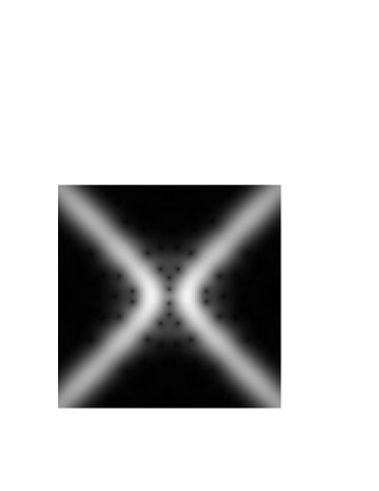
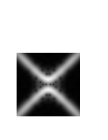
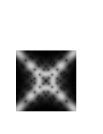
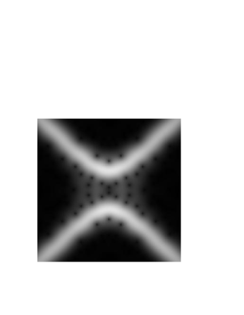
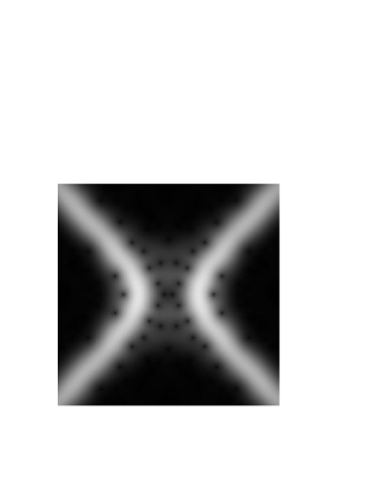
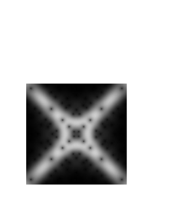
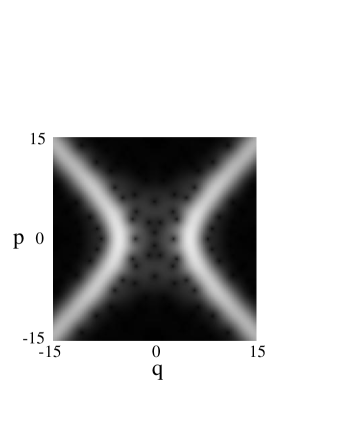
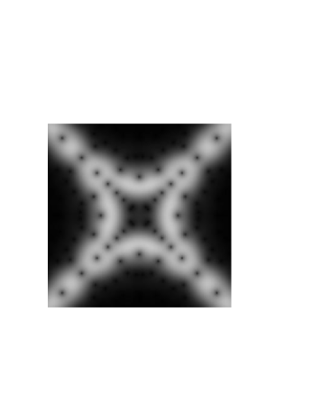
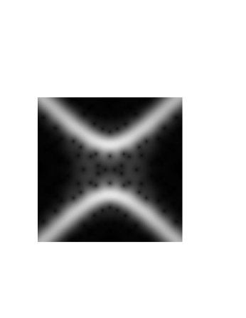
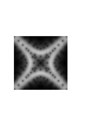
Figure 2: The Husimi functions of the scar states corresponding to the bullets in Figure 1. The underlying hyperbolic system has stable and unstable manifolds along the diagonals $p=\pm q$. The first row gives $H_{0}(q,p,\theta)$ for $\theta=-\pi/2,0,\pi/2$ and $\pi$. The second and third rows give $H_{1}(q,p,\theta)$ and $H_{2}(q,p,\theta)$ for the same values of $\theta$. Zeros of the Husimi functions appear as dark points.

The leading scar states $|{\chi_{i}(\theta)}\rangle$ are potentially useful not only for understanding the statistics of wavefunctions but also for characterising the structure of individual wavefunctions. The variance of the overlap $\langle{\chi_{i}(\theta)}|{\psi_{n}}\rangle$ is quite large and in fact can diverge in the semiclassical limit. In a given part of the spectrum, chaotic eigenfunctions will therefore tend to have especially large components along the corresponding scar states. One aspect of this is that we might therefore recognise the characteristics of the scar states in individual states, and the changing form of the scar states across the spectrum will provide a template for recognising such structures. We will see explicit examples of this in the next section. A second aspect is that the scar states should provide a powerful guide to choosing bases for the explicit calculation of chaotic eigenstates. This sort of construction has recently been proposed by Vergini and Carlo [20]. They have in particular defined for each periodic orbit a scarfunction which is concentrated around the stable and unstable manifolds much like the scar states $|{\chi_{i}(\theta)}\rangle$ are. In fact we will see in the next subsection that the scarfunction coincides with the leading state $|{\chi_{0}(0)}\rangle$ in the semiclassical limit. The property of the states $|{\chi_{0}(\theta)}\rangle$ that they change as a function of $\theta$ and adapt to a given part of the spectrum, as well as the ability to generate additional orthogonal states (labelled by $i$), might therefore provide a useful generalisation of that approach.

2.3 The leading scar state

We show now how the decomposition outlined in the previous subsection emerges in the harmonic-oscillator basis. We cannot give closed-form expressions for general scar states $|{\chi_{i}(\theta)}\rangle$ in this basis, but we can calculate the basic properties of the leading state $|{\chi_{0}(0)}\rangle$ in the scarred part of the spectrum, corresponding to $\theta=0$ in our convention. We will see in particular that this reproduces the scarfunction of Vergini and Carlo [14].

We have noted that the envelope matrix ${\bf C}(\theta)$ depends on the stability exponent $\rho$ of the underlying hyperbolic dynamics and a parameter $Q$ depending on the basis. We are free to choose a basis for which $Q=0$ and we assume that to be the case in this subsection. The stability exponent $\rho$ determines how quickly the correlation matrix ${\bf{A}}(t)$ decays with $t$ and therefore how far the envelope matrix ${\bf C}(\theta)$ deviates from the RMT case ${\bf C}(\theta)=I$. The eigenvalues ${\bf s}(\theta)$ in particular depend strongly on $\rho$. The scar states, however, depend only on the underlying geometry of the stable and unstable manifolds and not on the rate of decay. We therefore consider the limit $\rho\to 0$, which simplifies because we can then replace the Fourier series defining ${\bf C}(\theta)$ by an integral

$$\sum_{t}{\bf A}(t)e^{i\theta t}\longrightarrow\int\,{\bf A}(t)e^{i\theta t}\;{\rm d}t.$$ (13)

In other words, the sum in (9) is dominated by the $m=0$ term. We note that this formulation is similar to the construction of the universal scar measure in [6] or the continuous quasimode in [16], except here we also incorporate the propagation of excited harmonic-oscillator eigenstates as well as the Gaussian ground state.

Using the form for ${\bf A}(t)$ given in Appendix A we can in particular evaluate this integral explicitly for the case $\theta=0$. We find a decomposition of the form

$${\bf C}(0)\simeq\frac{1}{\rho}{\bf v}{\bf v}^{T},$$ (14)

where the components of the vector ${\bf v}$ are

$$v_{k}=\cases{\displaystyle(-1)^{n}(2\pi)^{-1/4}\frac{\sqrt{(4n)!}}{2^{2n}(2n)!}\frac{\Gamma(n+\frac{1}{2})}{\Gamma(n+\frac{3}{4})}&\quad for $k=4n$,\cr\vskip 12.0pt\cr\qquad\qquad 0&\quad otherwise.\cr&}$$ (15)

This means that ${\bf v}$ is the leading eigenvector of ${\bf C}(0)$ and that the corresponding eigenvalue is

$$s_{0}(0)\simeq\frac{1}{\rho}{\bf v}^{T}{\bf v}.$$ (16)

The vanishing of components $v_{k}$ for odd $k$ is a reflection of the fact that linearised evolution has inversion through the origin as a symmetry — we have already see that this symmetry leads in the general case to a decoupling of ${\bf C}(\theta)$ into odd and even blocks. When we choose a basis for which $Q=0$, the stable and unstable manifolds are orthogonal and we have in addition a symmetry of interchange $(q,p)\to(p,-q)$ of the corresponding canonical coordinates. this is responsible for a further decoupling of the index $k$ mod $4$. This four-fold symmetry is also reflected in the general case, in particular through the symmetry $H_{i}(q,p,\theta)=H_{i}(p,q,-\theta)$ visible in the Husimi functions of Figure 2.

We remark that this eigensolution depends on the stability exponent $\rho$ only through the prefactor in (16). The calculation has been performed formally for the untruncated matrix ${\bf C}(\theta)$ and we note that (16) is divergent and gives a meaningful eigenvalue only if we truncate the matrix at a finite dimension $M$. We can obtain an estimate for the divergence of $s_{0}(0)$ with truncation dimension by noting that the components of ${\bf v}$ have the asymptotic behaviour (as $k=4n\to\infty$)

$$v_{4n}^{2}\simeq\frac{1}{n}.$$

The leading eigenvalue for a matrix sharply truncated at dimension $M$ therefore asymptotes to (as $\rho\to 0$ and $M\to\infty$)

$$s_{0}(0)\simeq\frac{1}{\rho}\sum_{n=1}^{M/4}v_{4n}^{2}\simeq\frac{1}{\rho}\log(M/4)+{\rm const}.$$ (17)

Although our derivation has been restricted to the limit $\rho\to 0$, we remark that this describes quite well the divergence of $s_{0}(0)$ even for moderate values of $\rho$, as indicated in Figure 3 where we compare it with a numerical calculation for $\rho=0.6$.

Figure 3: The leading eigenvalue $s_{0}(0)$ as a function of the sharp cut-off dimension $M$ when $\rho=0.6$ and $Q=0$, showing a logarithmic divergence. The solid curve is the approximation in (17).

We expect similar divergence to hold for the next-to-leading eigenvalues. Since $s_{i}(\theta)$ diverges we might then expect to be able to make the statistical deviation from RMT arbitrarily large by choosing appropriate probe states. It should be noted, however, that our results are meaningful only if we take the limit $M\to\infty$ in conjunction with the semiclassical limit $\hbar\to 0$. Our calculation of the correlation $C_{kl}(\theta)$ between two basis states was obtained by assuming evolution that is linearised about the periodic orbit. This is always valid for fixed $k$ and $l$ in the semiclassical limit. If we fix $\hbar$ and take the limit $k,l\to\infty$, however, the basis states $|{\varphi_{k}}\rangle$ will eventually fall outside the region of phase space where the linearisation is appropriate and the correlations $C_{kl}(\theta)$ will then not accurately describe the statistics. For any given quantum system then, we should restrict ourselves to truncations for which linearised evolution is accurate and this effectively limits the value of $s_{i}(\theta)$ and therefore the deviation from RMT.

Consistent with the preceding subsection, the vector ${\bf v}$ can also be expressed formally as an eigenstate of the Hamiltonian

$$\hat{H}=\frac{\rho}{2}(p^{2}-q^{2})$$ (18)

giving the underlying hyperbolic motion in appropriate canonical coordinates $(q,p)$. We can express this Hamiltonian in terms of creation and annihilation operators of a harmonic oscillator basis for which $Q=0$ as

$$\hat{H}=-\frac{\rho}{2}({a^{\dagger}}^{2}+a^{2}).$$

The vector ${\bf v}$ is then easily seen formally to be a null eigenvector

$${\bf H}{\bf v}=0$$ (19)

of the Hamiltonian matrix

$$({\bf H})_{kl}\equiv\langle{\varphi_{k}}|{\hat{H}}|{\varphi_{l}}\rangle.$$

In particular the leading scar state is also one of the simpler cases for which Husimi functions were constructed in [13]. This can be seen by using the representation

$$|{z}\rangle=e^{-|z|^{2}/2}\sum_{k=0}^{\infty}\frac{1}{\sqrt{k!}}{z^{*}}^{k}|{\varphi_{k}}\rangle$$

of the coherent states, where $z=(q-ip)/\sqrt{2\hbar}$, and substituting the coefficients of (15) in (12), giving

$$H_{0}(z,0) = \frac{1}{\sqrt{2\pi}}\,e^{-|z|^{2}}\left|\sum_{n=0}^{\infty}(-1)^{n}\frac{\Gamma(n+\frac{1}{2})}{\Gamma(n+\frac{3}{4})}\frac{z^{4n}}{2^{2n}(2n)!}\right|^{2}$$

$$= \frac{1}{2}\sqrt{\frac{\pi}{2}}e^{-|z|^{2}}\left|\sqrt{z}J_{-1/4}\left(\frac{z^{2}}{2}\right)\right|^{2}$$

for the Husimi function of this state. This coincides with the expression in [13] for the $E=0$ eigenstate of the hyperbolic system as expected from the discussion of the previous subsection.

The preceding discussion also helps us to relate $|{\chi_{0}(0)}\rangle$ to the scarfunction of Vergini and Carlo [14]. They define the scar function $|{\chi}\rangle$ to be a finite linear combination of the states $|{\varphi_{k}}\rangle$ which minimises

$$\langle{\chi}|{\hat{H}^{2}}|{\chi}\rangle.$$

In the limit $M\to 0$ the eigenvector ${\bf v}$ provides a solution to just this problem and the corresponding state $|{\chi_{0}(0)}\rangle$ should therefore coincide with the scarfunction of [14] in that limit.

Away from the scarred region, that is for $\theta\neq 0$, the scar states should correspond to universal test states [6, 15], or quasimodes [16], although we have not written explicit forms for them in a harmonic-oscillator representation. Note however that one can find explicit expression for the Husimi functions in [13]. We also note that phase space representations of operators with the structure of $\tilde{{\bf C}}(\theta)$ have also been given by Rivas and Ozorio de Almeida [21], and these might also be useful in deriving explicit expressions for the scar states in phase space.

3 Application to a quantum map model

We now investigate how well the scar states describe wavefunction structure and statistics for a specific quantum map model. The details of this model are unimportant and we merely remark that the classical system is a hyperbolic mapping of the torus with time-reversal symmetry and a fixed point at the origin — the detailed parameters for the system are the same as those given in [17] and the reader should look there for further details. As in [17], we choose as basis states $|{\varphi_{k}}\rangle$ the eigenstates of a Harper Hamiltonian which is harmonic near the fixed point. This problem is characterised by a stability exponent $\rho=0.6006$ and a basis-parameter $Q=0.5658$. The semiclassical limit is controlled by the dimension of Hilbert space, which we denote by $N$. Because of numerical limitations we use relatively modest truncations of ${\bf C}(\theta)$ in this investigation — typically we use a sharp truncation with $M=28$ or less.

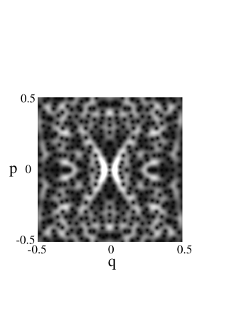
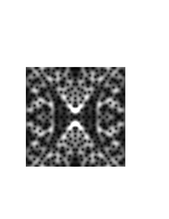
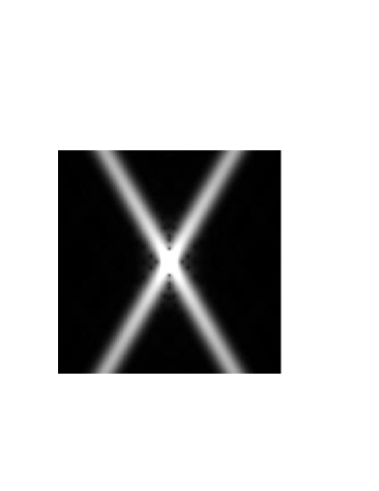
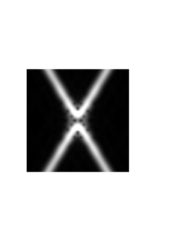
Figure 4: The Husimi functions of some scarred eigenstates of the perturbed cat map. Starting from the left, these have the Hilbert-space dimensions and eigenangles $(N=404,\theta=-1.690)$, $(N=400,\theta=0.050)$, $(N=400,\theta=1.547)$ and $(N=404,\theta=2.995)$. We note that eigenangles are respectively close to $-\pi/2,0,\pi/2$ and $\pi$ and that the states bear a qualitative resemblance to the leading scar function at corresponding values of $\theta$.

We begin by considering some individual wavefunctions. We show in Figure 4 some examples of eigenfunctions of the quantum perturbed cat map which reflect the structure of the leading scar state in Figure 2 at the corresponding eigenangle. The enhancement of the eigenstates along the stable and unstable manifolds as seen here is a well-known characteristic of scarred eigenfunctions. However, the dependence of the detailed pattern of this enhancement on eigenangle and the fact that it can persist into the antiscarred region, is less obvious. Although we do not show examples here, we also expect to find eigenfunctions with enhanced overlaps with subsequent scar states with $i=1,2,\cdots$, whose Husimi functions vary across the spectrum as indicated in Figure 2. The Schnirelman theorem [22] guarantees that such structures cannot dominate individual wavefunctions in the semiclassical limit, However we note that the scar states shrink in phase space as $\hbar\to 0$ and may dominate in a sufficiently small neighbourhood. We also note that even when scar states do not dominate a given wavefunction, locally or otherwise, they should collectively form an efficient basis for calculating and characterising such wavefunctions [20].

Let us now turn to overlap statistics. We have seen that if we use the scar states $|{\chi_{i}(\theta)}\rangle$ as probe states, the statistics of the resulting overlaps

$$y_{i}=\langle{\chi_{i}(\theta)}|{\psi_{n}}\rangle,$$ (20)

should be described by the Gaussian distribution $P(y_{i};\theta)$ given in Eq. (8). Furthermore, overlaps for different values of $i$ should be statistically independent. We now test this supposition using the perturbed cat-map model.

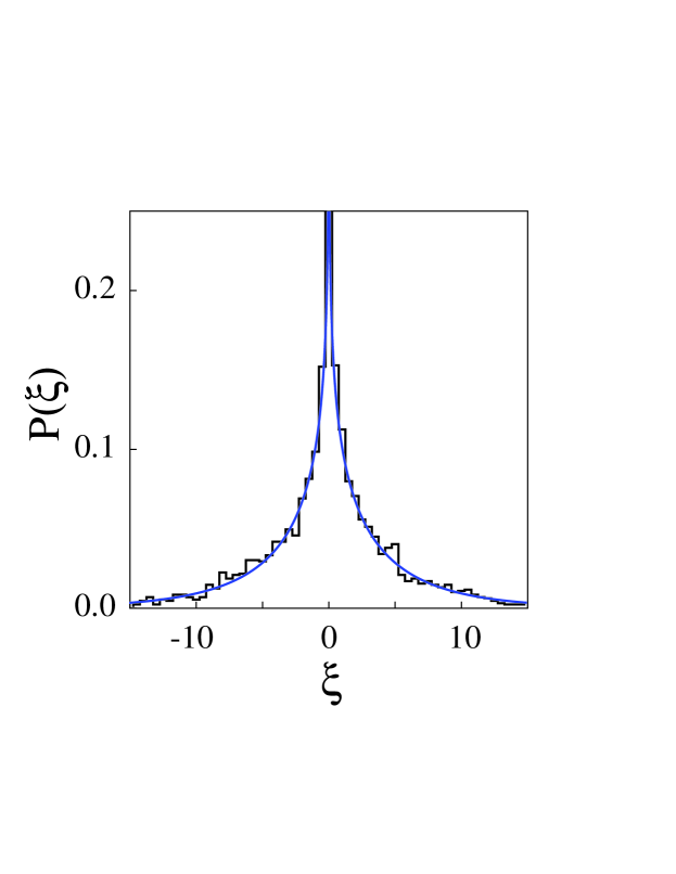
Figure 5: The distribution of $\xi=y_{0}\,y_{1}$, where $y_{i}=\langle{\chi_{i}(0)}|{\psi_{n}}\rangle$. The histogram shows the results of a numerical calculation for a perturbed cat map in which the eigenstates $|{\psi_{n}}\rangle$ in the interval $-0.05\pi<\theta<0.05\pi$ used. The solid line is the theoretical expectation Eq.(21). The symmetry of this result supports the assertion of statistical independence for $y_{0}$ and $y_{1}$.

To verify statistical independence of distinct components $y_{i}$, we consider the variable

$$\xi=y_{i}\,y_{j}\qquad\mbox{with}\quad i\neq j.$$

The distribution for this variable can be calculated as a special case of (6), to give

$$P(\xi;\theta)=\frac{1}{\pi\sqrt{s_{i}(\theta)\,s_{j}(\theta)}}K_{0}\left(\frac{|\xi|}{\sqrt{s_{i}(\theta)\,s_{j}(\theta)}}\right),$$ (21)

where $K_{0}(z)$ is a modified Bessel function. The independence of $y_{i}$ and $y_{j}$ is reflected in the fact that this is an even function of $\xi$. Figure 5 verifies that distribution describes the joint statistics of $y_{0}$ and $y_{1}$ in the case of a perturbed cat map and supports the assertion that these variables are statistically independent. Note that numerical limitations restrict us to relatively modest truncations of the harmonic-oscillator basis in this case — the statistics shown have been computed for scar states with $M=28$ and $\beta=\infty$ — nevertheless the agreement is quite good.

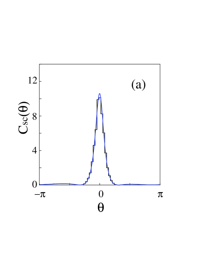
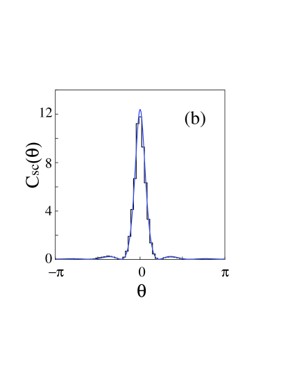
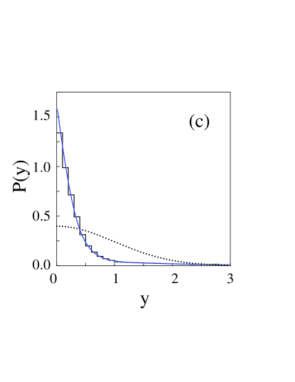
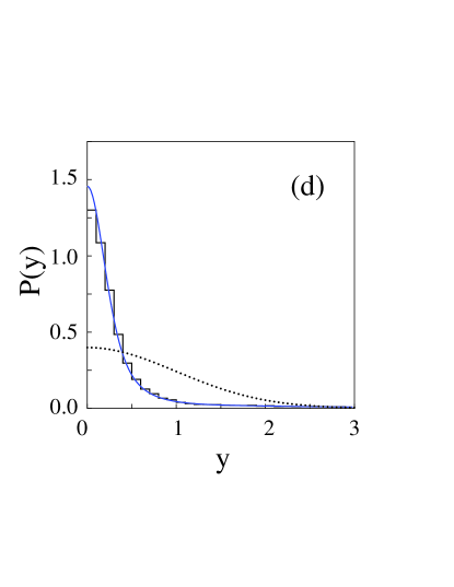
Figure 6: The variance calculated for the scar state $|{\chi_{0}(0)}\rangle$ according to (22) is compared with results for the perturbed cat map as a function of $\theta$. Cases (a) and (b) are respectively for effective truncation dimensions $M=8$ and $M=28$ with $\beta=\infty$ in the scarred region. The accumulated overlap distributions $P(y)$ are shown in (c) and (d), respectively, for the same truncation dimensions. The solid line comes from the present theory and the dotted line is the RMT prediction.

We also consider the statistics of a single component, concentrating on the statistics of $y_{0}$, the overlap with the leading scar state. We first construct the probe state $|{\chi_{0}(0)}\rangle$ for the maximally scarred part of the spectrum and examine its overlap statistics as a function of $\theta$. The variance at any other part of the spectrum is then calculated for this fixed state using

$$C_{\rm sc}(\theta) = \sum_{t}e^{i\theta t}\langle{\chi_{0}(0)}|{\hat{U}_{\rm lin}^{t}}|{\chi_{0}(0)}\rangle.$$ (22)

This is analogous to the envelope for the universal test state considered in [6]. A comparison with numerical results for the perturbed cat map is shown in Figure 6 for two truncation dimensions $M$ of the matrix $\tilde{{\bf C}}(\theta)$. We see that the overlaps are concentrated more in the scarred region and that the height increases as $M$ is increased, consistent with the observation that $s_{0}(0)$ diverges logarithmically with $M$. Note that, as for any fixed state, a spectral average of the variance must average to unity since $\left\langle{C_{\rm sc}}\right\rangle=\langle{\chi_{0}(0)}|{\hat{U}_{\rm lin}^{t=0}}|{\chi_{0}(0)}\rangle=1$. Any growth in the scarred region must therefore be accompanied by a decay elsewhere in the spectrum and this is also visible in Figure 6. This does not contradict the fact that $s_{0}(\theta)$ remains large over the whole spectrum because the leading scar state varies with $\theta$ whereas in this calculation we have used a fixed state $|{\chi_{0}(0)}\rangle$

We also show in Figure 6(c) and (d) the distribution of $y=\langle{\chi_{0}(0)}|{\psi_{n}}\rangle$ about this mean behaviour, averaged over eigenangle $\theta$. The distribution

$$p(y)=\frac{1}{2\pi}\int\,d\theta\,\,p(y;\theta)=\frac{1}{2\pi}\int\,d\theta\frac{1}{\sqrt{2\pi C_{\rm sc}(\theta)}}\,\,e^{y^{2}/2C_{\rm sc}(\theta)},$$ (23)

shown as a solid line describes quite accurately the wavefunction statistics, shown as a histogram. Note the marked difference between these results and the RMT prediction indicated by a dotted line. Similar reults are found for the statistics of $\langle{\chi_{0}(0)}|{\psi_{n}}\rangle$ with $i>0$, although in the deviation from RMT is then less stark.

4 Wavefunction statistics in billiard systems

The discussion so far has been in terms of quantum maps, but we now address the physically more interesting question of time-independent systems, and in particular billiard systems. In this section we describe how the the joint-probability distribution may be applied to such systems, for which an analogy with maps can be made through the boundary-integral formalism. In more generic problems such a connection is made using the transfer-operator formalism of Bogomolny [23].

4.1 Boundary eigenfunctions

We consider eigenfunctions of the Helmholtz equation

$$(\nabla^{2}+k_{n}^{2})\Psi_{n}({\bf x})=0,$$ (24)

satisfying the Dirichlet condition $\Psi_{n}({\bf x})=0$ on the boundary and we assume that the domain is such that the corresponding billiard dynamics is chaotic. In order to apply the results of the preceding sections it is convenient to reformulate this problem in terms of maps, and a natural means of doing this is to use the boundary-integral method, which provides a quantum analog of the classical Poincaré-Birkhoff mapping.

The boundary-integral method has been extensively described elsewhere so here we just describe the key features, primarily to establish notation. For a more detailed description, and in particular for other investigations of scarring in the boundary representations, we refer to [24, 25, 26, 27, 28, 29]. The essential point is that we replace the Helmholtz equation in the interior of the billiard by the integral equation

$$\psi_{n}(s)=\int\,K(s,s^{\prime};k_{n})\psi_{n}(s^{\prime}){\rm d}s^{\prime}$$ (25)

over a coordinate $s$ on the boundary, where

$$\psi_{n}(s)=\left.\frac{\partial\Psi_{n}({\bf x})}{\partial n}\right|_{{\bf x}={\bf x}(s)}$$ (26)

serves as a boundary eigenfunction. The kernel is

$$K(s,s^{\prime};k_{n})=\left.\frac{\partial G({\bf x},{\bf x}(s^{\prime});k_{n})}{\partial n}\right|_{{\bf x}={\bf x}(s)}$$ (27)

where

$$G({\bf x},{\bf x^{\prime}};k_{n})=\frac{i}{2}H_{0}^{(1)}(k_{n}|{\bf x}-{\bf x^{\prime}}|).$$ (28)

is the Green function for the Helmholtz equation.

The integral equation (25) will play the role of a quantum map for us. Even though the map is not unitary [24], we will assert that a straightforward generalisation of the envelope matrix derived in Appendix A constrains the variances of overlaps between harmonic probe states and eigenfunctions. The important point is that iterates of the map concatenate semiclassically in the same way that iterates of a unitary map do and while there are some local modifications of amplitude on classical length scales due to breaking of unitarity, these do not appreciably affect the statistics when phase-space localised probe states are used. In particular, we assert that the statistics of $\psi_{n}(s)$ near a periodic orbit are described by the joint-probability distribution with the structure described in previous sections, at least in the semiclassical limit. In order to write this distribution down we need to define analogues for some of the ingredients we used in the previous sections.

In describing the Poincaré-Birkhoff mapping we use canonical coordinates $(s,v)$ where $s$ is an arc-length coordinate at which a trajectory collides with the boundary and $v=\sin\alpha$, where $\alpha$ is the angle of incidence. We consider wavefunction statistics in the neighbourhood of a point with coordinates $(s_{0},v_{0})$ where a periodic orbit of length $\ell$ intersects the boundary. As a spectral parameter we use $\theta=k\ell-\mu\pi/2$, where $\mu$ is the Maslov index of the periodic orbit — with this definition we will find that that full scarring occurs when $\theta=0\;{\rm mod}\;2\pi$. As probe states we use eigenstates of a harmonic oscillator centred at $(s_{0},v_{0})$ on the boundary section. These are written as boundary wavefunctions of the form

$$\varphi_{l}(s)=\frac{1}{\sqrt{\sigma 2^{l}l!\sqrt{\pi}}}\exp\left[-\frac{(s-s_{0})^{2}}{2\sigma^{2}}+ikv_{0}(s-s_{0})\right]H_{l}\left(\frac{s-s_{0}}{\sigma}\right),$$ (29)

where $H_{l}(z)$ is a Hermite polynomial. As in [7] we let $\sigma$, which provides us with an aspect ratio in phase space of the ellipse defined by the harmonic oscillator, to scale with $k$ as

$$\sigma=\sqrt{\frac{\ell_{0}}{k}}$$

where $\ell_{0}$ is a characteristic length of the billiard. In practice we choose $\ell_{0}$ so that $Q=0$ (that is, so that the invariant manifolds are orthogonal in the corresponding metric). We scale the overlap variables ${\bf x}=(x_{0},x_{1},\cdots)$ as

$$x_{l}\simeq\sqrt{k}\langle{\varphi_{l}}|{\psi_{n}}\rangle=\sqrt{k}\int_{0}^{L}ds\,\,\varphi_{l}^{*}(s)\psi_{n}(s),$$ (30)

where $L$ is the boundary arc length. These scalings are such that the statistics of the components $x_{l}$ do not vary over the spectrum. We also note that $kL$ plays the same role as the dimension $N$ in the case of quantum map.

Figure 7: The cardioid billiard and the periodic orbit used in numerical calculation.

For numerical purposes we consider the cardioid billiard, which is defined in polar coordinates by

$$r=1+\cos\theta.$$ (31)

We consider just the odd-parity states and therefore restrict ourselves to the half-cardioid illustrated in Figure 7. For simplicity we treat the shortest periodic orbit, also shown in Figure 7, which has stability exponent $\rho\simeq 0.693$ and length $\ell=3\sqrt{3}/2$. We examine wavefunction statistics where this intersects the boundary section at $s_{0}\simeq 2.00$ and $v_{0}=0$.

Figure 8: The overlap probabilities $y_{n}^{2}=k|\langle{\chi_{0}}|{\psi_{n}}\rangle|^{2}$ for the leading scar state are shown as a function of $k$. In (a) the state $\chi_{0}$ is constructed for the scarred part of the spectrum with $\theta=0$ and in (b) it is constructed for the antiscarred part, with $\theta=\pi$. In each case the scar state has been calculated using a truncation dimension of $M=12$.

We calculate scar states as described in the previous sections, with the obvious modifications appropriate to billiards, and denote the corresponding boundary functions by $\chi_{i}(s;\theta)$. Let us begin by considering the overlap probability

$$y_{n}^{2}=k|\langle{\chi_{0}(0)}|{\psi_{n}}\rangle|^{2},$$ (32)

for the leading scar state calculated for the scarred part of the spectrum. The scaling with $k$ here is designed so that the average value does not change across the spectrum. This overlap probability is calculated for individual eigenfunctions and the results shown in Figure 8(a) as a function of $k$. As expected we find strong peaks in typical values localised around values of $k$ for which $\theta=k\ell-\mu\pi/2=0\;{\rm mod}\;2\pi$, with a compensating suppression between peaks. The sharp contrast between the peaks and valleys in this figure is a reflection of the extent to which $\chi_{0}(s;0)$ maximises the deviation of statistics from RMT. We also show, in Figure 8(b) the overlap probabilities for the leading scar state $\chi_{0}(s;\pi)$ constructed for the antiscarred part of the spectrum where $\theta=\pi\;{\rm mod}\ 2\pi$. Once again we find periodic peaks in the average value of the overlap probability, albeit with a somewhat reduced contrast. Note also, however, that the peaks in Figure 8(b) occur when there are troughs in Figure 8(a) and vice versa. In other words, we have defined a probe state for which significantly larger than average overlaps occur in parts of the spectrum which are normally associated with antiscarring. Although we do not show them explicitly, each of these sequences can be defined also for subsequent scar states $\chi_{i}(s;\theta)$ with $i>0$; these subsequent sequences peak in the same parts of the spectrum but are statistically independent.

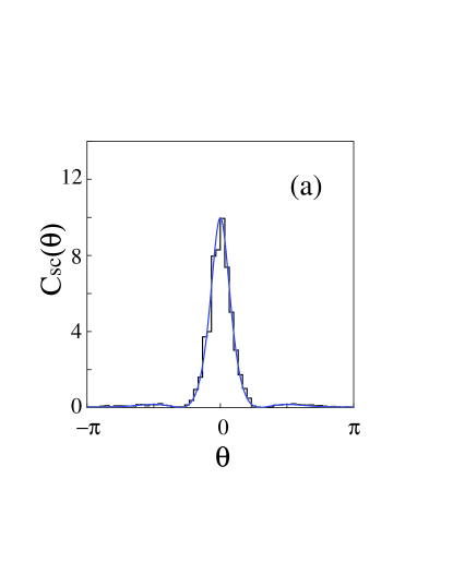
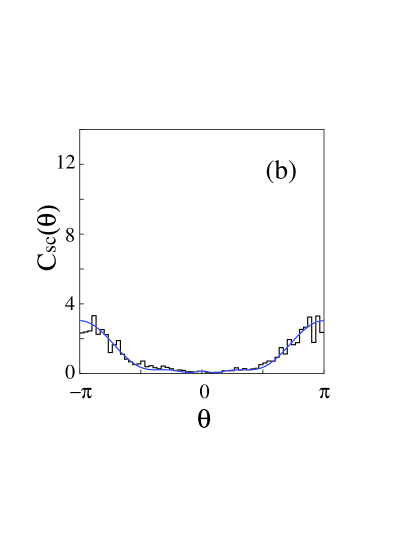
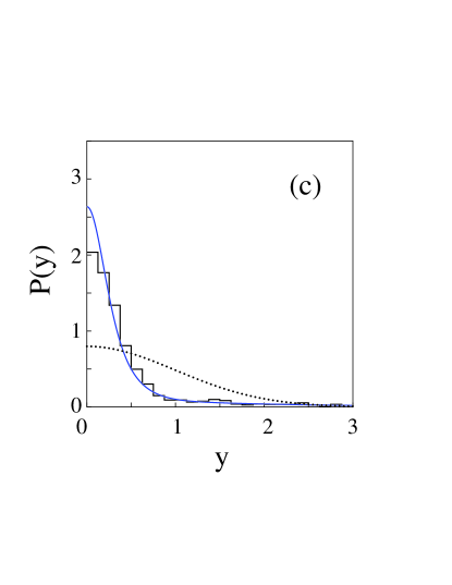
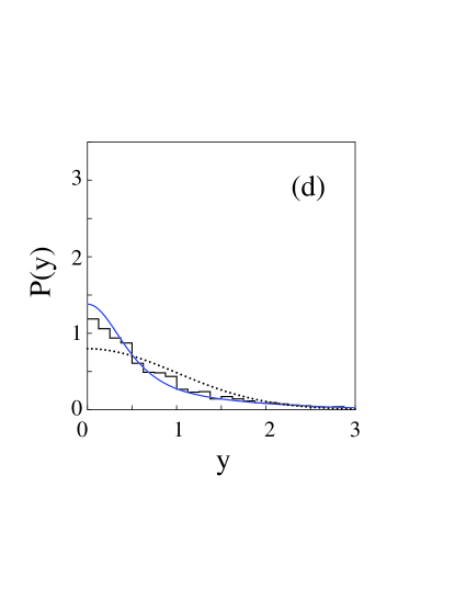
Figure 9: The partial variance $\left\langle{y^{2}}\right\rangle$ is shown as a function of $\theta$. In (a) and (b) we respectively show results for the scar state of the scarred region ($y^{2}=k|\langle{\chi_{0}(0)}|{\psi_{n}}\rangle|^{2}$) and of the antiscarred region ($y^{2}=k|\langle{\chi_{0}(\pi)}|{\psi_{n}}\rangle|^{2}$). The solid lines show the envelope functions $C_{{\rm sc},0}(\theta)$ and $C_{{\rm sc},\pi}(\theta)$ calculated in analogy with (22). In (c) and (d) we show the corresponding accumulated overlap distributions $P(y)$ describing the distribution of individual overlaps about the averages depicted in (a) and (b). The solid line comes from the present theory and the dotted line is the RMT prediction. That is, in (c) we compare a histogram of $y=k|\langle{\chi_{0}(0)}|{\psi_{n}}\rangle|$ with theory and in (d) we do the same for $y=k|\langle{\chi_{0}(\pi)}|{\psi_{n}}\rangle|$.

To make a more quantitative comparison with the theory of the scar state we collate the overlap probabilities as a function of $\theta$ and compare with the prediction of (22) (and its generalisation to the antiscarred region) in Figures 9(a) and (b). These describe envelopes for Figure 8 and confirm that the detailed predictions for the variances using the envelop matrix ${\bf C}(\theta)$ work quantitatively in this billiard system. A comparison of the statistics of the distribution of individual states about this average in (c) and (d) also supports the hypothesis of Gaussian statistics in this context. Calculations of correlation and the statistics of higher scar states work similarly to the case of quantum maps, as investigated in the previous section, and we do not give further numerical details in the boundary representation here. Instead we turn to a discussion of how we may formulate these statistical properties in terms of full wavefunctions in the interior of the billiard.

4.2 Full eigenfunctions

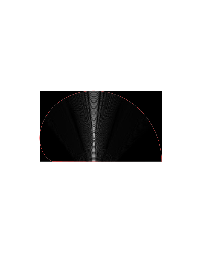
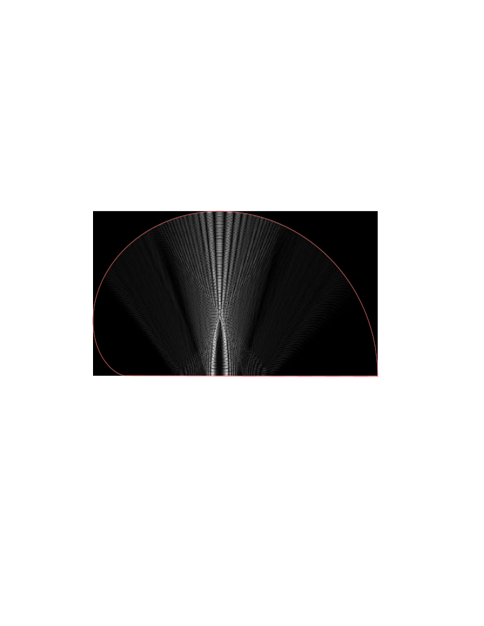
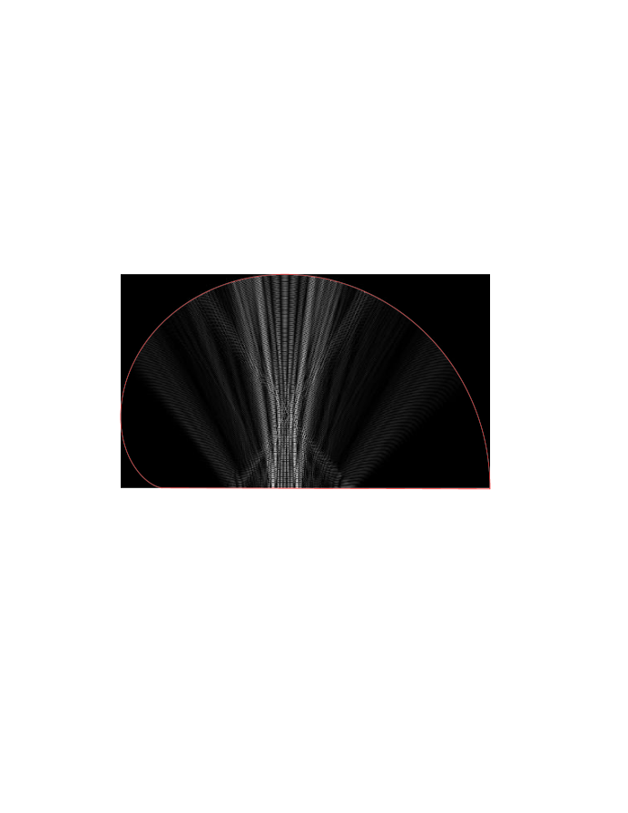
Figure 10: Examples of leading scarfunctions $\Phi_{0}^{scar}({\bf x};k)$ calculated for (clockwise from top left) $k=999.40$, $998.80$, $1000.01$ and $1000.61$. These correspond respectively to $\theta=0$, $\pi/2$, $\pi$ and $3\pi/2$.

The scar states for billiards have so far been given in the boundary-integral formalism. We now propose corresponding probe states which are appropriate to full wavefunctions in the interior of the billiard. Given an eigenfunction $\psi_{n}(s)$ of the boundary-integral equation, the full eigenfunction $\Psi_{n}(x)$ is obtained from it using Green’s identity, giving

$$\Psi_{n}({\bf x})=\frac{1}{2}\int G({\bf x},{\bf x}(s^{\prime});k_{n})\,\psi_{n}(s^{\prime})\,{\rm d}s^{\prime}.$$ (33)

We define probe states in the interior of the billiard in analogy with this equation. That is, given a probe state $\varphi(s)$ in the boundary representation, whether it be a harmonic-oscillator eigenstate, a scar state or otherwise, we define a corresponding probe state in the interior using

$$\Phi({\bf x})=\frac{1}{2}\int G({\bf x},{\bf x}(s^{\prime});k_{n})\,\varphi(s^{\prime})\,{\rm d}s^{\prime}.$$ (34)

This function automatically satisfies the Helmholtz equation in the interior but, because $\varphi(s)$ does not satisfy the boundary integral equation, does not satisfy the Dirichlet boundary conditions placed on $\Psi_{n}({\bf x})$. Nevertheless it provides a perfectly well defined function in the interior of the billiard and we may use it to characterise the wavefunction near the periodic orbit.

We provide an argument in Appendix B which indicates that, given a probe state which is localised in phase space around a point $(s_{0},v_{0})$, then the boundary overlap $\langle{\varphi}|{\psi_{n}}\rangle$ and the full overlap $\langle{\Phi}|{\Psi_{n}}\rangle$ approximately coincide,

$$\langle{\Phi}|{\Psi_{n}}\rangle\simeq g(s_{0},p_{0})\langle{\varphi}|{\psi_{n}}\rangle,$$ (35)

up to a geometrical factor $g(s_{0},p_{0})$ which depends on the location the probe state in phase space but is independent of $\psi_{n}$. Following appropriate normalisation, the predictions for the statistics of the boundary overlaps may therefore be carried over to the overlaps defined in the interior.

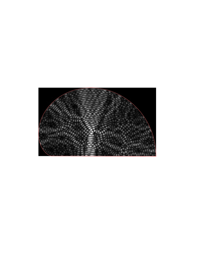
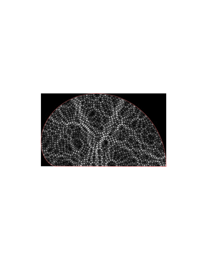
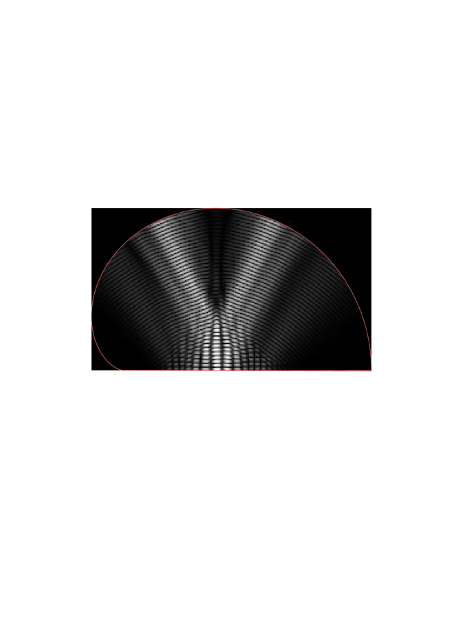
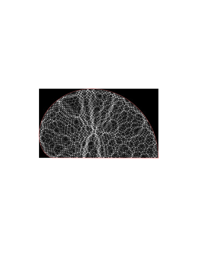
Figure 11: At left we show scarred eigenfunctions with, from top to bottom, $k_{n}=92.54$, $107.48$ and $118.66$. These correspond respectively to $\theta$ near $0$ (in the scarred region), $-\pi/2$ and $\pi/2$. These may be compared with the corresponding scarfunctions $\Phi_{0}^{scar}({\bf x};k_{n})$, shown on the right. The overlap probabilities are respectively $38.2$, $21.0$ and $21.5$ times larger than the RMT average. Details of the scar state can readily be detected in the eigenfunction in the scarred region. Although the correspondence is less obvious for the other eigenfunctions, features such as numbers and positions of nodes of the scarfunction can sometimes be seen in the eigenfunctions.

In particular, we may conclude that in a given part of the spectrum the interior functions constructed from the leading boundary scar states $\chi_{i}(s;\theta)$, $i=0,1,2,\cdots$, should have especially large overlaps with the billiard eigenfunctions. Let us denote by $\Phi_{i}^{scar}({\bf x};k)$ the interior function obtained from a boundary scar state $\chi_{i}(s;\theta)$. We show examples of these interior functions in Figure 10 corresponding to values $\theta=0$, $\pi/2$, $\pi$ and $3\pi/2$ of the spectral parameter $\theta$ and $k$ near $1000$. We remark that these states are somewhat extended spatially around the periodic orbit in configuration space, a reflection of the fact that phase space representations of the scar states extend quite far along the stable and unstable manifolds. We also remark that, near intersections of the periodic orbit with the boundary, these scarfunctions approximately satisfy the Dirichlet boundary conditions placed on the full solution. This is a reflection of the fact that they are derived from boundary states which are approximate eigensolutions of the boundary integral operator sufficiently near the periodic orbit in phase space.

These functions provide us with templates for the behaviour of heavily scarred eigenfunctions near periodic orbits in different parts of the spectrum. We compare in Figure 11 some cases of individual scarred eigenfunctions with the corresponding leading scarfunction $\Phi_{0}^{scar}({\bf x};k_{n})$. In some cases, such as the eigenfunction with $k_{n}=92.54$, one can identify characteristics of the corresponding scarfunction (such as the number of nodes seen along a periodic orbit). In other scarred eigenfunctions, especially those in the antiscarred region where the corresponding scarfunctions are not well-localised, a detailed correspondence is less evident visually, although there is nevertheless a large overlap with the appropriate $\Phi_{0}^{scar}({\bf x};k_{n})$. We emphasise that, although not shown explicitly here, for each $k_{n}$ these interior functions are the leading members of a sequence $\Phi_{i}^{scar}({\bf x};k_{n})$, $i=0,1,2,\cdots$ and each of these functions will tend to have especially large overlaps with $\psi_{n}$.

By tracking the scar states as a function of $\theta=k\ell-\mu\pi/2$ we thus define continuous families of interior functions which approximately vanish on the boundary near bounces of the periodic orbit. While our notation suggests boundary functions $\chi_{i}(s;\theta)$ which are $2\pi$-periodic in $\theta$, we should note that as we increase $\theta=k\ell-\mu\pi/2$ by $2\pi$, the effective value of $\hbar$ decreases and there is a slow modulation of $\chi_{i}(s;\theta)$ with $k$. (While the coefficients of $\chi_{i}(s;\theta)$ in a basis of the harmonic states $\varphi_{l}(s)$ defined in (29) are asymptotically periodic in $\theta$ as $M\to\infty$, the states $\varphi_{l}(s)$ themselves shrink as $k$ increases). To emphasise this evolution, we label the interior functions $\Phi_{i}^{scar}({\bf x};k)$ with $k$ rather than $\theta$. As $k$ increases by $2\pi/\ell$ the form of $\Phi_{i}^{scar}({\bf x};k)$ transverse to the periodic orbit is approximately periodic but an extra node appears in the longitudinal direction. Over many such quasiperiods, there is a gradual shrinkage in the transverse length scale and an increase in the number of nodes along the orbit. Throughout this evolution, $\Phi_{i}^{scar}({\bf x};k)$ exactly satisfies the Helmholtz equation and approximately satisfies the Dirichlet boundary conditions near the periodic orbit.

We remark finally that although we do not show so explicitly here, these considerations should also allow us to characterise scarring in general time-dependent systems. Starting with a formal representation of eigenstates on a Poincaré section as in the Bogomolny transfer method, we can define an analogous extension of probe states from the section to the full space and therefore provide statistical predictions for overlap statistics which can be calculated concretely from the full wave function.

5 Conclusion

We have shown that the joint-probability distribution $P({\bf x};\theta)$ describing wavefunction statistics in a harmonic-oscillator basis near a periodic orbit leads to the definition of a set of probe states which describe in a natural way the morphology of scarring in a given part of the spectrum. That is, in a given part of the spectrum (parametrised by $\theta$), we define a set of probe states $|{\chi_{i}(\theta)}\rangle$ with $i=0,1,\cdots$ such that the overlaps $\langle{\chi_{i}(\theta)}|{\psi_{n}}\rangle$ are expected to be especially large, on average, and statistically independent. In particular these probe states offer a template for the structure of scarred wavefunctions and tell us how the shape of scarring changes across the spectrum.

The scar states, in offering a basis set for which we expect enhanced overlap with chaotic eigenfunctions, may in particular prove useful in explicit computation as outlined in [14]. We note also the fact that we can obtain such enhanced overlap probabilities in parts of the spectrum normally associated with antiscarring, where we expect a suppression of overlap with a Gaussian basis state on the periodic orbit. We have illustrated our results with explicit calculation for a quantum map model and have also outlined briefly how these ideas may be applied to billiard systems.

Acknowledgements
This paper is supported by the EPSRC under the Fast Stream scheme.

Appendix A Appendix: The matrix elements of the linear evolution operator

We here give explicit formulas for the calculation of the the linear correlation matrix ${\bf A}(t)$ in a harmonic oscillator basis. A detailed derivation of these results has been given in [17] and here we state the key features.

To begin we characterise linear classical evolution near a periodic orbit using the stability exponent $\rho$ and the parameter $Q$ described in the main text. We then define angles $\psi(t)$ and $\varphi(t)$ using

$$\cosh\rho t+iQ\sinh\rho t=\sec\psi(t)\,e^{i\varphi(t)},$$ (36)

and we choose these angles to lie in the ranges $0<\psi(t)<\pi/2$ and $-\psi(t)<\varphi(t)<\psi(t)$ respectively.

Then we may calculate the matrix elements $A_{lk}(t)$ for $l=k+2n$ and $n\geq 0$ using the polar form

$$A_{k+2n,k}(t)=G_{kn}(\psi(t))\;e^{i(k+1/2)(\varphi(t)-\mu t\pi)+in\varphi(t)+in\pi/2},$$ (37)

where $\mu$ is the Maslov index of the periodic orbit concerned and the amplitude is

$$G_{kn}(\psi)=\sqrt{\frac{k!}{(k+2n)!}}\;\frac{(2n)!}{2^{n}n!}\;\;\sin^{n}\psi\,\sqrt{\cos\psi}\;C_{k}^{n+1/2}(\cos\psi),$$

where $C_{k}^{\alpha}(x)$ denotes a Gegenbauer polynomial. We assume $n\geq 0$ and $t>0$ in (37) and use $A_{lk}^{*}(-t)=A_{lk}(t)=A_{kl}(t)$ to calculate the correlation function when $t<0$ or $l<k$. We note finally that $A_{kl}(t)=0$ if $k$ and $l$ do not have the same parity.

Appendix B Appendix: interior and boundary overlaps

In this appendix we show that if a boundary probe function $\varphi(s)$ is appropriately localised near a point $(s_{0},v_{0})$ in phase space then there is a relationship of the form given in (35) between the boundary overlap $\langle{\varphi}|{\psi_{n}}\rangle$ the full overlap $\langle{\Phi}|{\Psi_{n}}\rangle$ of the corresponding interior functions, defined by (33) and (34). Substituting these defining relations into the interior integral for $\langle{\Phi}|{\Psi_{n}}\rangle$ we find

$$\langle{\Phi}|{\Psi_{n}}\rangle=\int_{0}^{L}{\rm d}s\int_{0}^{L}{\rm d}s^{\prime}\;f(s,s^{\prime})\,\varphi^{*}(s)\psi_{n}(s^{\prime}),$$ (38)

where

$$f(s,s^{\prime})=\frac{1}{4}\int_{D}\,G^{*}({\bf x},{\bf x}(s);k)\,G({\bf x},{\bf x}(s^{\prime});k)\,{\rm d}{\bf x}$$ (39)

and $D$ denotes the billiard domain. We consider in particular the case where the probe state is of the form $\varphi(s)=e^{ikv_{0}s}h(s)$ where we suppose that $h(s)$ is supported in a neighbourhood of $s_{0}$ that is small in comparison with the length scales of the billiard but varies on a scale longer than the length scale $1/k$ typical of wavefunctions. This is the case for example for the basis probe states $\varphi_{l}(s)$, which vary and decay on a length scale of order $1/\sqrt{k}$. It is also the case for any finite combination of them such as the truncated scar states we use. We claim that $f(s,s^{\prime})$ then behaves essentially as a delta-function when integrated against $\varphi(s)$, giving

$$\int\varphi^{*}(s)f(s,s^{\prime}){\rm d}s\simeq g(s^{\prime},v_{0})\varphi^{*}(s^{\prime})$$

where $g(s^{\prime},v_{0})$ is determined from the geometry of the billiard and varies with $s^{\prime}$ on a classical length scale. Since $\varphi(s)$ is localised to a neighbourhood of a point $s_{0}$ that is smaller than classical length scales then we may further replace $g(s^{\prime},v_{0})$ by $g(s_{0},v_{0})$ in the overlap integral and approximate

$$\langle{\Phi}|{\Psi_{n}}\rangle\simeq g(s_{0},v_{0})\langle{\varphi}|{\psi_{n}}\rangle.$$

The overlaps $\langle{\Phi}|{\Psi_{n}}\rangle$ and $\langle{\varphi}|{\psi_{n}}\rangle$ then coincide up to a factor which depends on the position in phase space of the probe state but is independent of $\psi_{n}$. This means in particular that predictions for the statistics of $\langle{\varphi}|{\psi_{n}}\rangle$ carry over to $\langle{\Phi}|{\Psi_{n}}\rangle$ after appropriate normalisation.

We justify this assertion by using the asymptotic representation of the Hankel function

$$H_{0}^{(1)}(k|{\bf x}-{\bf x}(s)|)\simeq\sqrt{\frac{2}{\pi k|{\bf x}-{\bf x}(s)|}}e^{ik|{\bf x}-{\bf x}(s)|-i\pi/4}$$

for the Green functions in the integral (39), giving

$$f(s,s^{\prime})\simeq\frac{1}{8\pi k}\int_{D}\frac{e^{ik(|{\bf x}-{\bf x}(s^{\prime})|-|{\bf x}-{\bf x}(s)|)}}{\sqrt{|{\bf x}-{\bf x}(s)||{\bf x}-{\bf x}(s^{\prime})|}}\;{\rm d}{\bf x}.$$ (40)

Fixing $s$ and $s^{\prime}$ temporarily, we are free to choose the origin of coordinates to be the midpoint between ${\bf x}(s)$ and ${\bf x}(s^{\prime})$, so that ${\bf x}(s)={\bf a}/2$ and ${\bf x}(s^{\prime})=-{\bf a}/2$. For large $k$ the rapid oscillation in the integrand when $s$ and $s^{\prime}$ are distinct means that $f(s,s^{\prime})$ is peaked around $s\approx s^{\prime}$. To evaluate the integral near this peak, we consider contributions from points for which $r=|{\bf x}|\gg a=s-s^{\prime}$. We then approximate the phase of the integrand by

$$k\left(|{\bf x}-{\bf x}(s^{\prime})|-|{\bf x}-{\bf x}(s)|\right)=ka\sin\theta+O\left(\frac{ka^{3}}{r^{2}}\right),$$

where $(r,\theta)$ are polar coordinates for ${\bf x}$ relative the midpoint of ${\bf x}(s)$ and ${\bf x}(s^{\prime})$, which we approximate as lying on the boundary, and the normal to the boundary there. This substitution for the phase is valid as long as $a\ll(R^{2}/k)^{1/3}$, where $R$ is the length scale of the billiard. We then approximate the integral in (40) by

$$f(s,s^{\prime}) \simeq \frac{1}{8\pi k}\int_{D}\frac{e^{ika\sin\theta}}{r}\;r{\rm d}r{\rm d}\theta$$

$$= \frac{1}{8\pi k}\int_{-\pi/2}^{\pi/2}e^{ika\sin\theta}L(\theta)\,{\rm d}\theta$$

where $L(\theta)$ is the length inside the billiard of a line passing through the origin at polar angle $\theta$. For convex billiards, $r=L(\theta)$ simply defines the shape of the boundary in polar coordinates.

As a function of $(s,s^{\prime})$, this integral is effectively supported on a length scale $1/k$ near $s\approx s^{\prime}$ or $a\approx 0$. When integrated against a probe state which varies over a longer scale such as $1/\sqrt{k}$, we may therefore treat it as a $\delta$-like pulse. In fact, we may approximate

$$\int\varphi^{*}(s)f(s,s^{\prime}){\rm d}s = \int h^{*}(s)e^{-ikv_{0}s}f(s,s^{\prime})\,{\rm d}s$$

$$\simeq \frac{1}{8\pi k}e^{-ikv_{0}s^{\prime}}h^{*}(s^{\prime})\int_{-\infty}^{\infty}\left[\int_{-\pi/2}^{\pi/2}e^{ika(\sin\theta-v_{0})}L(\theta)\,{\rm d}\theta\right]{\rm d}a$$

$$\simeq \frac{1}{8\pi k}\varphi^{*}(s^{\prime})\int_{-\pi/2}^{\pi/2}\left[\int_{-\infty}^{\infty}e^{ika(\sin\theta-v_{0})}{\rm d}a\right]L(\theta)\,{\rm d}\theta$$

$$\simeq \frac{1}{8\pi k}\varphi^{*}(s^{\prime})\int_{-\pi/2}^{\pi/2}\left[2\pi\delta(k\left(\sin\theta-v_{0})\right)\right]L(\theta)\,{\rm d}\theta$$

$$= \frac{1}{4k^{2}\cos\theta_{0}}L(\theta_{0})\varphi^{*}(s^{\prime}),$$

where $v_{0}=\sin\theta_{0}$. Here, $L(\theta_{0})$ is the length of a chord which leaves the point $s^{\prime}$ at an angle $\theta_{0}$ to the normal. It depends on $s^{\prime}$ and we therefore replace $L(\theta_{0})$ by $L(s^{\prime},\theta_{0})$ in our notation to emphasise that it changes as we change the centre $s\approx s^{\prime}$ of the peaked function $f(s,s^{\prime})$.

If $h(s)$ is sufficiently slowly varying we may therefore approximate the expression for the inner product (38) by

$$\langle{\Phi}|{\Psi_{n}}\rangle\simeq\frac{1}{4k^{2}\cos\theta_{0}}\int_{0}^{L}L(s^{\prime},\theta_{0})\varphi^{*}(s^{\prime})\psi_{n}(s^{\prime})\,{\rm d}s^{\prime}.$$

If, however, $h(s)$ is at the same time sufficiently localised around $s_{0}$, then we can replace this in turn by

$$\langle{\Phi}|{\Psi_{n}}\rangle\simeq\frac{L(s_{0},\theta_{0})}{4k^{2}\cos\theta_{0}}\int_{0}^{L}\varphi^{*}(s^{\prime})\psi_{n}(s^{\prime})\,{\rm d}s^{\prime}=\frac{L(s_{0},\theta_{0})}{4k^{2}\cos\theta_{0}}\,\langle{\varphi}|{\psi_{n}}\rangle$$

This verifies our assertion that $\langle{\Phi}|{\Psi_{n}}\rangle$ and $\langle{\varphi}|{\psi_{n}}\rangle$ approximately coincide up to a geometrical factor

$$g(s_{0},v_{0})=\frac{L(s_{0},\theta_{0})}{4k^{2}\cos\theta_{0}}$$

which depends on $k$ and the location of the probe function $\varphi(s)$ but is independent of $\psi_{n}(s)$.

It should be noted that for scarring around a general periodic orbit we will need to consider probe functions which are localised not around a single point $(s_{0},v_{0})$ on the boundary section but around a series of points $(s_{t},v_{t})$, $t=0,1,\cdots,T$ representing the bounces of a periodic orbit on the boundary. In this case we consider probe states of the form $\varphi(s)=\sum_{t}\varphi_{t}(s)$ where each component is localised in the section around a single point $(s_{t},v_{t})$. The interior overlap $\langle{\Phi}|{\Psi_{n}}\rangle$ is then a sum of terms of the form given above, each with a geometrical factor $g(s_{t},v_{t})$ which depends on the the angle of incidence of the periodic orbit at the corresponding bounce and the length of the orbit segment to the next bounce. We can recover a simple scaling such as given in (35) if we scale each of the components $\varphi_{t}$ of $\varphi$ by the corresponding geometrical factor before computing the overlap (or alternatively by redefining the boundary inner product). A detailed treatment of this procedure will presumably lead to a formulation in which the boundary integral operator is replaced, semiclassically at least, by a unitary evolution (see [24], but do not pursue that option here. Instead we note that our explicit calculations have been for a two-bounce orbit normally incident on the boundary and in that case the geometrical factor is the same for both bounces and no such adjustment is necessary.

References

- [1] O. Bohigas, M. J. Gianonni and C. Schmidt, Phys. Rev. Lett. 52, 1 (1984).
- [2] Baowen Li and M. Robnik, J. Phys. A 27. 5509 (1994).
- [3] E. E. Narimanov et al, Phys. Rev. B 64, 235329 (2001).
- [4] L. Kaplan, Phys. Rev. E 62, 3476 (2000).
- [5] L. Kaplan, Phys. Rev. Lett. 80, 2582 (1998).
- [6] L. Kaplan and E. J. Heller, Ann. Phys. 264, 171 (1998); L. Kaplan and E. J. Heller, Phys. Rev. E 59, 6609 (1999); L. Kaplan, Nonlinearity 12, R1 (1999).
- [7] W. E. Bies, L. Kaplan, M. R. Haggerty, E. J. Heller, Phys. Rev. E 63, 66214 (2001).
- [8] S. W. McDonald, Ph.D. thesis, University of California at Berkeley, Lawrence Berkeley Laboratory Report No. 14837, 1983; S. W. McDonald and A. N. Kaufman, Phys. Rev. A 37, 3067 (1988).
- [9] E. J. Heller, Phys. Rev. Lett. 53, 1515 (1984).
- [10] E. B. Bogomolny, Physica D 31, 169 (1988).
- [11] M. V. Berry, Proc. R. Soc. Lond. A 423,219 (1989).
- [12] G. G. de Polavieja, F. Borondo and R. M. Benito, Phys. Rev. Lett. 73, 1613 (1994).
- [13] S. Nonnenmacher and A. Voros, J. Phys. A 30, 295 (1997).
- [14] E. G. Vergini and G. G. Carlo, J. Phys. A: Math. Gen. 34, 4525 (2001); E. G. Vergini and G. G. Carlo, J. Phys. A: Math. Gen. 38, 7965 (2001).
- [15] D. A. Wisniacki et al, Phys. Rev. E, 63 066220 (2001).
- [16] F. Faure, S. Nonnenmacher and S. de Bièvre, arXiv:nlin.CD/0207060.
- [17] S. C. Creagh, S.-Y. Lee, and N. D. Whelan, Ann. Phys. 295, 194 (2002)
- [18] T. M. Antonsen, E. Ott, Q. Chen, and R. N. Oerter, Phys. Rev. E 51, 111 (1995).
- [19] It should also be noted that the divergence of these overlaps is relative to the expectation for an overlap with a generic state. We normalise our states, in the case of a quantum map on a Hilbert space of dimensions , so that , whereas at worst we expect the overlap probability with an appropriate test state to diverge logarithmically with (as determined by the maximum value of for which localised propagation defining is sensible). In particular there is no violation of Schnirelman [22].
- [20] E. G. Vergini, J. Phys. A: Math. Gen. 33, 4709 (2000); E. G. Vergini and G. G. Carlo, J. Phys. A: Math. Gen. 33, 4717 (2000)
- [21] A. M. F. Rivas and A. M. Ozorio de Almeida, Nonlinearity 15, 681 (2002).
- [22] A. I. Schnirelman, Usp. Mat. Nauk. 29, 181 (1974); A. I Schnirelman, in V. F. Lazutkin KAM Theory and Semiclassical Approximations to Eigenfunctions (Springer, 1993).
- [23] E. B. Bogomolny, Nonlinearity 5, 805 (1992).
- [24] P. A. Boasman, Ph. D thesis, University of Bristol, (1992).
- [25] T. Prosen, Physica D 91, 244 (1996).
- [26] J.-M. Tualle and A. Voros, Chaos, Soliotns and Fractals 5, 1085 (1995).
- [27] D. Klakow and U. Smilanski, J. Phys. A 29, 3213 (1996).
- [28] F. P. Simonotti, E. Vergini and M. Saraceno, Phys. Rev. E 56 3859 (1997).
- [29] A. Bäcker et al, arXiv:nlin.CD/0207034.