Heteroclinic Contours in Neural Ensembles and the Winnerless Competition Principle

Abstract

The ability of nonlinear dynamical systems to process incoming information is a key problem of many fundamental and applied sciences. Information processing by computation with attractors (steady states, limit cycles and strange attractors) has been a subject of many publications. In this paper we discuss a new direction in information dynamics based on neurophysiological experiments that can be applied for the explanation and prediction of many phenomena in living biological systems and for the design of new paradigms in neural computation. This new concept is the Winnerless Competition (WLC) principle. The main point of this principle is the transformation of the incoming identity or spatial inputs into identity-temporal output based on the intrinsic switching dynamics of the neural system. In the presence of stimuli the sequence of the switching, whose geometrical image in the phase space is a heteroclinic contour, uniquely depends on the incoming information. The key problem in the realization of the WLC principle is the robustness against noise and, simultaneously, the sensitivity of the switching to the incoming input. In this paper we prove two theorems about the stability of the sequential switching and give several examples of WLC networks that illustrate the coexistence of sensitivity and robustness.

Paper in press for ’International Journal of Bifurcation and Chaos’ (2004), Vol. 14 (4).

1 Introduction

Computing with a dynamical system implies that this system changes its behavior depending on the quality and quantity of the incoming information. This is an enormous field and we will concentrate here only on the concept of Winnerless Competition (WLC) that, as we think, is a general principle for information processing by dynamical systems.

Information processing with WLC dynamics is a new area for theoretical study. However, WLC itself has already been observed in many well known experiments in hydrodynamics [Busse & Heikes, 1980], population biology [May & Leonard, 1975] and laser dynamics [Roy, 1999]. For example, the convective roll patterns in a rotating plane layer demonstrate a sequential changing of direction as a result of the competition between different roll orientations (when the rotation rate is large enough, e.g. Kuppers-Lortz instability [Küppers & Lortz, 1969]). For a large Prandtle number the critical angle is close to $60^{o}$ (for the steady state rolls it is $120^{o}$). Due to the appearance of new rolls that are also unstable, no pattern becomes a winner and, as a result of the competition, they switch sequentially. Small non-Boussinesq effects are able to make such sequence periodic [Rabinovich et al., 2000a].

The discussed process can be described by Lottka-Volterra equations that are well known in population biology and can explain the competition between three spices [May & Leonard, 1975]:

$$\dot{a}_{1} = a_{1}[1-(a_{1}+\rho_{12}a_{2}+\rho_{13}a_{3})]$$

$$\dot{a}_{2} = a_{2}[1-(a_{2}+\rho_{21}a_{1}+\rho_{23}a_{3})]$$

$$\dot{a}_{3} = a_{3}[1-(a_{3}+\rho_{31}a_{1}+\rho_{32}a_{3})]$$

In biology the variable $a_{i}(t)$ is the number of individuals in the $i$–th population at time $t$, and $\rho_{ij}$ are competition coefficients measuring the extent to which the $j$th species affects the growth rate of the $i$–th species. In convection, the variables $a_{i}$ are the intensities of the competitive modes: $a_{i}=|c_{i}|^{2}$, and we suppose that the vertical component of the velocity field is (in the limit of small amplitudes) $u_{x}=f(z)\sum_{j=1}^{3}c_{j}(t)exp\{i{\bf k}_{j}\cdot\bf{r}\}$, where $z$ is the component of the position vector ${\bf r}$ in the vertical direction and ${\bf k}_{j}$ are the wave vectors [Busse & Heikes, 1980, Rabinovich et al., 2000a].

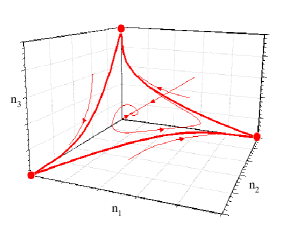
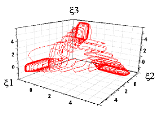
Figure 1: Left panel: phase protrait corresponding to the autonomous WLC dynamics of a three-dimensional case. Right panel: projection of a nine-dimensional heteroclinic orbit of three inhibitory coupled FitzHugh-Nagumo spiking neurons in a three dimensional space (the variables $\xi_{1}$, $\xi_{3}$, $\xi_{3}$ are linear combinations of the actual phase variables of the system [Rabinovich et al., 2000b]) –see also Sec. 5.1–.

The non-symmetry of the coefficients $\rho_{ij}$, for example $\rho_{12}=\rho_{23}=\rho_{31}\equiv\rho_{+}>1$, $\rho_{21}=\rho_{32}=\rho_{13}\equiv\rho_{-}<1$, guarantees the WLC behavior of the discussed dynamical system. The mathematical image of such behavior is a heteroclinic contour in the phase space $a_{1}(t)$, $a_{2}(t)$, $a_{3}(t)$ (see Fig. 1). Results related to symmetric cases have been reporter earlier [Ashwin and Field, 1999] and [Ashwin and Chossat, 1998].

The questions that we are going to discuss below are: (i) what are the conditions for the robustness of the WLC, i.e. the topological similarity of the perturbed and original heteroclinic contour; and (ii) how subsystems with WLC behavior interact with each other.

The paper is organized in the following way. First we describe a class of models that use the WLC principle for the representation and processing of incoming information (Sec. 2). Then we discuss the existence and stability of the heteroclinic contour (Sec. 3), and the robustness, i.e. birth of a stable limit cycle in the vicinity of the destroyed heteroclinic loop in a perturbed system (Sec. 4) with some examples from computer modeling. Finally we discuss several WLC strategies used by living neural systems to perform complex information processing (Sec. 5).

2 The Models

The activity of many different neural networks [Rabinovich et al., 2001, Varona et al., 2001, Abeles et al., 1995, Cohen & Grossberg, 1983], can be described qualitatively with the following dynamics:

$$\dot{a}_{i} = a_{i}(\sigma(\mbox{\boldmath$H$},\mbox{\boldmath$S$})-\sum_{j=1}^{N}\rho_{ij}a_{j}+H_{i}(t))+S_{i}(t)$$ (1)

where $a_{i}>0$ represents the instantaneous spiking rate of the principal neurons (PNs) that are making the computation, $\rho_{ij}$, represents the strength of inhibition in $i$ by $j$, $H_{i}(t)$ represents the action from other neural ensembles, and $S_{i}(t)$ represents the stimuli from the sensors. In many neural networks, the inhibition among PNs is the result of the action of inhibitory local neurons (LNs). Usually LNs also receive an external input and because of this $\rho_{ij}$ can depend on the stimuli.

The dynamical system (1) in the case $\sigma=1$, $\mbox{\boldmath$H$}(t)=\mbox{\boldmath$S$}(t)=0$ is the Lottka-Volterra model. The dynamics of the system is well known when the matrix $\rho_{ij}$ is symmetric ($\rho_{ij}=\rho_{ji}$). In this case the autonomous system has a global Lyapunov function [Cohen & Grossberg, 1983, Hopfield, 1982] and every trajectory approaches one of the numerous possible equilibrium points. For example, if the inhibitory connections are identical, $\rho_{ij}=\rho$, $\rho_{ii}=1$, this system has only one global attractor, e.g. $a_{i}=a_{0}=1/[1+\rho\,(N-1)]$ for $\rho<1$, and $N$ attractors: $a_{i}=a_{0}=1$, $a_{j\neq i}=0$ if $\rho>1$. No other attractors, e.g. limit cycles, or strange attractors are present in the system. The situation is much more complex and interesting when the inhibition is non-symmetric: $\rho_{ij}\neq\rho_{ji}$. A detailed analysis is only possible in the case $N=3$ (see references [Afraimovich et al., 2001, Chi et al., 1998, Rabinovich et al., 2001]). When $\rho_{ij}>1,\rho_{ji}<1$ there exists a heteroclinic contour in the phase space of the system that consists of saddle points and one-dimensional separatrices connecting them. In some regions of the parameter space $\{\rho_{ij}\}$, such heteroclinic contour (or limit cycle in its vicinity) is a global attractor. If $\rho_{ij}$ depend on the stimulus, e.g. as a result of a learning mechanism, the system (1) can generate different heteroclinic contours for different stimuli [Rabinovich et al., 2001].

Suppose the matrix

$(\rho_{ij})=\left(\begin{array}[]{ccc}1&\alpha_{1}&\beta_{1}\\ \beta_{2}&1&\alpha_{2}\\ \alpha_{3}&\beta_{3}&1\end{array}\right)$

and $0<\alpha_{i}<1<\beta_{i}$ and $\kappa_{i}=(\beta_{i}-1)/(1-\alpha_{i})$. Then the heteroclinic contour is a global attractor if $\kappa_{1}\cdot\kappa_{2}\cdot\kappa_{3}>1$, and the nontrivial fixed point $A(a_{1}^{0},a_{2}^{0},a_{3}^{0})$ is a saddle point. If $\kappa_{1}\cdot\kappa_{2}\cdot\kappa_{3}=1$, this fixed point becomes neutrally stable and there exists a family of neutrally stable periodic solutions in the phase space. When $\kappa_{1}\cdot\kappa_{2}\cdot\kappa_{3}<1$, $A$ becomes a global attractor. The heteroclinic orbit exists but looses its stability. It is important to emphasize that in the case $\kappa_{1}\cdot\kappa_{2}\cdot\kappa_{3}>1$ a small perturbation is able to destroy the heteroclinic orbit and then a stable limit cycle appears in its vicinity. This limit cycle is characterized by a finite time period of switching among different states, in contrast with the infinite time of motion along the heteroclinic loop.

When $N>3$ the dynamics of system (1) can be very complex and even chaotic [Varona et al., 2001]. Here we are interested in the existence and stability of the heteroclinic contours, which are the mathematical image of the winnerless competition behavior. Such orbits may exist only in the nonsymmetric case e.g. $\rho_{ij}\neq\rho_{ji}$, when saddle points (in the heteroclinic contours) satisfy several conditions.

3 Existence and Stability of the Heteroclinic Contour

In this section we consider the canonical Lottka-Volterra model

$$\dot{a}_{i} = a_{i}[1-(a_{i}+\sum_{i\neq j}^{N}\rho_{ij}a_{j})],$$ (2)

and derive conditions of existence and stability of heteroclinic contours.

3.1 Necessary Conditions

3.1.1 ”Codimension one” saddle points

A heteroclinic contour consists of finitely many saddle equilibria and finitely many heteroclinic orbits connecting these equilibria. Let’s denote by $A_{1}$ the equilibrium point $(1,0,0,...,0)$, by $A_{2}$ the point $(0,1,...0)$, and by $A_{N}$ the point $(0,0,...,1)$. For the sake of simplicity we assume that there is a heteroclinic orbit $\Gamma_{ii+1}$ connecting the points $A_{i}$ and $A_{i+1}$, $i=1,...N$ and $A_{N+1}\equiv A_{1}$. (If not, we can always apply a change of variables in the form of a permutation). The contour can serve as an attracting set if every point $A_{i}$ has only one unstable direction. By direct verification it can be shown that $A_{i}$ satisfies this assumption provided that:

$$\rho_{ki}>1,k\neq i+1,$$ (3)

and

$$\rho_{i+1i}<1.$$ (4)

(Here $i+1=1$ if $i=N$).

Moreover, if (3) and (4) are satisfied then the unstable direction at the point $A_{i}$ is parallel (at that point) to the ort $(0...010...0)$, where 1 corresponds to the $i$–th coordinate. An intersection of hyperplanes $P_{2i}=\bigcap_{j=1,j\neq i,i+1}^{N}\{a_{j}=0\}$ is a two-dimensional invariant manifold containing points $A_{i}$ and $A_{i+1}$ such that $A_{i}$ is a saddle point on $P_{2i}$ and $A_{i+1}$ is a stable node on $P_{2i}$. The system (2) on $P_{2i}$ has the form:

$$\dot{a}_{i} = a_{i}[1-(a_{i}+\rho_{ii+1}a_{i+1})]$$ (5)

$$\dot{a}_{i+1} = a_{i+1}[1-(a_{i+1}+\rho_{i+1i}a_{i})]$$ (6)

and, from (3) and (4), one has $\rho_{ii+1}>1$, $\rho_{i+1i}<1$.

This implies that there are no equilibrium points in the region $a_{i}>0$, $a_{i+1}>0$, and since $\dot{a}_{i+1}<0$ if $a_{i+1}\gg 1$ then it is simple to see that the separatrix, say $\Gamma_{i}$ of the saddle point $A_{i}$ must go to the attractor $A_{i+1}$, i.e. there is a heteroclinic connection between $A_{i}$ and $A_{i+1}$ on the plane $P_{2i}$ (For the case N=3 see the proof in [Waltman, 1983]).

3.1.2 Leading directions

The point $A_{i}$ on $P_{2i}$ is a stable node with characteristic numbers $\lambda_{1}=-1$ and $\lambda_{2}=1-\rho_{ii+1}$. The leading direction at $A_{i+1}$ is determined by the absolute values of $\lambda_{1}$ and $\lambda_{2}$: if $\lambda_{1}>\lambda_{2}$ then the leading direction is parallel to the $a_{i+1}$-axis, and if $\lambda_{1}<\lambda_{2}$ then the leading direction is transversal to the $a_{i+1}$-axis on $P_{2i}$. We assume that the last inequality holds, i.e.

$$\rho_{ii+1}<2,$$ (7)

then the majority of orbits, (including $\Gamma_{i}$) go to $A_{i+1}$ following a direction $\vec{l}=(1,-\rho_{i+1i}/(2-\rho_{ii+1}))$ transversal to the $a_{i+1}$-axis.

The vector $\vec{l}$ on $P_{2i}$ can be embedded into the hyperplane $H_{i}:\{a_{i+2}=0\}$ as $\vec{L}=(00...1,-\rho_{i+1i}/(2-\rho_{ii+1}),0...0)$, $1$ on the $i$–th place, and one can ask if the direction $\vec{L}$ is the leading direction for the node $A_{i+1}$ on this hyperplane. To see sufficient conditions for that assumption we have to take into account that the characteristic numbers at point $A_{i+1}$ of the system (2) restricted to the hyperplane $\{a_{i+2}=0\}$ are $1-\rho_{ii+1},...,1-\rho_{i-1i+1},-1,1-\rho_{i+2i+1},...,1-\rho_{Ni+1}$ (they are all negative because of (3)). Hence, if

$$\rho_{ki+1}>\rho_{ii+1},k\neq i,$$ (8)

then $1-\rho_{ii+1}$ is the characteristic value closest to zero and $\vec{L}$ is the leading direction at $A_{i+1}$ on $H_{i}$. We assume that (8) is satisfied. This condition is not necessary for the validity of the results below, but it essentially simplifies the description of the results and calculations.

3.1.3 Saddle values

The point $A_{i}$ is a saddle point on $P_{2i}$. One can write a map from a transversal to the stable separatrix into a transversal to the unstable separatrix along the orbits going through a neighborhood of $A_{i}$ (see for instance [Shilnikov et al., 2001]). In suitable coordinates $(\xi,\eta)$ it has the form:

$$\xi=c\eta^{\nu_{i}}$$ (9)

where $\eta$ is a deviation from the stable manifold, $\xi$ is a deviation from the unstable one, $c$ is a constant and

$$\nu_{i}=-\frac{1-\rho_{ii+1}}{1-\rho_{i+1i}}\equiv\frac{\rho_{ii+1}-1}{1-\rho_{i+1i}}$$ (10)

is the “saddle value” ([Shilnikov et al., 2001]). If $\nu_{i}>1$ then the map (9) is a local contraction and $P_{i}$ is a dissipative saddle. If $\nu_{i}<1$ then (9) is a local expansion.

3.1.4 Stability of the heteroclinic contour

The following result tells us that the contour $\Gamma=\bigcup_{i=1}^{N}\Gamma_{i}\cup A_{i}$ can be an attractor.

Theorem 1

Assume that conditions (3), (4), (7), (8) are satisfied and

$$\nu=\prod_{i=1}^{N}\frac{\rho_{ii+1}-1}{1-\rho_{i+1i}}>1$$ (11)

(here $i+1=1$ if $i=N$). Then there is a neighborhood $U$ of the contour $\Gamma$ such that for any initial condition $a^{0}=(a_{1}^{0},...,a_{N}^{0})$ in $U$ with $a^{0}_{i}>0$, one has dist$(a(t),\Gamma)\rightarrow 0$ as $t\rightarrow\infty$ where $a(t)$ is the orbit going through $a^{0}$.

3.2 Proof of Theorem 1

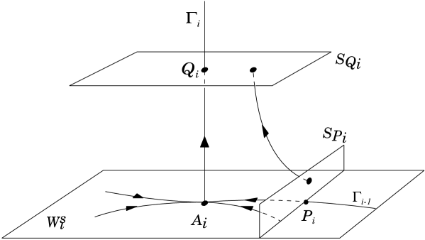
Figure 2: The local map in a neighborhood of a saddle point.

The proof of the theorem is based on the construction of the Poincaré map along orbits in a neighborhood of the contour $\Gamma$. Let $W_{i}^{s}$ ($W_{i}^{u}$) be a stable (unstable) manifold of the point $A_{i}$ and $P_{i}$ ($Q_{i}$) be a point on the heteroclinic orbit $\Gamma_{i-1}$ ($\Gamma_{i}$) in a small neighborhood of $A_{i}$–see Fig 2.

3.2.1 Local map

Let $S_{P_{i}}$ ($S_{Q_{i}}$) be a piece of a transversal to $\Gamma_{i-1}$ (to $\Gamma_{i}$) hyperplane going through $P_{i}$ (through $Q_{i}$). Without loss of generality, we may assume that $S_{P_{i}}$ is a piece of a hyperplane, parallel to the hyperplanes ${a_{i+1=0}}$. A local map $f_{i}:S_{P_{i}}\rightarrow S_{Q_{i}}$ along orbits in a neighborhood of $A_{i}$ is well defined. In suitable coordinates it has the form [Shilnikov et al., 2001].

$$\xi_{i}=c_{i}\eta_{i}^{\nu_{i}},\chi_{i}=\varphi_{i}(y_{i},\eta_{i})$$ (12)

where $\eta_{i}\in\Re$ is a coordinate on $S_{P_{i}}$, “parallel” to $W_{i}^{u}$, $y\in\Re^{N-2}$ is a vector-coordinate transversal to the $\eta_{i}$-axis on $S_{P_{i}}$, $\xi_{i}$ is a coordinate on $S_{Q_{i}}$, “parallel” to the leading direction on $W_{i}^{S}$ at $A_{i}$, $y_{i}$ is a vector-coordinate transversal to the $\xi_{i}$-axis on $S_{Q_{i}}$. Moreover,

$$|\frac{\partial\varphi_{i}}{\partial y_{i}}|\leq\bar{c}_{i}\eta_{i}^{\beta_{i}},|\frac{\partial\varphi_{i}}{\partial\eta_{i}}|\leq\bar{c}_{i}|y_{i}|\cdot|\eta_{i}|^{\beta_{i}-1}$$ (13)

where $\bar{c}_{i}>0$ is a constant and

$$\beta_{i}>\nu_{i}$$ (14)

3.2.2 Global map

The heteroclinic orbit $\Gamma_{i}$ has a piece joining the points $Q_{i}$ and $P_{i+1}$. Thus, the global map $F_{i}:\tilde{S}_{Q_{i}}\rightarrow S_{P_{i+1}}$ along orbits in a neighborhood of this piece is well-defined where $\tilde{S}_{Q_{i}}\subset S_{Q_{i}}$ is a small neighborhood of the point $Q_{i}$ on $S_{Q_{i}}$. This map is a diffeomorphism and has the form

$$\eta_{i+1} = a_{i1}\xi_{i}+a_{i2}\xi_{i}+...$$

$$y_{i+1} = b_{i0}+b_{i1}\xi_{i}+b_{i2}\xi_{i}+...\quad,$$ (15)

where the dots denote nonlinear terms. The orbit $\Gamma_{i}$ belongs to the intersection of invariant hyperplanes $\{a_{j}=0\}$, $j\neq i$, $j\neq i+1$. Therefore the hyperplane $\{\xi_{i}=0\}$ on $S_{Q_{i}}$ is mapped by $F_{i}$ into the hyperplane $\{\eta_{i+1}=0\}$ on $S_{P_{i+1}}$ which means that $a_{i2}=0$ in (15), and

$$a_{i1}\neq 0$$ (16)

Hence (15) has the form:

$$\eta_{i+1} = a_{i}\xi_{i}+...$$

$$y_{i+1} = b_{i0}+b_{i1}\xi_{i}+b_{i2}\xi_{i}+...\quad,$$ (17)

$a_{i1}=:a_{i}$.

3.2.3 Poincaré map

We may construct a Poincaré map $F=S_{P_{1}}\rightarrow S_{P_{1}}$ as the superposition of maps $f_{i}$, $F_{i}$, i.e. $F$ has the form $F=F_{N}\cdot f_{N}\cdot...\cdot F_{2}\cdot f_{2}\cdot F_{1}\cdot f_{1}$.

The map $F_{i}\circ f_{i}$ has the form

$$\eta_{i+1} = a_{i}c_{i}\eta_{i}^{\nu_{i}}+...$$

$$y_{i+1} = b_{i0}+b_{i1}c_{i}\eta_{i}^{\nu_{i}}+b_{i2}\varphi_{i}(y_{i},\eta_{i})+...$$ (18)

So, in this approximation the form of the map $F$ along the $\eta$-coordinates is independent of the $y$-coordinates , and one may consider the one-dimensional approximation

$$\eta_{i+1} = a_{i}c_{i}\eta_{i}^{\nu_{i}},i=1,...,N$$ (19)

$$\eta_{N+1} := \bar{\eta}_{1}\equiv\tilde{F}(\eta_{1})$$

It is simple to see that the map $\tilde{F}:\eta_{1}\rightarrow\bar{\eta}_{1}$ is a contraction provided that condition (11) is satisfied. Indeed, it follows from (19) that $\bar{\eta_{1}}=A\eta_{1}^{\nu}$, where $A$ is a constant and $\nu=\prod_{i=1}^{N}\nu_{i}$. Hence if $\nu>1$, then $\partial\bar{\eta_{1}}/\partial\eta_{1}<1$ if $\eta_{1}$ is small enough, the map (19) is a contraction and $\eta_{1}=0$ is an attracting fixed point (corresponding to the contour $\Gamma$).

Consider now the map $F_{i}\circ f_{i}$. The differential

$$DF_{i}\circ f_{i}=\left(\begin{array}[]{ll}a_{i}c_{i}\nu_{i}\eta_{i}^{\nu_{i}-1}+...&0+...\\ b_{i1}c_{i}\nu_{i}\eta_{i}^{\nu_{i}-1}+b_{i2}\frac{\partial\varphi_{i}}{\partial\eta_{i}}+...&\frac{\partial\varphi_{i}}{\partial y_{i}}+...\end{array}\right)$$ (22)

and because of (13), (14),

$$\|DF_{i}\circ f_{i}\|\leq B_{i}\eta_{i}^{\nu_{i}-1}$$ (23)

where $B_{i}$ is a constant. Since $DF=\prod_{i=1}^{N}D(F_{i}\circ f_{i})$, then

$$\|DF\|\leq B\prod_{i=1}^{N}\eta_{i}^{\nu_{i}-1}$$ (24)

where $B=\prod_{i=1}^{N}B_{i}$. We estimate now $\prod_{i=1}^{N}\eta_{i}^{\nu_{i}-1}$ by using (18). In the expression $\eta_{N}^{\nu_{N}-1}\cdot\eta_{N-1}^{\nu_{N-1}-1}\cdot...\cdot\eta_{2}^{\nu_{2}-1}\cdot\eta_{1}^{\nu_{1}-1}$ let us estimate first $\eta_{2}^{\nu_{2}-1}\cdot\eta_{1}^{\nu_{1}-1}$. Since $\eta_{2}=a_{1}c_{1}\eta_{1}^{\nu_{1}}+...$, then $\eta_{2}^{\nu_{2}-1}\cdot\eta_{1}^{\nu_{1}-1}=(a_{1}c_{1})^{\nu_{2}-1}\cdot(\eta_{1}^{\nu_{1}}+...)^{\nu_{2}-1}\cdot\eta_{1}^{\nu_{1}-1}\leq{\mbox{c}onst}\cdot\eta_{1}^{\nu_{1}\nu_{2}-1}$.

Now $\eta_{3}^{\nu_{3}-1}\cdot\eta_{2}^{\nu_{2}-1}\cdot\eta_{1}^{\nu_{1}-1}=(a_{2}c_{2})^{\nu_{3}-1}\cdot(\eta_{2}^{\nu_{2}}+...)^{\nu_{3}-1}\cdot\eta_{1}^{\nu_{1}-1}\leq const\cdot\eta_{2}^{\nu_{3}\nu_{2}-1}\cdot\eta_{1}^{\nu_{1}-1}={\mbox{c}onst}\cdot(a_{1}c_{1})^{\nu_{3}\nu_{2}-1}(\eta_{1}^{\nu_{1}}+...)^{\nu_{3}\nu_{2}-1}\cdot\eta_{1}^{\nu_{1}-1}\leq{\mbox{c}onst}\cdot\eta_{1}^{\nu_{3}\nu_{2}\nu_{1}-1}$.

Assume (inductively) that $\eta_{k}^{\nu_{k}-1}\cdot...\cdot\eta_{2}^{\nu_{2}-1}\leq{\mbox{c}onst}\cdot\eta_{2}^{\nu_{k}...\nu_{2}-1}$, then $\eta_{k}^{\nu_{k}-1}\cdot...\cdot\eta_{2}^{\nu_{2}-1}\cdot\eta_{1}^{\nu_{1}-1}\leq{\mbox{c}onst}\cdot(a_{1}c_{1}\eta_{1}^{\nu_{1}}+...)^{\nu_{k}...\nu_{2}-1}\cdot\eta_{1}^{\nu_{1}-1}\leq{\mbox{c}onst}\cdot\eta^{\prod_{i=1}^{k}\nu_{i}-1}$

and therefore,

$$\prod_{i=1}^{N}\eta_{i}^{\nu_{i}-1}\leq C\cdot\eta_{1}^{\nu-1}$$ (25)

where $C$ is a constant. Hence,

$$\|DF\|\leq BC\eta_{1}^{\nu-1},$$ (26)

i.e. $F$ is a contraction in a neighborhood of the point $\eta_{1}=0$, $y_{1}=0$ corresponding to the contour $\Gamma$.

This concludes the proof of Theorem 1.

3.3 Selecting the Contour

In this subsection we show how the canonical system (2) can be obtained from a general system for a neural network with inhibitory connections. Suppose that the dynamics of a network of $N+M$ inhibitory neurons with dynamical variables $y_{i}(t)=(y_{i}^{(1)}(t),...,y_{i}^{(m)}(t)),i=1,...,N+M$ can be described in the form of the following system of ODEs:

$$\dot{y}_{i} = F(y_{i})-\sum_{j=1}^{N+M}G_{ij}(s)(y_{i},y_{j})+\tilde{S}_{i}(t)$$ (27)

where $F$ is a nonlinear function that describes dynamics of individual neuron, $G_{ij}(S)(y_{i},y_{j})$ is a nonlinear operator describing an inhibitory action of the $j$-th neuron onto the $i$–th neuron, $S(t)=(S_{1}(t),...,S_{N+M}(t))$ and $(\tilde{S}_{1}(t),...,\tilde{S}_{N+M}(t))$ are the vectors representing stimuli to the network. We restrict ourselves to a subclass of systems (27) represented in the form (1). It is known (see above) that a stimulus acts in two ways: (i) it adds the perturbation $\tilde{S}(t)$ into (27) as an external force, and (ii) it forms the matrix $G_{ij}(S)$. A simplified model that describes the firing rate of the neurons can be written in the form (1) [Rabinovich et al., 2001], where $\sigma=-1$ when there is no stimulus, and $\sigma=1$ when the stimulus has a component at neuron $i$. In the absence of the external force $\tilde{S}(t)$ the system (2) is just a subsystem of (1) for which all $\sigma=+1$.

We describe now an algorithm to obtain the system (2) from (1) (provided that $\tilde{S}(t)=0$). First of all we single out only indexes $i$ for which $\sigma_{i}(S)=+1$. As a result we obtain a system which has the form:

$$\dot{a}_{i} = a_{i}[1-(a_{i}+\sum_{i\neq j}^{N+M_{1}}\rho_{ij}a_{j})]$$ (28)

with $M_{1}\leq M$. Then we consider the only those indexes $i$ for which conditions (3) and (4) are satisfied. After some permutation we have the system

$$\dot{a}_{i} = a_{i}[1-(a_{i}+\sum_{i\neq j}^{N+M_{2}}\rho_{ij}a_{j})]$$ (29)

with $M_{2}\leq M_{1}$. Let us form a graph $G$ now: its nodes are equilibrium points of (29), e.g. points $A_{i}=(0...0i=10...)$. There is an edge starting at the point $A_{i}$ and ending at the point $A_{j}$ if there is a separatrix (a piece of $W_{i}$) joining and $A_{i}$ and $A_{j}$. Thus, for any point $A_{i}$ there is the only one edge starting at $A_{j}$. It implies that there exists a subgraph of this graph in the form of a cycle that contains, say, $N$ vertices. The equation describing dynamics of $N$ corresponding neurons has exactly the form (2) (maybe after some permutative change of variables).

4 Birth of a Stable Limit Cycle

A direct corollary of Theorem 1 is the possibility of the birth of the stable limit cycle in system (2) when perturbed in an appropriate way. A perturbation should act in such a way that a Poincaré map $S_{P_{1}}\rightarrow S_{P_{1}}$ for the perturbed system has an absorbing region and a fixed point inside it. Such a condition can be expressed differently. Let us do it as follows. Consider the system

$$\dot{a}_{i}=a_{i}[1-(a_{i}+\sum_{j\neq i}^{N}\rho_{ij}a_{j})]+\epsilon\Psi_{i}(a)$$ (30)

that coincides with (2) for $\epsilon=0$, where $a=(a_{1},...,a_{N})$ and $\Psi_{i}$ is a smooth function, $i=1,...,N$. For small $\epsilon>0$ the system (30) has saddle equilibrium points $A_{i\epsilon}$ and separatrices $\Gamma_{i\epsilon}$ (the half of $W_{i\epsilon}^{u}$ such that $A_{i\epsilon}\rightarrow A_{i}$, as $\epsilon\rightarrow 0$ and $lt_{\epsilon\rightarrow 0}\Gamma_{i\epsilon}\supset\Gamma_{ii+1}$ (here $lt$ means the topological limit, i.e. the set of the accumulation points).

Theorem 2

Assume that the conditions of Theorem 1 are satisfied,

$$lt_{\epsilon\rightarrow 0}(\bigcup_{i=1}^{N}\Gamma_{i\epsilon})=\Gamma$$ (31)

and at least one of the separatrices $\Gamma_{i\epsilon}$ is not a heteroclinic orbit. Then for any sufficiently small $\epsilon>0$ the system (30) has a stable limit cycle $L_{\epsilon}$ (in a neighborhood of $\Gamma$) such that $lt_{\epsilon\rightarrow 0}L_{\epsilon}=\Gamma$.

The proof of this Theorem can be done in the standard way, i.e., by construction of the Poincaré map and by showing (as in the proof of Theorem 1) that this map is a contraction in an absorbing region. The condition (31) (or a similar condition) is necessary and sufficient for the existence of an absorbing region. We omit the proof in the present work, since it is really a standard one (the corresponding technique can be found in [Shilnikov et al., 2001, Afraimovich et al., 1998, Afraimovich et al., 2001]. Thus, one may say that the system under consideration is robust in the following sense: the attractor of a perturbed system remains in a small neighborhood of the “unperturbed” attractor.

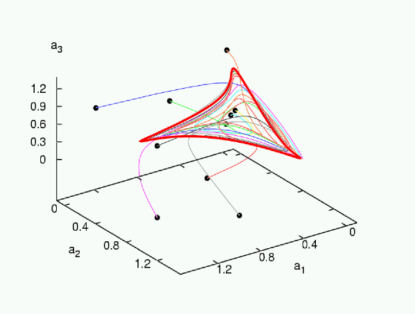
Figure 3: 3D projection of the 6-dimensional system (32) showing examples of trayectories falling into the limit cycle from different initial conditions. As the numerical results indicate, this limit cycle in the vicinity of the former heteroclinic contour is a global attractor

Numerical results show that the system (30) where $\Psi_{i}(a)\geq 0$ satisfies the condition (31) and has a stable limit cycle. An example is shown in Fig. 3. In particular, it is clear from this figure that the system has the only one -global- attractor. In this example, the simulations were performed with the following equations:

$$\dot{a_{i}} = a_{i}(1-\sum_{j=1}^{N=6}\rho_{ij}a_{j})+\epsilon a_{i}a_{i+3}$$ (32)

where $i=1,2,...,6$ and $i+3\equiv i-3$ if $i>3$. We used the following values of the connection matrix $\rho_{ij}\neq 0$:

$$\rho_{1,3} = \rho_{3,5}=\rho_{5,1}=5;\hskip 5.69054pt\rho_{4,6}=\rho_{2,4}=\rho_{6,2}=2$$

$$\rho_{1,6} = \rho_{2,1}=\rho_{3,2}=\rho_{4,3}=\rho_{5,4}=\rho_{6,5}=1.5$$

$$\rho_{1,1} = \rho_{2,2}=\rho_{3,3}=\rho_{4,4}=\rho_{5,5}=\rho_{6,6}=1$$ (33)

with $\epsilon=0.01$.

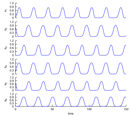
Figure 4: Time series showing the switching of activities $a_{i}$ in a network of six neurons described by equations (32). Units are dimensionless. See parameters used in the text.

Time series showing the switching of activities displayed in this system by the WLC are depicted in Fig. 4.

5 WLC in Real Neural Systems

In this section we describe two examples of living neural systems that appear to use WLC strategies to process sensory information. As we discussed in the Introduction, sensory systems need both robustness and sensitivity to acquire and process incoming signals. The WLC among sensory neurons guarantees the coexistence of these essential characteristics and can explain the experimental recordings in several sensory systems. We will illustrate two of these sensory systems using models with WLC dynamics.

5.1 WLC in Olfactory Processing

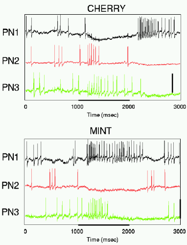
Figure 5: Temporal patterns produced by three simultaneously sampled PNs in the locust antennal lobe when two different odors are presented during the time interval from 1000 to 2000 msec. The horizontal bar indicates the time interval when the stimulus was presented (see [Wehr & Laurent, 1996] for details).

Observed features of olfactory processing networks [Wehr & Laurent, 1996, Laurent et al., 2001] can guide the study of computation using competitive networks. In Fig. 5 we show the simultaneously recorded activity of three different projection neurons (PNs) in the locust olfactory system, i.e. antennal lobe (AL), evoked by two different odors: despite similar PN activities before the stimulus onset (the result of the action of noise) each odor evokes a specific spatio-temporal activity pattern that results from interactions between these and other neurons in the network [Laurent et al., 2001, Bazhenov et al., 2001, Rabinovich et al., 2000b].

As we have discussed, WLC networks produce identity-temporal or spatio-temporal coding in the form of deterministic trajectories moving along heteroclinic orbits that connect saddle fixed points or saddle limit cycles (see Fig. 1) in the system’s state space. These saddle states correspond to the activity of specific neurons or groups of neurons and the separatrices connecting these states correspond to sequential switching from one state to another.

From the experimental results [Wehr & Laurent, 1996, Laurent et al., 2001] we infer that a stimulus acts in two principal ways: (1) it excites a subset of projector neurons; (2) it modifies the effective inhibitory connections between the projector neurons as a result of activation of the inhibitory interneurons that connect different PNs. The intrinsic dynamics of these neurons is governed by many variables corresponding to ion channels and intracellular processes. Such detailed description however is not needed to illustrate the principle of “coding with separatrices”. We need only to capture the ‘firing’ or ‘not-firing’ state of the component neurons. We thus simplify our model to an equation for the firing rate $a_{i}(t)>0$ of neural activity [Rabinovich et al., 2000b]:

$$\dot{a}_{i}(t)=a_{i}(t)\bigg{[}\sigma_{i}({\bf S})-\bigg{(}a_{i}+\sum_{j\neq i}^{N}\rho_{ij}({\bf S})a_{j}(t)\bigg{)}\bigg{]}+S_{i}(t).$$ (34)

where $\rho_{ij}({\bf S})$ is the strength of inhibition of neuron $j$ onto $i$. $\sigma_{i}({\bf S})=-1$, when there is no stimulus, and $\sigma({\bf S})=+1$ when the stimulus has a component at neuron $i$. When $\sigma_{i}=-1$, the quiet resting state $a_{i}=0$ is stable. When a stimulus is applied and $\sigma_{i}=+1$, the system moves away from this quiet state onto a sequence of heteroclinic trajectories. This instability triggers the system into rapid action, provides robustness against noise and allows a response independent of the state at stimulus onset.

When the inhibitory connections are not symmetric, the system with $N$ competitive neurons has different closed heteroclinic orbits that consist of saddle points and one dimensional separatrices connecting them. Such heteroclinic orbits are global attractors in phase space and are found in various regimes of the $\rho_{ij}({\bf S})$. This implies that if the stimulus is changed, another orbit in the vicinity of the heteroclinic orbit becomes a global attractor for this stimulus. Such rich behavior can be illustrated also by an inhibitory ensemble of spiking neurons. We have studied a network of inhibitory connected FitzHugh-Nagumo neurons ($i=1,2,...,9$) [Rabinovich et al., 2000b]:

$$\tau_{1}\frac{dx_{i}(t)}{dt} = f(x_{i}(t))-y_{i}(t)-z_{i}(t)(x_{i}(t)-\nu)+0.35+S_{i}$$

$$\frac{dy_{i}(t)}{dt} = x_{i}(t)-by_{i}(t)+a$$

$$\tau_{2}\frac{dz_{i}(t)}{dt} = \sum_{j}g_{ji}G(x_{j}(t))-z_{i}(t)$$ (35)

Here we use a dynamical model of inhibition: $z_{i}(t)$ is a synaptic current modeled by first order kinetics. The variable $x_{i}(t)$ denotes the membrane potential, $y_{i}(t)$ is a recovery variable, and $f(x)=x-\frac{1}{3}x^{3}$ is the internal FN nonlinearity. The stimulus is taken as a constant. We use a step function for $G(x)=0,x\leq 0,\mbox{and}\,G(x)=1,x>0$, as the synaptic connection. $S_{i}$ is the stimulus, and $g_{ji}$, the strength of synaptic inhibition: $g_{ji}=2$ if the $j^{th}$ neuron inhibits the $i^{th}$; $0$ otherwise. The other parameters are $a=0.7,b=0.8,\tau_{1}=0.08,\tau_{2}=3.1,\nu=-1.5$.

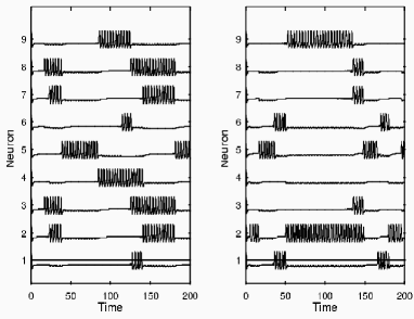
Figure 6: Spatio-temporal patterns generated by a network of nine FitzHugh-Nagumo neurons with inhibitory connections. We used the external stimuli: $S_{1}=0.1$, $S_{2}=0.15$, $S_{3}=0$, $S_{4}=0$, $S_{5}=0.15$, $S_{6}=0.1$, $S_{7}=0$, $S_{8}=0$, $S_{9}=0$, $\tau_{2}=3.1$ (left), and $S_{1}=0.01$, $S_{2}=0.03$, $S_{3}=0.05$, $S_{4}=0.04$, $S_{5}=0.06$, $S_{6}=0.02$, $S_{7}=0.03$, $S_{8}=0.05$, $S_{9}=0.04$, $\tau_{2}=4.1$ (right). We plot $x_{i}(t)$ versus time.

Our numerical simulations show that the network produces different spatio-temporal patterns in response to different stimuli. Fig. 6 presents examples of these activities corresponding to two different stimuli. The system was in the resting state $x_{i}\approx-1.2,y_{i}\approx-0.62,z_{i}=0$ before the stimulus began at $t=0$. As one can see, the patterns are considerably different and distinguishable. The heteroclinic contour in this network consists of a finite number of saddle limit cycles and the same number of heteroclinic orbits connecting these cycles (see, as an example, Fig. 1, right panel). A detailed characterization of this network as an information processing device has been reported in [Rabinovich et al., 2001].

5.2 WLC in the Gravimetric Neurons of the Mollusk Clione

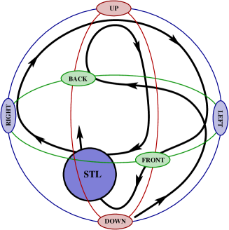
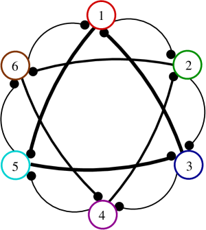
Figure 7: Left panel: Schematic representation of the statolith motion inside the statocyst, the gravimetric organ of the mollusk Clione. Right panel: inhibitory connections used in the network model of the statocyst receptor neurons (thicker traces mean stronger inhibition).

Neural networks with WLC dynamics are able to generate new information to answer a simple external signal. Such information can be used for the organization of complex activity and, in particular, chaotic behavior of some animals. Let us consider now the hunting activity of a marine mollusk Clione. This mollusk is a predator lacking a visual system. It feeds on a small mollusk, Limacina. The hunting behavior is a random search for prey: Clione ”scans” the surrounding space in order to locate and catch the prey. Such behavior is turned on by the smell of the Limacina. The main role in the organization of such motion of Clione is played by a sensory neural network inside the gravimetric organs: the statocysts (see Fig.7). These special sensory organs are responsible for the orientation in the gravitational field [Arshavsky et al., 1993].

It is well known from the physiological data that the statocysts have up to 12 receptor neurons (SRNs) that are coupled with inhibitory synapses [Arshavsky et al., 1993]. These neurons respond to the pressure exerted by the statolith, a stone located inside the statocyst. If no information about a prey (received by the chemical receptors) is present, the receptor neuron $D$ (down, see Fig. 7) is excited by the statolith and it inhibits other SRNs, and the network responds in a winner-take-all mode. As a result, the information generated by $D$ SRN arrives to the corresponding Central Pattern Generators (CPGs) that control the tail and wing movements. These CPGs establish the habitual ”head up” position of Clione’s body. However if a special Hunting Central Neuron (HCN) receives a message from the chemo-sensors about the presence of a prey, HCN excites the SRNs organizing a WLC among them as we will illustrate with a model. The behavior of the Clione in this case does not depend on the direction of the gravitational field and it moves in a random-like trajectory.

For the phenomenological modeling of the statocyst “hunting” dynamics we can neglect the statolith inertial dynamics and take into account the only key point: the position of the mollusk’s body uniquely depends on the message that SRNs are sending to the central neurons that produce the commands to the CPGs. Thus, as a starting point, we consider just a SRN network under the action of the HCN excitation. We suppose that, as a result of the HCN stimulation, all SRNs (”left”, ”right”, ”back”, ”front”, ”down”, and ”up”) are in the same situation: they receive and send two inhibitory synapses (see Fig. 7, right panel).

The dynamics of the SRN’s network can be described by model (1) with $N=6$. In this case, $a_{i}>0$ represents the instantaneous spiking rate of the receptor neuron $i$, $H_{i}(t)$ represents the stimulus from the hunting neuron to neuron $i$, and $S_{i}(t)$ represents the action of the statolith on the receptor that is pressing. When there is no stimulus from the hunting neuron ($H_{i}=0,\forall i$) or the statolith ($S_{i}=0,\forall i$), then $\sigma(\mbox{\boldmath$H$},\mbox{\boldmath$S$})=-1$ and all neurons are silent; $\sigma(\mbox{\boldmath$H$},\mbox{\boldmath$S$})=1$ when the hunting neuron is active and/or the statolith is pressing one of the receptors. In our simulations, we have used the values $\rho_{ij}\neq 0$ specified in (33).

When there is no activation of the sensory neurons from the hunting neuron, the effect of the statolith ($S_{i}\neq 0$) in this model is to induce a higher rate of activity on one of the neurons (the neuron $i$ where it rests for a big enough $S_{i}$ value). We assume that this higher rate of activity affects the behavior of the motoneurons to organize the head up position. The other neurons are either silent or have a lower rate of activity and we can suppose that they do not influence the posture of Clione.

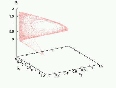
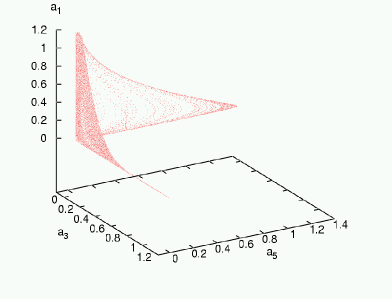
Figure 8: Projections of the attractor from the six-dimenional phase space of the statocyst receptor network to two different three-dimensional spaces.

When the hunting neuron is active a completely different behavior arises. We assume that the action of the hunting neuron overrides the effect of the statolith and thus $S_{i}\approx 0,\forall i$. The dynamical system (1) with the $\rho_{ij}$ values specified above (see also Fig. 7) and with a stimuli from the hunting neuron given, for example, by $H_{i}=(0.730,0.123,0.301,0.203,0.458,0.903)$ has a strange attractor in the phase space (see Fig. 8). This means that the SRN network generates new information (a chaotic signal with positive Kolmogorov-Sinai entropy) in the presence of the prey, which controls the CPGs and, in fact, organizes the random-like behavior of Clione.

The origin of the chaoticity in such dynamical system can be explained in the following manner [Varona et al., 2001]: due to the diversity in the strengths of the inhibitory connections we may consider the complete network as two weakly coupled WLC triangle networks. Independently each of them has a closed heteroclinic contour (see Fig. 7), which becomes a limit cycle under the action of a small perturbation (see Sec. 4). The periodic oscillations corresponding to these limit cycles have, in general, different frequencies that are extremely sensitive to the distance to the heteroclinic loop in the non perturbed system (such oscillations are strongly non-synchronous). As we showed the weak interaction of these WLC triangles (nonlinear oscillators) generate chaos in wide regions of the control parameter space. New experiments have confirmed the validity of the model and its predictions [Levi et al., 2002].

6 Discussion

The stimulus dependent sequential switching of neurons or group of neurons (clusters), named WinnerLess Competition, is able to solve the fundamental contradiction between sensitivity and robustness of the sensory recognition. The key points on which the WLC networks are based are: (i) the heteroclinic contour corresponding to a specific sequence of switching has a large basin of attraction, i.e. a specific sequence is stable; and (ii) the topology of the heteroclinic contour sensitively depends on the incoming signals, i.e. high resolution or sensitivity. Both features are actually present only in the case if under the action of a perturbation the discussed heteroclinic contour, which is structurally unstable, is transformed to the limit cycle in its vicinity with the same topology as the contour. In this paper we have discussed the conditions for such topological stability, and we have showed that computing with separatrices based on the WLC principle is a very natural and powerful strategy for information processing in real neural systems. Any kind of sequential activity can be programmed by a network with stimulus dependent nonsymmetric inhibitory connections. It can be the creation of spatio-temporal patterns of motor activity, the transformation of the spatial information into spatio temporal information for successful recognition and many other computations. In addition, we wish to mention that two important computational functions can be successfully implemented by computation with separatrices. These are: (i) sequential memory storage, and (ii) feature binding.

In reference [Seliger et al., 2003] the authors suggest a new biologically-motivated model of sequential spatial memory which is based on the WLC principle. Each stimulus event (visual image, odor, etc…) is represented by a saddle point in the phase space of the system, and a network of one-dimensional separatrices leads the system along the sequence of events in the specific episode. After the learning process, such system is capable of an associative retrieval of the pre-recorded sequence of spatial patterns.

A binding problem occurs when two (or more) different events, e.g. scenes, features, or behaviors are represented by different neural ensembles simultaneously, and for some reason they are all connected with each other. Eventually, these coherent features are integrated by the nervous system of the animal onto a perceptual object, even if the features are dispersed among different sensory systems or subsystems. The binding is ubiquitous and occurs whenever a simultaneous remembrance or representation is important. The most common approach in the modeling of binding is to involve time in operation (von der Malsburg, Singer, and others). The idea is to use the coincidence of certain events in the dynamics of different neural units for binding. This is a dynamic binding. Usually, dynamic binding is represented by synchronous neurons or neurons that are in resonance with and external field. However, dynamical events like phase or frequency variations usually are not very reproducible and robust. It is reasonable to hypothesize that brain circuits that display sequential switching of neural activity [Abeles et al., 1995] use the coincidence of this switching to implement dynamic binding of different WLC networks.

In the conclusion we have to emphasize that for large inhibitory neural ensembles it is not necessary to have specific connections that satisfy the conditions formulated above for the existence and stability of the WLC dynamics. If the connections are random, the neurons in the ensemble can be separated in three groups: (i) neurons that are weakly coupled with others (they behave like nearly independent elements), (ii) neurons with strong but close to symmetric connections (they form a Hopfield like network just with simple attractors), and (iii) neurons with nonsymmetric connections that demonstrate the WLC dynamics. Because the WLC dynamics is a structurally stable phenomenon, it is reasonable to hypothesize that the perturbation of the third group by the first two does not destroy the switching activity. Recent computer experiments [Zhigulin, 2002] have confirmed this hypothesis.

ACKNOWLEDGMENTS

Support for this work came from NIH grant 2R01 NS38022-05A1, Department of Energy grant DE-FG03-96ER14592 and NSF/EIA-0130708. V.A. was supported by CONACyT grant 485100-3-36445-E and by UC MEXUS-CONACyT grant. P.V. was supported by MCyT BFI2000-0157.

References

- [Abeles et al., 1995] Abeles M., Bergman H., Gat I., Meilijson I., Seidemann E., Tishby N., Vaadia E., “Cortical Activity Flips Among Quasi-Stationary States,” Proceedings of The National Academy of Sciences of The United States Of America, 92 (N19): 8616-8620 (1995).
- [Afraimovich et al., 1998] Afraimovich V.S., Hsu S.-B., 1998, Lectures on Chaotic Dynamical Systems, National Tsing-Hua University, Hsinchu, Taiwan.
- [Afraimovich et al., 2001] Afraimovich V.S., Hsu S.B., Lin H.E., “Chaotic behavior of three competing species of May-Leonard model under small periodic perturbations”, International Journal of Bifurcation and Chaos 11(2), 435–447 (2001).
- [Arshavsky et al., 1993] Arshavsky Y.I., Orlovsky G.N., Panchin Y.V., Roberts A., Soffe S.R., “Neuronal control of swimming locomotion: analysis of the pteropod mollusc Clione and embryos of the amphibian Xenopus”, Trends Neurosci. 16: 227-233 (1993).
- [Arshavsky, 2002] Arshavsky Y., private communication.
- [Ashwin and Chossat, 1998] Ashwin P. and Chossat P., “Attractors for robust heteroclinic cycles with continua of connections”, J. Nonlinear Sci., 8, 103 (1998).
- [Ashwin and Field, 1999] Ashwin P. and Field M., “Heteroclinic network in coupled cell systems”, Arch. Rational Mech. Anal. 148, 107 (1999).
- [Bazhenov et al., 2001] Bazhenov M., Stopfer M., Rabinovich M.I., Abarbanel H.D.I., Sejnovski T.J. and Laurent G., “Model of cellular and network mechanisms for odor-evoked temporal patterning in the locust antennal lobe”, Neuron, 30(1) (2001).
- [Busse & Heikes, 1980] Busse, F.H. and Heikes, K.E. “Convection in a rotating layer: A simple case of turbulence”, Science 208, 173 (1980).
- [Chi et al., 1998] Chi C.W., Hsu S.B., Wu L.I., “On the asymmetric May-Leonard model of three competing species”, SIAM J. Appl. Math. 58(1), 211–226 (1998).
- [Cohen & Grossberg, 1983] Cohen M.A., Grossberg S., “Absolute stability of global pattern formation and parallel memory storage by competitive neural networks”, IEEE Transactions on Systems, Man and Cybernetics, vol. SMC-13, 5, 815–26 (1983).
- [Hopfield, 1982] Hopfield J.J., “Neural networks and systems with emergent selective computational abilities”, Proc. Natl. Acad Sci. USA 79, 2554–8 (1982).
- [Küppers & Lortz, 1969] Küppers G. and Lortz D. “Transition ofrom laminar convection to thermal turbulence in a rotating fluid layer”, J. Fluid Mech. 35, 609 (1969).
- [Laurent et al., 2001] Laurent G., Stopfer M., Freidrich R.W., Rabinovich M.I., Volkovskii A., and Abarbanel H.D.I., “Odor encoding as an active, dynamical process: experiments, computation and theory”, Ann. Rev. Neurosc. 24, 263 (2001).
- [Levi et al., 2002] Levi R., Varona P., Rabinovich M.I., Selverston A.I., Arshavsky Y.I., “Control of hunting behavior in the mollusk Clione: winnerless competition between the statocyst receptor neurons”, SFN Abstracts 28 60.1 (2002).
- [May & Leonard, 1975] May, R.M. and Leonard, W. J.“Nonlinear aspects of competition between three species”, SIAM, J. Appl. Math 29, 243 (1975).
- [Orlovsky et al., 1999] G.N. Orlovsky, T.G. Deliagina, S. Grillner, Neuronal Control of Locomotion. From Mollusc to Man, Oxford University Press (1999).
- [Rabinovich et al., 2000a] Rabinovich M.I., Ezersky A.B., and Weidman P.D. The Dynamics of Patterns, World Scientific, 2000a, 324p.
- [Rabinovich et al., 2000b] Rabinovich M.I., Huerta R., Volkovskii A., Abarbanel H.D.I., Stopfer M., Laurent G., “Dynamical coding of sensory information with competitive networks”, J. Physiol. (Paris) 94 465 (2000b).
- [Rabinovich et al., 2001] Rabinovich M.I., Volkovskii A., Lecanda P., Huerta R., Abarbanel H.D.I., Laurent G., “Dynamical encoding by networks of competing neuron groups: Winnerless competition”, Physical Review Letters 87(6), 068102–4 (2001).
- [Roy, 1999] Roy, R. private communication (1999).
- [Seliger et al., 2003] Seliger F., Tsimring L., Rabinovich, M.I., “Dynamical model of sequential spatial memory: winnerless competition of patterns”. In press for Phys. Rev. E.
- [Shilnikov et al., 2001] Shilnikov P., Shilnikov A.L., Turaev D.V., and Chua L.O., Methods of Qualitative Theory in Nonlinear Dynamics. Part II. World Scientific, Singapore, 2001.
- [Varona et al., 2001] Varona P., Rabinovich M.I., Selverston A.I., Arshavsky Y.I., “Winnerless competition between sensory neurons generates chaos: a possible mechanism for molluscan hunting behavior”. Chaos 12(3), 672–677 (2002).
- [Waltman, 1983] Waltman P., 1983, Competition Models in Population Biology, SIAM, PA, 1983.
- [Wehr & Laurent, 1996] Wehr, M. and Laurent, G. “Odour encoding by temporal sequences of firing in oscillating neural assemblies”, Nature 384, 162 (1996).
- [Zhigulin, 2002] Zhigulin, V. private commmunication (2002).