Functional sensitivity of Burgers and related equations to initial conditions

Abstract

In this paper, we apply sensitivity methods to nonlinear PDEs like Burgers and KPZ equations. These equations are known to have analytical solutions which make easier the analysis of the sensitivity of their solutions to initial conditions. The main result stands in the fact that the most the solution is sensitive to the initial condition, the most it is decorrelated in space, i.e. the values of the initial condition participate to the solution at all distances of the wave front. This finally reveals a particular aspect of the Burgers turbulence.

I Introduction

Burgers and related equations have been introduced in many fields of sciences such as non-equilibrium statistical physics. For instance, we can cite, in cosmology, the model known as the adhesion model cosmo , there is also the modeling of traffic jam jam , the description of directed polymers in random media newman ; medina or the dynamics of growing interface kpza . Note also that the Burgers equation may be a draft modeling to fluid dynamics.

When modeling a system by means of the Burgers or the KPZ equation knowledge of the initial condition is required. However a great insight of the problem is necessary in order to fit experimental data as soon as high quality results are available. It is then interesting to know the interdependence of the solution of the modeling equation to initial conditions. This is the goal of sensitivity analysis to provide the system response to variations of input volt ; fran . This mathematical method has been applied in numerous domains of sciences, see for instance rab ; hang .

For an initial value problem, such as the following evolution equation:

$$\partial_{t}u(x,t)=A\,u(x,t)\quad$$

$$u(x,0)=\varphi(x),\;x\in\mathbb{R},$$ (1)

where $A$ is some nonlinear operator, the variation $\delta\varphi(x)$ of the initial condition should imply variations $\delta u(x,t)$ in the solution $u(x,t)$ of the equation. These variations obey the functional relation:

$$\delta u(x,t)=\int_{-\infty}^{+\infty}\frac{\delta{u(x,t)}}{\delta{\varphi(y)}}\,\delta\varphi(y)\,{\rm{d}}y.$$ (2)

Then the functional derivative $\delta{u(x,t)}/\delta{\varphi(y)}$ (sometimes called the density) gives a quantitative measure of the response of the actual solution $u(x,t)$ to any variation of the input.

As said extensively in the literature, nonlinear and chaotic systems are mainly characterized by sensitivity to initial conditions. The purpose of the present paper is to quantify this sensitivity in the cases of Burgers and related equations.

II The heat equation

Before we treat the case of nonlinear equation, we shall examine in this section the case of the heat equation:

$$\partial_{t}Z=\nu\partial_{xx}Z,$$ (3)

with the initial condition: $Z(x,0)=\psi(x)$, and where $\nu$ is some diffusion parameter. We have the well known solution to the heat equation as the convolution integral:

$$Z(x,t)=\frac{1}{\sqrt{4\pi\nu t}}\int_{-\infty}^{+\infty}\psi(y)\,\exp\left[-\frac{(x-y)^{2}}{4\nu t}\right]\,{\rm{d}}y.$$ (4)

Now we can calculate the sensitivity coefficient, i.e. the functional derivative of the solution $Z(x,t)$ with respect to the initial condition $\psi(x)$ directly from this solution. It reads:

$$\frac{\delta{Z(x,t)}}{\delta{\psi(x^{\prime})}}=\frac{1}{\sqrt{4\pi\nu t}}\int_{-\infty}^{+\infty}\frac{\delta{\psi(y)}}{\delta{\psi(x^{\prime})}}\,\exp\left[-\frac{(x-y)^{2}}{4\nu t}\right]\,{\rm{d}}y.$$ (5)

As we have: $\frac{\delta{\psi(y)}}{\delta{\psi(x^{\prime})}}=\delta(x^{\prime}-y)$, the sensitivity coefficient is then given by:

$$\frac{\delta{Z(x,t)}}{\delta{\psi(x^{\prime})}}=\frac{1}{\sqrt{4\pi\nu t}}\exp\left[-\frac{(x-x^{\prime})^{2}}{4\nu t}\right].$$ (6)

We first remark that the density is well correlated along the line $x=x^{\prime}$ in the $(x,x^{\prime})$ plane and it does not involve the initial condition $\psi(x)$ itself. In fact, since the heat equation is linear, this density is also a solution to the heat equation with the initial condition $\delta(x-x^{\prime})$ (i.e. the fundamental solution). Moreover, as $t$ goes to infinity the sensitivity coefficient spreads and goes to zero. Consequently, the solution to the heat equation is asymptotically insensitive to initial conditions. This proves, as well, the known issue concerning the very high difficulty to find the initial condition from the measurement of $Z(x,t)$ at any time.

III The unforced Burgers equation

Let us recall, the chain of transformations leading to the solution of the unforced Burgers equation. The Burgers equation is given by:

$$\partial_{t}u+u\partial_{x}u=\nu\partial_{xx}u,$$ (7)

with the initial condition $u(x,0)=\varphi(x)$. Where $\nu$ stands usually for the viscosity coefficient. The change of function defined by $u(x,t)=-\partial_{x}h(x,t)$ leads to the KPZ equation kpza :

$$\partial_{t}h=\frac{1}{2}\left(\partial_{x}h\right)^{2}+\nu\partial_{xx}h,$$ (8)

with the corresponding initial condition $h(x,0)=\eta(x)$. Then the Hopf-Cole transformation: $h=2\nu\ln Z$, yields to the heat equation (Eq. (3)) kpza ; Hopf ; cole .

From the general solution of the heat equation (Eq. (4)), we find the solution to Eq.(8) as:

$$h(x,t)=2\nu\ln\left\{\frac{1}{\sqrt{4\pi\nu t}}\qquad\qquad\qquad\qquad\qquad\qquad\right.$$

$$\left.\quad\qquad\times\int_{-\infty}^{+\infty}\exp\left[\frac{1}{2\nu}\left(\eta(y)-\frac{(x-y)^{2}}{2t}\right)\right]\,{\rm{d}}y\right\}.$$ (9)

Taking the functional derivative of this equation, we obtain the sensitivity coefficient of $h(x,t)$ to the initial condition:

$$\frac{\delta{h(x,t)}}{\delta{\eta(x^{\prime})}}=\frac{\exp\left[\frac{1}{2\nu}\left(\eta(x^{\prime})-\frac{(x-x^{\prime})^{2}}{2t}\right)\right]}{\int_{-\infty}^{+\infty}\exp\left[\frac{1}{2\nu}\left(\eta(y)-\frac{(x-y)^{2}}{2t}\right)\right]\,{\rm{d}}y}.$$ (10)

On the contrary to the heat equation, the unforced KPZ equation solution is very sensitive to the initial condition, moreover this is also the case in the long time limit:

$$\lim_{t\to\infty}\frac{\delta{h(x,t)}}{\delta{\eta(x^{\prime})}}=\frac{\exp\left[\frac{1}{2\nu}\eta(x^{\prime})\right]}{\int_{-\infty}^{+\infty}\exp\left[\frac{1}{2\nu}\eta(y)\right]\,{\rm{d}}y},$$ (11)

where we assume the convergence of the integral. Surprisingly it does not depend on $x$. This means that, in the long time limit, the initial condition $\eta(x^{\prime})$ at the distance $x^{\prime}$ influences $h(x,t)$ for all the values of $x$ with the same weight. It is interesting also to look at the inviscid limit of this result. Assuming there is only one stationary point $a$, the sensitivity coefficient may written as:

$$\frac{\delta{h(x,t)}}{\delta{\eta(x^{\prime})}}{\xrightarrow{t\to\infty,\,\nu\to 0}}\sqrt{\frac{|h^{\prime\prime}(a)|}{4\pi\nu}}\exp\left[\frac{1}{2\nu}(\eta(x^{\prime})-\eta(a))\right].$$ (12)

Note these two limits do not act always uniformly. As $a$ corresponds to the maximum of $\eta(x)$, we see that the sensitivity coefficient is peaked on this value.

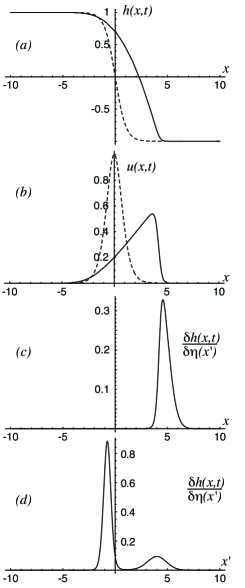
Figure 1: Plots of the solution to Eq. (9): (a) and of the solution to the Burgers equation (b) for the time $t=8$ in arbitrary units. The doted lines correspond to initial conditions. The sensitivity coefficients are plotted as function of $x$ on (c) and as function of $x^{\prime}$ on (d).

A simple example of illustration of these results may be given with the choice of the initial condition for the velocity in the Burgers equation as $u(x,0)={\rm{sech}}^{2}\,x$, so that the initial condition for $h$ is $h(x,0)=-\tanh\,x$. On Fig. (1 – a and b), we present the values of $h(x,t)$ and of the solution to the Burgers equation $u(x,t)$ for the time $t=8$ (given in arbitrary units) as functions of $x$. The dotted lines correspond to initial values of these functions. The viscosity is fixed to the rather small value: $\nu=0.05$. The sensitivity coefficient $\delta{h(x,t)}/\delta{\eta(x^{\prime})}$ as a function of $x$ is given on Fig. (1 – c) for a fixed value of $x^{\prime}=4$. We observe a maximum value of the sensitivity at the bottom of the wave front. This is also the case for the sensitivity coefficient as a function of $x^{\prime}$ where $x$ is also fixed to 4. However in this case, a higher maximum is found near the edge of the wave front on Fig. (1 – d). This suggests that the whole wave front is involved in the evolution. In fact, a better representation of the phenomena is found in the $(x,x^{\prime})$ plane of the sensitivity coefficient.

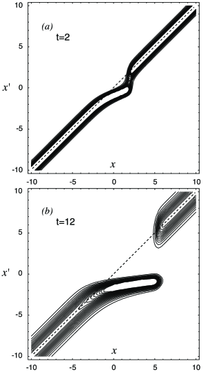
Figure 2: Contour plot of the sensitivity coefficient $\delta{h(x,t)}/\delta{\eta(x^{\prime})}$ in the $(x,x^{\prime})$ plane, for two values of time ($t=2$ and $t=12$). For a smaller value of time (a), the solution is rather well correlated to the initial condition except in a small region near the wave front. When the time increases (b), the density spreads and one can observe a decorrelation through along the wave front.

On Fig. (2), we present the contour plot of the sensitivity coefficient. The doted lines given on Fig. (2) correspond to the initial value of the density where the solution is perfectly correlated to the initial condition for $\delta{h(x,0)}/\delta{\eta(x^{\prime})}=\delta(x-x^{\prime})$. For a given value of $x^{\prime}$ and coming from large values of $x$ at time $t=2$ (Fig. (2–a)), the sensitivity is still well correlated until one reaches a breaking off near the bottom of the wave front showing perturbations appear. After an interval, larger as the time elapses ($t=12$, Fig. (2–b)), we observe a decorrelation through along the wave front. In the mean time, the sensitivity coefficient takes its larger values on this region. Behind the wave front, the density will be correlated again, although we constat a spreading when the time increases. For very large value of the time, the density is completely decorrelated as we said above with Eq. (11). In order to sum up these results, one can say that the most the solution is sensitive to the initial condition, the most it is decorrelated in space, i.e. all the values of the initial condition participate to the solution at any distance along the wave front. This finally reveals a characteristic of the Burgers turbulence.

Now we can find the sensitivity of the solution to the unforced Burgers equation by the same method. In order to do the calculation, we have on one hand:

$$\frac{\delta{u(x,t)}}{\delta{\varphi(x^{\prime})}}=\int_{-\infty}^{+\infty}\frac{\delta{u(x,t)}}{\delta{\eta(y)}}\frac{\delta{\eta(y)}}{\delta{\varphi(x^{\prime})}}\,{\rm{d}}y=\int_{x^{\prime}}^{+\infty}\frac{\delta{u(x,t)}}{\delta{\eta(y)}}\,{\rm{d}}y,$$ (13)

for we have $\delta{\eta(y)}/\delta{\varphi(x^{\prime})}=\theta(y-x^{\prime})$, where $\theta$ stands for the step function and on the other hand:

$$\frac{\delta{u(x,t)}}{\delta{\eta(y)}}=\int_{-\infty}^{+\infty}\frac{\delta{u(x,t)}}{\delta{h(z,t)}}\frac{\delta{h(z,t)}}{\delta{\eta(y)}}\,{\rm{d}}z=-\partial_{x}\left[\frac{\delta{h(x,t)}}{\delta{\eta(y)}}\right].$$ (14)

These results allow us to calculate explicitly the sensitivity of the solution to the Burgers equation in term of Eq. (10). This is a rather cumbersome relation although simple to calculated, it is left to the reader. Moreover, the main conclusions about the sensitivity to initial conditions can be derived in the same manner as the one we have obtained above for $h(x,t)$.

IV Conclusion

The question arises now of the possibility to extend the results issued from the preceding section to a larger class of equations.

Let us consider first the forced Burgers equation by a pure time dependent term:

$$\partial_{t}u+u\partial_{x}u=\nu\partial_{xx}u+f(t).$$ (15)

Orlowski and Sobczyk os have found that an appropriate transformation onto the variable $x$ and function $u$ maps Eq. (15) to the unforced Burgers equation:

$$y=x-\varphi(t),\,v(y,t)=u(x,t)-\psi(t),$$ (16)

where

$$\varphi(t)=\int_{0}^{t}f(\tau)\,{\rm{d}}\tau\;{\rm{and}}\;\psi(t)=\int_{0}^{t}\varphi(\tau)\,{\rm{d}}\tau.$$ (17)

Thus the sensitivity coefficient of the $h$ function in this transformation just undergoes a translation into Eq. (10):

$$x\to x-\int_{0}^{t}f(\tau)\,{\rm{d}}\tau\,$$ (18)

and does not affect the density otherwise. Then we are brought to the same conclusions as in the case of the unforced Burgers equation.

Now we can give few additional remarks. The calculation of the sensitivity coefficient of Burgers and related equations may be quite naturally extended to the three dimensional case because the Hopf-Cole transformation still applies in this case, from which the densities may be easily deduced. There is also the case of initial/boundary problem for the Burgers equation. Actually, an analytic solution to this problem where solved several years ago calo ; lilo4 ; lilo1 , and recently applied to related problems concerning the Burgers equation lilo3 ; ablo ; lilo2 . Sensitivity to initial conditions of such problems seems to be usefull to perform and will be the aim of a forthcoming paper.

References

- (1) U. Frisch, & J. Bec, Les Houches 2000: New Trends in Turbulence M. Lesieur, ed., Springer EDP-Sciences (2001), nlin.cd/0012033 and references therein.
- (2) T. Nagatani, Rep. Prog. Phys., 65, 1131-1186 (2002).
- (3) See e.g. D. A. Huse & C.L. Henley, Phys. Rev. Lett., 54, 2708 (1985). T. J. Newman & A. J. McKane, Directed line in sparse potential, cond-mat/9605123.
- (4) E. Medina, T. Hwa, M. Kardar & Y. C. Zhang, Phys. Rev A, 39, 3053 (1989).
- (5) M. Kardar, G. Parisi, & Y.C. Zhang, Phys. Rev. Lett., 56, 889 (1986).
- (6) V. Volterra, Theory of Functionals, New York, Dover (1959).
- (7) P. Franck, Introduction to system sensitivity theory, New York, Academic (1978).
- (8) H. Rabitz, M. Kramer & D. Dacol, Ann. Rev. Phys. Chem. 34, 419-461 (1983) and references therein.
- (9) P. Hanggi, Stochastic Processes Applied to Physics, L. Pesquera and E. Santos Eds., World Scientific (1985).
- (10) E. Hopf, Com. Pure Appl. Math. 3, 201-212 (1950).
- (11) J.D. Cole, Q. Appl. Math. 9, 225-232 (1951).
- (12) A. Orlowski & K. Sobczyk, Rep. Math. Phys. 27, 59 (1989).
- (13) F. Calogero & S. de Lillo, Nonlinearity, 2, 37 (1989).
- (14) S. de Lillo, Inverse Problems, 14, L17-L20 (1990).
- (15) M. Ablowitz & S. de Lillo, Phys. Lett. A, 156, 483 (1991).
- (16) S. de Lillo, Inverse Problems, 14, L1-L4 (1998).
- (17) M. Ablowitz & S. de Lillo, Nonlinearity, 13, 471 (2000).
- (18) M. Ablowitz & S. de Lillo, Phys. Lett. A, 271, 273 (2000).