Cavity Light Bullets: 3D Localized Structures in a Nonlinear Optical Resonator

Abstract

We consider the paraxial model for a nonlinear resonator with a saturable absorber beyond the mean-field limit and develop a method to study the modulational instabilities leading to pattern formation in all three spatial dimensions. For achievable parametric domains we observe total radiation confinement and the formation of 3D localised bright structures. At difference from freely propagating light bullets, here the self-organization proceeds from the resonator feedback, combined with diffraction and nonlinearity. Such ”cavity” light bullets can be independently excited and erased by appropriate pulses, and once created, they endlessly travel the cavity roundtrip. Also, the pulses can shift in the transverse direction, following external field gradients.

The competition between transverse diffraction and nonlinearities in optical systems (resonators, systems with feedback mirror or counterpropagating beams) leads to the formation of cavity solitons (CS) appearing as bright pulses on a homogeneous background opf ; ramazza . The possibility of exploiting CS as self-organized micropixels in semiconductor vertical microresonators has been recently proved nature , after previous observations and predictions in various classes of macroscopic optical systems (see e.g. ackemann ; weiss ). Such phenomena occur when the mean-field-limit (MFL) is valid, so that in the propagation direction $z$ (coinciding with the resonator axis) there is no spatial modulation of the field envelope. In this work we show how, beyond the MFL, an analogous formation of soliton-like structures confined in the transverse plane and in the longitudinal direction can be predicted. We call these structures Cavity Light Bullets (CLBs). They appear as bright stable pulses, spontaneously stemming and self-organizing from the modulational instability (MI) of a homogeneous field profile, and travelling along the resonator with a definite period.

In the past, the temporal dynamics of a laser field, linked to the competition of longitudinal modes and without the MFL, has been extensively studied ikeda ; squicciarini . Those approaches included a plane wave approximation and could not account for pattern formation. On the other hand there are relatively few works dealing with pattern formation beyond the MFL in an optical resonator. An exact treatment has been proposed in LeBerre1 but negligible field absorption is considered, i.e. the field intensity is assumed constant along the $z$-axis. Other approaches proceed from a model proposed in silberberg , where 2nd-order dispersion is the main mechanism for longitudinal self-modulation of propagating pulses , and the adaptation to resonator systems is heuristically provided with a formalism similar to MFL models . There, the formation of light bullets is shown tlidi1 ; rosanov . Other theoretical studies have considered parametric resonators ($\chi^{2}$ nonlinearities) where, though, the mechanism of structure confinement is due to domain wall locking oppo rather than pattern localization, and experimental confirmations are still missing.

On the other side, the self-collapse of a pulse, leading to formation of light bullets freely propagating in a medium, has been extensively studied by various authors trapani . Moreover, in this case, the phenomenon does not involve a MI in the sense of Ref. firth2 or the localization of patterns emerging thereof: the formation of one or more bullets involves a single pulse undergoing diffraction and dispersion. The CLBs presented in our work, conversely, are stable solutions of the intracavity field profile, superimposed to a nonmodulated background.

In this Letter, we analyze a well-established model for a resonator with a saturable absorber lugiato to which diffraction in the transverse plane is added lax . The omission of the atomic dynamics, at difference from LeBerre1 , allows us to simplify the spatiotemporal field behavior avoiding competition between different timescales (field and atoms) note .

After casting the model, we extend an approach developed in the 80s squicciarini to include diffraction and analyze the MI domains and the pattern formation stemming thereof. We apply checkpoints using existing literature both close and far from MFL conditions. We then find conditions for radiation confinement and report about Cavity Light Bullets in a parametric domain not far (apart from the exclusion of the MFL) from firth2 . Finally, we show how CLBs can be excited and their motion controlled via field gradients.

In the paraxial and Slowly Varying Envelope Approximation (SVEA), but without any hypothesis on the longitudinal profile of the intracavity field, the equations governing the spatiotemporal dynamics of a two level saturable absorber in a nonlinear unidirectional ring resonator driven by a coherent field, can be cast as done in lugiato1 and after adiabatic elimination of the atomic variables (good cavity limit) we have

$$\dfrac{1}{c}\dfrac{\partial F}{\partial t}+\dfrac{\partial F}{\partial z}=\frac{-\alpha F\left(1-i\Delta\right)}{1+\Delta^{2}+|F|^{2}}+\frac{i}{2k_{0}}\nabla_{\perp}^{2}F$$ (1)

(and complex conjugate) with the boundary condition

$$F(x,y,0,t)=TY_{inj}+RF(x,y,L,t)e^{-i\delta_{0}}$$ (2)

where $Y_{inj}$, $F$ denote respectively the normalized envelope of the input beam (CW and transversely homogeneous) and of the intracavity field; $\Delta$ is the scaled atomic detuning, $\delta_{0}$ is the scaled cavity detuning, $\alpha$ is the absorption coefficient per unit length at resonance. $T$ and $R$ are the transmission and reflection coefficients, respectively, of the entrance and the exit mirror, being $T+R=1$; $x$ and $y$ are the transverse Cartesian coordinates and $z$ the longitudinal coordinate, being $z=0$ and $z=L$ the input and the output mirrors, respectively. Here, for simplicity, we consider the equivalence between the cavity ($\mathcal{L}$) and the medium’s ($L$) lengths, i.e. the active medium completely fills the cavity.

The transverse laplacian $\nabla_{\perp}^{2}$ describes diffraction in transverse plane $(x,y)$, while ${\partial F}/{\partial z}$ accounts for the variation of the field envelope along the cavity axis.

The stationary, transversely homogeneous solution is obtained by setting $\nabla_{\perp}^{2}F=0$ and $\partial F/\partial t=0$ in Eq. (1) and by solving the resulting ODE; it turns out that it can be multivalued. The stationary intracavity intensity $|F_{st}(z)|^{2}$ is monotonically decreasing from input to output mirror ikeda ; NARDUCCI . Then, extending the approach of Lugiato et al. squicciarini to include diffraction, we can study the stability of the solutions $F_{st}(z)=\rho_{st}(z)e^{i\theta_{st}(z)}$, $(\rho_{st},\theta_{st}\in\mathcal{R})$ against perturbations which are modulated along $z$ and in the $(x,y)$ plane; i.e. we consider a perturbed field $F(x,y,z,t)$ as follows

$$F_{st}(z)+\delta F(x,y,z,t)=F_{st}(z)+\delta f(z)e^{\lambda t}e^{i(k_{x}x+k_{y}y)}$$ (3)

with $\delta f(z)=e^{i\theta_{st}}\left(\delta\rho(z)+i\rho_{st}\delta\theta(z)\right)$, (to first order, with $\delta\rho,\delta\theta\in\mathcal{R}$). $k_{x}$ and $k_{y}$ represent the components of the transverse modulation in the Fourier space. The different ansatz on the spatial dependence of the perturbations reflects the symmetry invariance in the $(x,y)$ plane and the lack thereof along the axis. At difference from the MFL treatment, due the $z$ dependence of $\rho_{st}$ and $\theta_{st\text{ }}$, we cannot obtain a simple algebraic equation for the eigenvalues $\lambda$ after linearizing Eq. (1) around the imposed solution $F_{st}(z)$ for the small perturbation $\delta F(x,y,z,t)$. As it turns out, we must first find two linearly independent solutions $r_{1}(z)$, $r_{2}(z)$ and $u_{1}(z)$, $u_{2}(z)$ for the following system of two coupled 1st order ODEs, as obtained from insertion of ansatz (3) into Eq. (1):

$$\frac{dr}{dX} =r\left(-\frac{1}{A}+\frac{1}{2X}\right)+u\left(-\frac{k_{\perp}^{2}A}{4k_{0}\alpha X}\right)$$ (4)

$$\frac{du}{dX} =r\left(\frac{\Delta}{A}+\frac{k_{\perp}^{2}A}{4k_{0}\alpha X}\right)+u\left(\frac{1}{2X}\right)$$ (5)

where $X(z)=\rho_{st}^{2}(z)$, $r(z)=$ $\delta\rho(z)e^{-\frac{\lambda z}{c}}$, $u(z)=$ $\delta\theta(z)\rho_{st}(z)e^{-\frac{\lambda z}{c}}$, $A=1+\Delta^{2}+X(z)$ and $k_{\perp}^{2}$ $=k_{x}^{2}+k_{y}^{2}$. As the field must fulfill the constraints imposed by the boundary conditions, once such solutions are found, the perturbed field $F(x,y,z,t)$ can be evaluated, and then substituted into Eq. (2). We rehandle the latter equation along the lines of squicciarini and finally, we obtain a quadratic equation for $\eta=R\,e^{-\frac{\lambda L}{c}}$

$$\eta^{2}W_{1}+\eta W_{2}+W_{3}=0,$$ (6)

where the $W_{i}$’s depend on $\delta_{0}$, $\theta_{st}(z)$ and on $r_{1,2}(z=0)$, $r_{1,2}(z=L)$, $u_{1,2}(z=0)$, $u_{1,2}(z=L)$. The eigenvalues can thus be obtained as

$$\lambda_{\pm}=\left(\frac{c}{L}\right)\left(-\ln(\eta_{\pm})+\ln(R)-i2\pi n\right)\text{, \ }n\in\mathcal{N}$$ (7)

where it is evident that the condition $Re(\lambda_{\pm})>0$, allows for a numerable set of unstable longitudinal modes to destabilize the stationary solution, for each $(k_{x},k_{y})$ wavevector. From a physical view point we can then expect a complex unstable dynamical behavior of the system associated to a nonlinear competition among transverse and longitudinal modes. A detailed treatment of the stability analysis and of the guidelines for accessing a parametric domain where localization in $3D$ could be achieved, fall beyond the letter format: an extended paper is currently in preparation.

We tested this stability analysis by reproducing the instability scenario predicted in Stefani : when the values of $\Delta$, $\alpha L$ and $\delta_{0}$ approach the mean field limit (according to definition introduced in lugiato ), the number of longitudinal modes, setting off the instability of the stationary solutions, reduce to one.

Beyond the MFL, we could use existing literature as a checkpoint, to reproduce some patterns previously reported far from the MFL, e.g. the multiconical character of the MI with a parametric set close to that considered in Patrascu et al. LeBerre1 .

The numerical integration of the dynamical equation Eq.(1) has shown in this case the formation of three dimensional patterns strongly irregular in both space and time; this behavior agrees with the preliminary analyses suggesting chaotic dynamics and spatial decorrelation of patterns as the input field intensity increases beyond the MI threshold.

In order to meet stable global patterns and $3D$ localization of light structures, the path we induced from our analyses was to limit the nonlinear radiation-matter coupling, without reducing absorption, and also remaining fairly far from the MFL. A condition we obtained by choosing: $\Delta=0$, $\alpha L=1.2$, $T=0.1$, $\delta_{0}=0.1$. In Fig. 1 we report for this set of parameters the stationary transversely homogeneous state curve by plotting the intensity of intracavity field on the exit window $I=|F(L)|^{2}$ versus the input filed amplitude, and the instability domain ($Re(\lambda_{\pm})>0$) obtained using the stability analysis just described.

In this case, the simulations show, for example, a transverse intensity profile of isolated peaks, irregularly distributed in space and oscillating in time . Seen in $3D$, we identify a series of structures, emerging from a subcritical bifurcation of the first positive branch of the steady-state curve (see Fig. 1). They are confined in the transverse plane but also have a limited, variable length in the $z$ direction and travel the resonator with a period $\sim\frac{L}{c}$ (see Fig. 2(a)). This is thus a valid example of spontaneous self-organization of a complex optical system in 3D (and time). Moreover, we can observe a spontaneous reduction of the length of such structures, until a stable (and minimal) limit length is achieved (see Fig.2(b)). These structures are what we call CLBs.

For input field values where structures coexists with the lower stable homogeneous branch, delimited in Fig.1 by the two arrows, by means of the usual technique adopted to switch on/off 2D Cavity Solitons in the mean field regime Stefani , we added to the input field a suitably narrow and short Gaussian pulse, to locally realize a portion of the spatially modulated solution.

By varying the Gaussian pulse duration, intensity and phase, we managed to ”write” and ”erase” the CLBs, i.e. structures confined in all three spatial dimensions (analogous to the ones reported in Fig. 2) which make a round-trip in a period $\sim\frac{L}{c}$; when the addressing pulse is much longer, the length of the structure reaches the full resonator’s length and the stable structure emerging thereof becomes the 3D analog of the 2D cavity soliton.

The computational most demanding simulations have been carried on in a simplified system with only one transverse dimension, $x$, after checking the coherence of the pattern scenario between the $3D$ and $(z,x)$ systems. We show that is possible to create several independent CLBs using input Gaussian pulses aimed at any transverse position, provided they are separated at least by a critical distance on the order of the CLB diameter. Moreover, by superimposing to the holding beam a transverse phase modulation, we observe a slow lateral drift of CLBs climbing the intensity hill, induced by the input phase gradients themselves, towards their maxima (see Fig. 3).

We believe that the lower limit in the self-organised CLB length is linked to some characteristic length of the system, but we are still missing an unquestionable analytical result. We report that when longer pulses are applied in the input field, one seems to achieve longer CLBs (in the $z$ direction); an organized report about the latter issues will be published elsewhere. The CLB reported in this work can be highly appealing for optical information processing, making possible the architecture of self-clocked, self-organised, reconfigurable pixels, which can encode all-optical information both serially (in the longitudinal trains of CLBs) and parallely (in the transversal arrays of CLBs). With respect to manipulation of 2D arrays of CS (proposed e.g. in spinelli ; spinelli2 ) one can figure out additional controls (e.g. transversely injected fields) to change the phase of CLB trains and thus manipulate information contents, or to increase the ”input” channels, which can also be seen as logical gates’ operands.

On different grounds, CLBs lend themselves to similar applications as usual light bullets do, namely stroboscopes for atomic/molecular dynamics. Presently (because of the SVEA in our model) our timescales are still too long for this, but the benefit unique to cavity-sustained structures is that they can be seen as a coherent state of the radiation in the cavity that may repeatedly interact with (e.g.) a quantum system (atom/condensate). In this case one could speak of a ”quantum stroboscope” provided the coherences in the system are long compared to the cavity round-trip.

This work was supported by the MIUR National Project ”Formazione e controllo di solitoni di cavità in microrisonatori a semiconduttore”

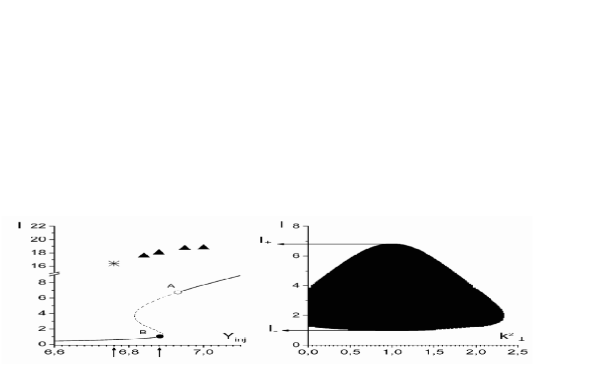
Figure 1: Right: Instability domain. Left: Steady state curve of the homogeneous solution and results of numerical simulations; continous and dashed lines refer to stable and unstable portion of the homogeneous branch, respectively. The ordinate of the asterisk and  the solid triangles symbols corrisponds respectively to the mean values of the maximum intensity $I$ of cavity light bullets and longitudinal rolls and filaments. $I_{-}$ and $I_{+}$ correspond to the minimum and the maximum intensity of the instability region and hence represent the ordinates of the limiting points $A$ and $B$ ond the stationary curve. The arrows delimit the interval of  $Y_{inj}$ where the modulated solutions coexists with the stationary homogeneous one.

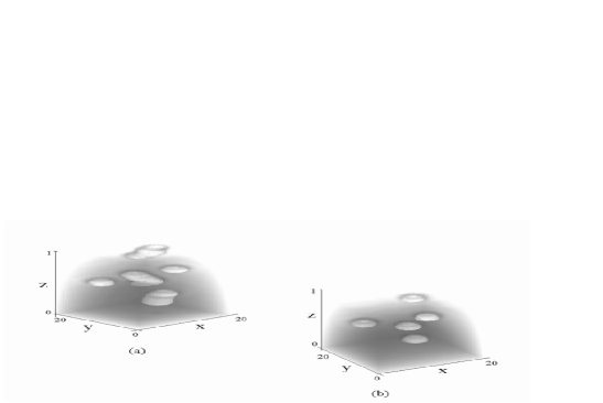
Figure 2: Example of spontaneous self-organization of the system. Gray scale isosurface of intracavity field for $Y_{inj}=6.74$. $3D$ patterns in the intensity profile (a) can collapse in localized structures (b) which make a round cavity trip in a period of $\sim L/c$. Note that in all numerical simulations the transverse spatial unit is given by the quantity $L/2k_{0}T$, while the longitudinal variable is scaled to $L$. Finally the time is scaled to the quantity $L/cT$ so that the interval between the frames represented in this figure is around $545$ time units.

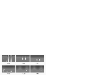
Figure 3: One transverse dimension case. Gray scale plots of intensity intracavity field profile; white represents the maximum values. (a, b, c) Sequence of frames showing the writing process of two indipendent CLBs (the whole sequence is 23 t.u. long); (d, e, f) CLB motion induced via a phase gradient in the holding beam (the whole sequence is 520 t.u. long).

References

- (1) L. A. Lugiato, M. Brambilla and A. Gatti, Advances in Atomic, Molecular and Optical Physics, 40, 229-306 (1998).
- (2) P. L. Ramazza, E. Pampaloni, S. Residori and F. T. Arecchi, Phys. D 96, 259 (1996).
- (3) S. Barland et al., Nature 419, 699 (2002).
- (4) B. Schäpers, M. Feldmann, T. Ackemann, and W. Lange, Phys. Rev. Lett. 85, 748-751 (2000).
- (5) V. B. Taranenko, K. Staliunas, and C. O. Weiss, Phys. Rev. A 56, 1582-1591 (1997).
- (6) K. Ikeda, Optics Communications 30, 257-261 (1979).
- (7) L. A. Lugiato, L. M. Narducci and M. F. Squicciarini, Phys. Rev. A 34, 3101-3108 (1986).
- (8) A. S. Patrascu et al., Optics Communications 91, 433-443 (1992).
- (9) Y. Silberberg, Opt. Lett., 15, 1282 (1990).
- (10) M. Tlidi and P. Mandel, Phys. Rev. Lett. 83, 4995-4998 (1999).
- (11) N. N. Rosanov, Opt. Spectrosc.,76, 555-557 (1994); N. N. Rosanov in Proceedings of SPIE, 4324, 102-110 (2001).
- (12) G. L. Oppo, A. J. Scroggie, and W. J. Firth, Phys. Rev. E 63, 066209 (2001).
- (13) F. Wise and P. Di Trapani, Optics and photonics news. 13, 28-32 (2002).
- (14) W. J. Firth and A. J. Scroggie, Phys. Rev. Lett. 76, 1623-1626 (1996).
- (15) L. A. Lugiato, in Progress in optics 21, 69 (1984).
- (16) M. Lax, W. H. Louisell and W. B. McKnight, Phys. Rev. A 11, 1365-1370 (1975).
- (17) Although the resulting model is not ideally suited to describe the excitonic response of a semiconductor brambilla because of its slow carrier dynamics, we can note that as far as pattern formation is involved, it has been shown in literature how the qualitative pattern and soliton scenario in the MFL saturable absorber firth2 is not radically different from the semiconductor case spinelli .
- (18) M. Brambilla et al., Phys. Rev. Lett. 79, 2042-2045 (1997).
- (19) L. Spinelli, G. Tissoni, M. Brambilla, F. Prati and L. A. Lugiato, Phys. Rev. A 58, 2542-2559 (1998).
- (20) L. A. Lugiato and C. Oldano, Phys. Rev. A 37, 3896 (1988).
- (21) L. M. Narducci et al., Phys. Rev. A 32, 1588-1595 (1985).
- (22) M. Brambilla, L. A. Lugiato and M. Stefani, Europhys. Lett. 34, 109 (1996).
- (23) L. Spinelli, M. Brambilla, The European Physical Journal D 6, 523-532 (1999).