Towards a general theory of nonlinear flow-distributed oscillations

Abstract

We outline a general theory for the analysis of flow-distributed standing and travelling wave patterns in one-dimensional, open plug-flows of oscillatory chemical media.  We treat both the amplitude and phase dynamics of small and large-amplitude waves, considering both travelling and stationary waves on an equal footing and emphasizing features that are generic to a variety of kinetic models.  We begin with a linear stability analysis for constant and periodic boundary forcing, drawing attention to the implications for systems far from a Hopf bifurcation. Among other results, we show that for systems far from a Hopf bifurcation, the first absolutely unstable mode may be a stationary wave mode.  We then introduce a non-linear formalism for studying both travelling and stationary waves and show that the wave forms and their amplitudes depend on a single reduced transport parameter.  Our formalism sheds light on cases where neither the linearized analyis nor the kinematic theory of phase waves give an adequate description, and it can be applied to study some of the more complex types of bifurcations (Canards, period-doublings, etc.) in open flow systems.

I Introduction

Among the variety of known mechanisms of spontaneous pattern formation in spatially extended chemical systems, the flow distributed oscillation (FDO) mechanism Kuznetsov -Satnoianu2001 differs from the Turing Turing and related mechanismsMuratov and from the differential flow instabilityDIFICI Toth2001 in that it does not require any differential transport of the reacting species.  The FDO mechanism, which was predictedKuznetsov Andresen physically interpreted and experimentally verifiedKaern99a -Kaern2002 , operates in open flow systems when the chemical kinetics is intrinsically oscillatory and the inflow boundary condition plays an essential role.  It is potentially relevant to biological pattern formation involving an axial growth, since an open flow system is related by a coordinate transformation to a linearly growing medium such as a plant stem or animal embryo.KMH2000a -Movebound

The governing equations of the one-dimensional open reactive flow studied are the reaction-diffusion-advection  (RDA) equation

$$\frac{\partial\mathbf{U}}{\partial t}=\mathbf{f}(\mathbf{U;}C)-v\frac{\partial\mathbf{U}}{\partial x}+D\frac{\partial^{2}\mathbf{U}}{\partial x^{2}}.$$ (1)

together with the boundary condition  $\mathbf{U}(0,t)$  at the inflow.  Here $\mathbf{U}(x,t)$ is an $N$-dimensional vector of dynamical variables (concentrations of species),  $\mathbf{f}(\mathbf{U;}C)$ is the vector-valued rate function which depends on one or more control parameters $C$, $v>0$ is the flow velocity and $D$ is the diffusion coefficient.  In general $D$ and $v$ can be matrices, allowing for differential transport, but here we focus on the case without differential transport, so that $v$ and $D$ are real scalars. We take the length of the reactor to be $L$ and impose no-flux boundary conditions at the outflow:  $\left.\partial U/\partial x\right|_{x=L}=0$.  We are interested in the case where $\mathbf{f}(\mathbf{U;}C)$ has a stable limit cycle and at least one unstable fixed point.

Insight into the physical mechanism of flow-distributed waves can be gained by considering the kinematic limit Reply of zero diffusion.  In this case equation (1) can be written as

$$\frac{d\mathbf{U}}{dt}=\mathbf{f}(\mathbf{U};C),$$ (2)

where we have introduced the advective derivative $d/dt\equiv\partial/\partial t+v\partial/\partial x$. Then the evolution of an advected fluid element is the same as that of the well-mixed system: each fluid element is an independent oscillator or batch reactor, and the inflow boundary condition serves to establish the phase of  these oscillators.Kaern99a  If the boundary condition is constant, for example, then all of the oscillators enter the reactor with the same initial phase and stationary waves result from the recurrence of the same phase at equally spaced downstream positions.  On the other hand, an oscillating boundary condition leads to upstream or downstream travelling waves, which have also been verified experimentally.KMH2000a -Satnoianu2001  While the kinematic limit is helpful for understanding the essential physics,  there are significant deviations from its predictions when diffusion becomes significant $D\neq 0.$ These deviations affect the wavelengthsComments  as well as the amplitudes and shapes of flow distributed waves.  The path in phase space of a volume element moving through the reactor may differ from that of the well-stirred system with the same initial conditions.Kaern2000  Sufficiently strong diffusion can extinguish the waves due to the diffusive mixing of adjacent fluid elements which are oscillating out of phase.

An alternative aproach to this kinematic or phase dynamics picture is the original Kuznetsov Andresen linear stability analysis which views the flow-distributed oscillations as arising from growing perturbations of an unstable uniform stationary state $\mathbf{U}(x,t)=\mathbf{U}_{0}$ where $\mathbf{U}_{0}$ is an unstable fixed point of the underlying kinetics governed by $\mathbf{f}(\mathbf{U;}C)$.  This linearized analysis is useful for predicting which small perturbations initially grow and which do not and it has been used in a variety of systems to determine thresholds for the formation of wave patterns (for example, the bifurcation from growing to evanescent stationary waves.)  However, the linearized analysis is not sufficient to determine the behavior of the waves when their amplitude becomes large.  As was pointed out in ref. Bamforth2001 , the linearized analysis is most useful when the kinetic system is not far from a supercritical Hopf bifurcation. In this case, it can give a good approximation to the wavelength of the fully developed nonlinear waves, although by itself it is inadequate to predict their amplitude or shape.  Chemical oscillators, however, have interesting dynamical regimes far from a Hopf bifurcation, showing markedly non-sinusoidal or relaxation oscillations.  In such cases, the fixed point enclosed by the limit cycle may be an unstable node rather than a focus, in which case a linearized analysis near the fixed point does not reveal the intrinsic oscillatory behavior at all.  The behavior of large perturbations can then be radically different from that of small ones.

Our goal in this work is to develop a general formalism that describes both stationary and travelling flow-distributed waves including their nonlinear behavior and deviations from the kinematic limit.  This formalism provides a unifying framework for understanding previous results and it can be applied to arbitrary kinetic models.  In contrast to previous studies of particular kinetic modelsKuznetsov Andresen Bamforth2001 Bamforth2002 , our emphasis is on generic phenomena. In particular we hope to shed light on systems with relaxation or other non-sinusoidal oscillations, where the unstable fixed point is a node rather than a focus.    In Section II we discuss the linear stability analysis of a fixed point with an emphasis on generic features of the two types of fixed points, unstable foci and unstable nodes.  We derive a general dispersion relation for small-amplitude disturbances and use it to analyze the response to time-dependent perturbations imposed at the inflow.  We show that a band of frequencies is spatially amplified, and that this band becomes narrower and sharper with increasing diffusion.  We derive general expressions for the thresholds separating absolute from convective instability as well as the threshold for extinction of stationary waves and show that the latter threshold disappears in the case of an unstable node.   If the system is far from a Hopf bifurcation, we show that, in contrast to previous examples, it is possible for sustained stationary waves to arise through an absolute instability from a transient perturbation.  In Section III we use a travelling wave ansatz to introduce a reduced one-dimensional ordinary differential equation (ODE) that describes the fully nonlinear stationary and travelling waves.  Numerical solutions of this equation are easier to obtain than those of the partial differential equation (1) and they allow us to obtain the nonlinear dispersion relation for the fully developed, large amplitude waves. A key result is that the amplitude and shape of the wave depend only on the reduced transport parameter $\Gamma\equiv D/(v-c)^{2}$ where $c$ is the phase velocity of the wave.  It is $\Gamma$ that governs the strength of deviations from the kinematic limit.  We show that in the case of relaxation oscillations these deviations are qualitatively different from those in the quasi-sinusoidal case,  and we provide a physical interpretation of the dependence on $\Gamma$.  We illustrate the application of our techniques by some numerical results.   Finally, in Section IV we summarize our conclusions and describe the prospects for applying our techniques to more complex types of bifurcations (Canards, period doublings, etc.)  in open flow systems.

Throughout the paper we use as an illustrative model the van der Pol or FitzHugh-Nagumo (FN) oscillatorMuratov FN1Dawson FN2Hagberg

$$\frac{dX}{dt} =e(X-X^{3}-Y)$$ (3)

$$\frac{dY}{dt} =-Y+10X,$$

which is described in more detail in Appendix A.  The FN model exhibits the generic features we are interested in:  it provides examples of quasi-sinusoidal oscillations changing to relaxation oscillations and an unstable focus changing to an unstable node as $e$ is increased.  Similar qualitative features occur in the Brusselator, Oregonator and other kinetic models. Appendix B describes the numerical approaches used and challenges encountered in solving the 1-D ODE described in Section III.

II Generic linearized analysis near a fixed point

In this section we pursue the approach which views flow-distributed waves as arising from instabilities of the spatially uniform solution  $\mathbf{U}(x,t)=\mathbf{U}_{0}$ of equation (1).  The systems of interest possess an unstable fixed point and a stable limit cycle.  The instability of the uniform state may be either convective or absolute.Deissler Whitham Huerre  We now consider small perturbations $\mathbf{u}(x,t)$

$$\mathbf{U}(x,t)=\mathbf{U}_{0}+\mathbf{u}(x,t).$$ (4)

of the homogeneous fixed point $\mathbf{U}_{0}.$ In the linearized approximation, $\mathbf{u}(x,t)$ obeys

$$\frac{\partial\mathbf{u}}{\partial t}=\mathbb{J}(\mathbf{U}_{0})\mathbf{u}-v\frac{\partial\mathbf{u}}{\partial x}+D\frac{\partial^{2}\mathbf{u}}{\partial x^{2}}$$ (5)

where $\mathbb{J}$ is the Jacobian matrix $\partial\mathbf{f}(\mathbf{U})/\partial\mathbf{U}.$ Let us denote the eigenvectors and eigenvalues of the Jacobian by $\mathbf{\xi}_{j}$ and $\lambda_{j}$ respectively ($j\in\{1..N\}$) and expand the perturbation $\mathbf{u}(x,t)$ in the eigenbasis as

$$\mathbf{u}(x,t)=\sum_{j=1}^{N}u_{j}(x,t)\mathbf{\xi}_{j}.$$ (6)

Substitution into the linearized equation gives a separate equation for each component:

$$\frac{\partial u_{j}}{\partial t}=\lambda_{j}u_{j}-v\frac{\partial u_{j}}{\partial x}+D\frac{\partial^{2}u_{j}}{\partial x^{2}}.$$ (7)

We are interested in the dynamics along unstable eigenvectors,  i.e., ones for which the real part of $\lambda_{j}$ is positive.  $\lambda_{j}$ may be one of a pair of complex conjugate eigenvalues $\lambda_{\pm}=\alpha\pm i\beta$ with $\alpha$ positive,  in which case $\mathbf{U}_{0}$ is an unstable focus, or it may be purely real and positive, as for an unstable node.  In general, the former case occurs in the neighborhood of a supercritical Hopf bifurcation, while the latter  may occur farther from the bifurcation.  The component equation associated with the eigenvector $\xi_{j}$ can be written as

$$\frac{\partial u_{j}}{\partial t}=(\alpha+i\beta)u_{j}-v\frac{\partial u_{j}}{\partial x}+D\frac{\partial^{2}u_{j}}{\partial x^{2}}.$$ (8)

Without loss of generality we can assume that $\beta\geqslant 0$.  The case of a purely real eigenvalue is included by setting $\beta=0$.  We seek complex exponential solutions of this equation of the form

$$u(x,t)=A\exp(i\omega t+ikx).$$ (9)

(From here on, the subscript $j$ is suppressed.)  Both $\omega$ and $k$ can be complex: $\omega=\omega_{r}+i\omega_{i}$ and $k=k_{r}+ik_{i}$.  Our sign conventions are such that positive values of $\omega_{i}$ or $k_{i}$ correspond to solutions that damp with time or downstream distance respectively.  Substitution of the complex exponential ansatz (9) into equation (8) gives the dispersion relation

$$i\omega=\alpha+i\beta-ivk-Dk^{2}.$$ (10)

We now consider modes with $\omega_{i}=0$, which represent the response to a sinusoidal forcing at the boundary with frequency $\omega_{r}.$ With this restriction to real frequencies, the real and imaginary components of the dispersion relation (10) read

$$vk_{i}+D(k_{i}^{2}-k_{r}^{2})=-\alpha,$$ (11)

$$vk_{r}+2Dk_{r}k_{i}=\beta-\omega_{r}.$$ (12)

If $\omega_{r}=\beta$ (forcing at the natural oscillation frequency), then eq. (12) can be satisfied by setting $k_{r}=0.$ Eq. (11) is then reduced to a quadratic equation in $k_{i}$, which always has a negative (spatially growing) solution provided $D/v^{2}<1/4\alpha$.  (As we will discuss below, $D/v^{2}=1/4\alpha$ marks the threshold between convective and absolute instability of the fixed point.  Beyond this threshold the dispersion relation cannot be solved with a purely real $\omega$.)  $>$$>$From this we learn that a perturbation with $\omega_{r}=\beta$ always yields a growing mode (the Hopf mode) in which the whole reactor oscillates in phase.  In fact, we shall see that $\beta$ is the midpoint of a band of amplified frequencies.  The edges of the amplified band can be derived by setting $k_{i}=0$ in eqs. (11) and (12) and solving for $\omega_{r}$.  The result is that sinusoidal perturbations are spatially amplified if

$$\beta-\sqrt{\frac{\alpha v^{2}}{D}}<\omega_{r}<\beta+\sqrt{\frac{\alpha v^{2}}{D}}$$ (13)

and they are damped otherwise.  If

$$\frac{D}{v^{2}}>\frac{\alpha}{\beta^{2}}$$ (14)

then $\omega_{r}=0$ falls outside the range of amplified frequencies and the stationary waves decay.

II.1 Threshold between Absolute and Convective Instability

An important distinction in the dynamics of open flow systems is the one between absolute and convective instability.   If a state is convectively unstable, then perturbations of the state grow in a reference frame moving with the flow velocity, but for any fixed position in the laboratory frame the disturbance eventually decays.  The effects of a perturbation of finite duration are eventually washed downstream and out of the system and the reactor returns to its initial unperturbed state.  In this case, the initial conditions at $t=0$ do not influence the asymptotic late-time behavior, which is instead controlled by the upstream boundary condition.  If a state is absolutely unstable, on the other hand, then localized perturbations grow with time at a fixed position in the laboratory frame, propagating upstream as well as downstream. This means that perturbations applied at $t=0$ continue to affect the state at late times.  From an experimental point of view,  the continuing effect of noise in the initial conditions makes an absolutely system more complicated.  Since the disturbances propagate in both directions, the system resembles a pure reaction-diffusion system where the flow plays a subordinate role. The critical slowing-down near the convective/absolute instability threshold adds to the experimental difficulty.  A convectively unstable system can be controlled more readily by manipulating the inflow boundary condition.

The distinction between the two cases can be expressed in terms of the group velocity of propagating disturbances.Andresen Bamforth2000 Whitham Huerre If there are modes with positive growth rate and upstream (negative) group velocity then the instability is absolute — otherwise, all growing disturbances are washed downstream.  The threshold between the two cases occurs when a mode with zero group velocity  $d\omega/dk=0$ has exactly zero growth with respect to time, $\omega_{i}=0$.  This represents a persistent disturbance that is not washed downstream.  From the dispersion relation (10) the condition of zero group velocity is

$$0=\frac{d\omega}{dk}=-iv-2Dk=0$$

or

$$k=\frac{-iv}{2D},$$ (15)

giving a purely imaginary wave number which can be substituted into both components of the dispersion relation (11) and (12).  The threshold for absolute instability occurs when the temporal growth rate $-\omega_{i}$ is exactly zero for this zero-group-velocity mode, so from the real component (11) we get

$$0=-\omega_{i}=\alpha-\frac{v^{2}}{2D}+D(\frac{v}{2D})^{2}=\alpha-\frac{v^{2}}{4D}$$

or

$$\frac{D}{v^{2}}=\frac{1}{4\alpha}$$ (16)

From the imaginary component (12) we get that $\omega_{r}=\beta$, which tells us that the first mode to go absolutely unstable is the Hopf mode.

Note that eq. (16)  is the same threshold mentioned above in discussing the solutions of (11) and (12).  It is the threshold beyond which the most unstable mode grows with time as well as space and therefore its frequency cannot be purely real.

II.2 Universal solutions of the dispersion relation

To illustrate the above results generically, it is helpful to express the dispersion relation in terms of dimensionless variables.  This requires a choice of a characteristic time scale.  It is convenient to use the growth time scale $\tau=1/\alpha$ and introduce the variables $\Omega\equiv\omega/\alpha$, $Q=Q_{r}+iQ_{i}\equiv vk/\alpha$, $\varepsilon\equiv D\alpha/v^{2}$ and $\Omega_{0}\equiv\beta/\alpha$.  For real $\Omega$ the two components (11) and (12) of the dispersion relation can be rewritten as

$$-Q_{i}+\varepsilon(Q_{r}^{2}-Q_{i}^{2})=1,$$ (17)

$$Q_{r}+2\varepsilon Q_{r}Q_{i}=\Omega-\Omega_{0}.$$ (18)

Numerical solutions for $Q_{r}$ and $Q_{i}$ as functions of $\Omega-\Omega_{0}$ are plotted in figure 1 for several values of $\varepsilon$.  The family of curves illustrates the qualitative features of the response to sinusoidal forcing: the band of amplified frequencies becomes becomes sharper and narrower with increasing $\varepsilon,$ and the plot of the wavenumber $Q_{r}$ versus $\Omega$ becomes more strongly nonlinear.   The maximum growth rate always occurs at $\Omega=\Omega_{0}$. The onset of absolute instability occurs when $\varepsilon=1/4$  and is marked by the appearance of a cusp in $Q_{i}$ and a vertical jump in $Q_{r}$ at $\Omega=\Omega_{0}$.  In the kinematic limit $\varepsilon\rightarrow 0$ all frequencies are amplified equally and $Q_{r}$ is a linear function of $\Omega$.

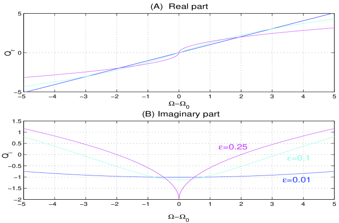
Figure 1: General solutions to the dispersion relation for small-amplitude oscillations near an unstable fixed point.  All frequencies are scaled relative to the inverse growth time scale $\alpha.$  Recall that negative values of the imaginary wavenumber $Q_{i}$ represent growing modes.  

II.3 Comments on the unstable node case

In the preceding paragraphs we have derived results for the linear stability analysis of perturbations along a single eigendirection near a fixed point of the dynamics.  The results are formally independent of whether the fixed point is a focus or a node.  The latter case can be described simply by considering $\beta=0$.   However, there are important qualitative differences between the two cases.  In the case of an unstable focus, the eigenvalues are complex conjugates and trajectories spiral away from the fixed point.  There is a single growth rate $\alpha$.  For a node, on the other hand, there is no intrinsic oscillatory behavior near the fixed point and any oscillation must be imposed externally or arise from nonlinear effects at larger amplitudes.  There are generally two eigendirections associated with distinct growth rates $\alpha_{j}$ and therefore different dispersion relations and instability thresholds for perturbations along the two eigendirections.  Perturbations grow most rapidly along the most unstable eigendirection and therefore this eigendirection is physically the most important.

Another difference between the two cases is that for a focus ($\beta\neq 0$)  the most unstable mode is always the Hopf mode which is a uniform oscillation at frequency $\beta$.  The band of amplified perturbations is centered on this nonzero frequency, which is also the first mode to become absolutely unstable. When $\beta=0,$ on the other hand, the most unstable mode (and the first to become absolutely unstable) is a stationary mode with $\omega_{r}=0.$  The linearized dispersion relation predicts a real component of the wavenumber $k_{r}=0$ for this mode.  However, when the amplitude grows, the nonlinear terms grow rapidly with the result that large-amplitude oscillation and stationary waves of finite wavelength take over.  The different nature of the absolute instability threshold between the two cases is illustrated with numerical results in figure 2.  The emergence of sustained stationary waves due to absolute instability from a time-limited perturbation (fig. 2b) is in sharp contrast to previous examplesBamforth2000 Bamforth2001  in which the first absolutely unstable mode was time-dependent (as in fig. 2a) and stationary waves in the absolutely unstable regime only occured in a thin boundary region, if at all, and only in response to a steady boundary condition held away from the fixed point.

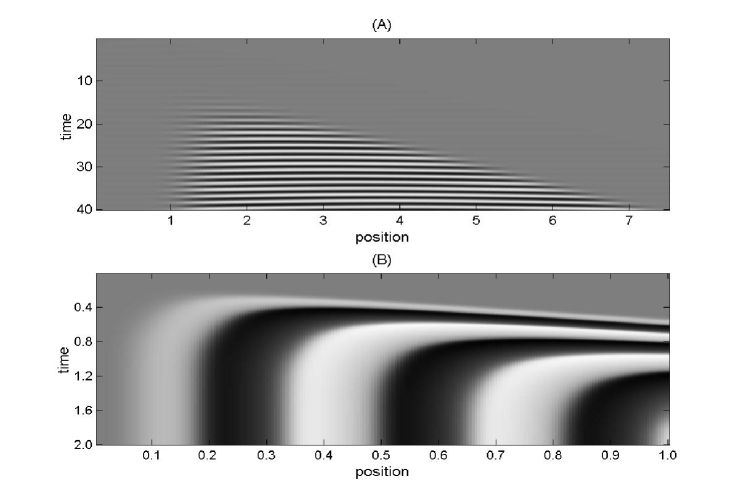
Figure 2: Onset of absolute instability in the FN system.  The gray levels are proportional to $X(x,t)$. The inflow boundary conditions are $X(0,t)=-0.001,$ $0<t<T$,  $X(0,t)=0$ otherwise, where $T=2$ in case (A), $0.1$ in case (B).  If the system were convectively unstable, the effects of the perturbation would be washed out of the system, but instead both systems are just above the threshold of absolute instability and the effects of the disturbance persist.  The pulse perturbation has a fourier spectrum of frequencies, of which the most unstable grows most rapidly.  In case (A) ($e=2$, $v=0.1,$ $D=0.0052$)  the fixed point is a focus and the first absolutely unstable mode is oscillatory.  In case (B) ($e=50,$ $v=1,$ $D=0.01$) the fixed point is a node and the first absolutely unstable mode is a stationary wave.  Although the linearized theory correctly predicts that the persistent mode is a stationary wave, it does not predict the finite wavelength, nor does it adequately describe the downstream front of the disturbance.  

II.4 Bifurcation Loci in Control Parameter Space

In a reactive flow experiment, it is typically the flow velocity which is under the experimenter’s control while the diffusion constant is fixed.  One focus of previous studies has therefore been the determination of critical flow velocities at which the FDO patterns change qualitatively.  Two important thresholds are the threshold for the formation of undamped stationary patterns $v_{T}$ and the threshold between absolute and convective instability, $v_{c},$ using the notation of ref. Andresen .  General expressions for these threshold velocities are readily obtained from (14) and (16):

$$v_{T}(C) =\frac{\beta(C)}{\sqrt{\alpha(C)}}\frac{1}{\sqrt{D}}$$ (19)

$$v_{c}(C) =2\sqrt{\alpha(C)}\frac{1}{\sqrt{D}},$$ (20)

where the dependence on kinetic control parameters $C$ has been made explicit.  These thresholds were plotted as functions of a control parameter for particular systems in refs.  Andresen ,Bamforth2000 and Bamforth2001 .  We can now understand some generic features of the shapes of these bifurcation loci observed in those works.  Near a supercritical Hopf bifurcation,  $v_{T}$ diverges and $v_{c}\rightarrow 0$ because $\alpha\rightarrow 0$.  In a range above the Hopf bifurcation, then, $v_{T}>v_{c}$ and there are three dynamical regimes as the flow velocity is varied.  At high velocities, there are sustained stationary waves which can be excited by fixed boundary conditions.  For $v_{c}<v<v_{T}$, the stationary waves are evanescent and penetrate only a limited distance into the medium.  After any initial transients are convectively washed out of the system, the remainder of the system returns to the fixed point.  Thus there is a range of $v$ values for which the unstable fixed point is effectively stabilized in the presence of constant boundary conditions.  (However, oscillatory perturbations in the amplified band still result in undamped travelling waves.)   As a control parameter is tuned farther away from the Hopf bifurcation, $\alpha(C)$ generally increases, and the two curves $v_{T}(C)$ and $v_{c}(C)$ may cross (see, for example, figure 1 of ref. Andresen ) so that for some values of $C$, $v_{T}<v_{c}$.  In this case there is no intermediate regime of evanescent waves followed by return to the fixed point as described above.  Instead, as the velocity is lowered, the absolute instability threshold is reached first.  Below $v_{c}$,  the effects of initial conditions at $t=0$ are not washed out of the system and the late-time behavior may not be controllable by the boundary condition.  The most unstable modes dominate, and stationary waves may occur only in a boundary layer with constant boundary conditions.   It is possible that the crossing of the two thresholds ($v_{T}<v_{c}$) accounts in part for the failure to observe evanescent stationary waves in experiments.Kaern99a Bamforth2001  In some cases,  as $C$ is tuned still further from a Hopf bifurcation, $\beta(C)$ may decrease to zero, and the threshold $v_{T}$ vanishes as the fixed point becomes an unstable node.  In this case, stationary waves may be triggered by an absolute instability as mentioned above.

III Nonlinear, Large Amplitude Waves

In this section we derive a reduced ordinary differential equation (ODE) that describes both stationary and travelling wave solutions of the RDA equation (1) and that applies to situations where neither the linear stability analysis nor the kinematic limit give an adequate description.  We show that the amplitude and wave form depend on a single reduced transport parameter which characterizes the degree of departure from the kinematic limit. The application of our formalism is then illustrated by some numerical examples.  As in the linearized analysis, we find that the two cases near and far from a Hopf bifurcation give qualitatively different wave behavior.

We make the ansatz $\mathbf{u}(x,t)=\mathbf{u}_{c}(x-ct)$ which is analogous to the D’Alembert solution of the wave equation.  It represents a generic wave (not necessarily periodic) travelling downstream with velocity $c$ and depending only on the combination $\zeta\equiv x-ct$.  A growing or decaying travelling wave is not strictly described by this ansatz unless $c=0$ (since a spatially changing amplitude implies a dependence on $x$ and not purely on $\zeta)$ but we expect that it describes the asymptotic behavior of such a wave when the amplitude saturates.  Substituting this into the reaction-diffusion-advection equation (1)  gives a one-dimensional ODE:

$$0=\mathbf{f}(\mathbf{u})-(v-c)\frac{\partial\mathbf{u}}{\partial\zeta}+D\frac{\partial^{2}\mathbf{u}}{\partial\zeta^{2}}.$$ (21)

With a change of variable $\zeta^{\prime}\equiv\zeta/($ $v-c)$   we obtain

$$0=\mathbf{f}(\mathbf{u})-\frac{d\mathbf{u}}{d\zeta^{\prime}}+\Gamma\frac{d^{2}\mathbf{u}}{d\zeta^{\prime 2}},$$ (22)

where $\Gamma\equiv D/(v-c)^{2}$.    $\Gamma$ represents the effective strength of the diffusion term for a given wave.  If (22) has a periodic solution $\mathbf{u}(\zeta^{\prime})=\mathbf{u}(\zeta^{\prime}+\Lambda)$, then the period $\Lambda$ in terms of $\zeta^{\prime}$ is related to the frequency and wave number of the corresponding travelling wave by

$$\omega=ck=\frac{c}{c-v}\frac{2\pi}{\Lambda(\Gamma)},$$ (23)

where we have made explicit the dependence of $\Lambda$ on $\Gamma$.

Some limiting cases are instructive and help to furnish a physical interpretation of the particular combination of parameters $\Gamma$.  First, note that the kinematic limit $\Gamma\rightarrow 0$ can be approached in several ways, either by decreasing $D$ or by increasing $\left|v-c\right|.$  The limits $c\rightarrow\pm\infty$ (infinite phase speed) both correspond to oscillations which are uniform in space.  Diffusion can have no effect on a system with no spatial gradients, and so it is understandable that the effective diffusion vanishes in this limit.  On the other hand,  as $c$ approaches $v$ from either direction $\Gamma$ diverges.  This divergence can be understood qualitatively if one considers the diffusionless limit as a “zeroth order” approximation to the phase dynamics.  In this limit, $\Lambda=\Lambda(0)$ is a constant and the physical wavelength $2\pi/k$ shrinks to zero as $c\rightarrow v$.  If a nonzero diffusion is then turned on, then it is natural to expect that it creates more mixing between crests and troughs when the waves are close together than when they are far apart.  As the wavelength shrinks, the effect of diffusion on the waveform increases.

The special case $c=0$ describes stationary waves, which result from a steady-state boundary condition.  The combination of parameters controlling the behavior of stationary waves is the same combination identified in the linearized analyisis, namely $\left.\Gamma\right|_{c=0}=D/v^{2}.$   In the case of complex eigenvalues, the condition for the existence of undamped periodic stationary waves is the one already derived using the linearized analysis:  $\Gamma<\alpha/\beta^{2}.$  Above this threshold all solutions spiral into the fixed point.  However, since the nature of solutions to (22) is governed only by $\Gamma$, one can obtain a more general threshold for undamped periodic travelling waves with phase velocity $c.$  Such waves are undamped only if

$$\Gamma=\frac{D}{(v-c)^{2}}<\frac{\alpha}{\beta^{2}}.$$ (24)

For given values of $D$ and of the kinetic control parameters that determine $\alpha$ and $\beta$,  there is an interval of phase velocities, surrounding the flow velocity, within which travelling waves do not propagate. For the case of an unstable node or $\beta=0$, on the other hand, the threshold (24) diverges and so it appears that there is no such excluded band of phase velocities.  We will further examine this issue below.

III.1 Numerical solutions and qualitative features of nonlinear waveforms

The equation (22)  is useful for several reasons.  First,  it shows that the essential features of travelling and stationary waves (the amplitude and the waveform) depend on a single combination of transport parameters, $\Gamma$ , and therefore a family of different waves are described by a single universal function.  Second, as a general rule, ODE’s can be solved with less computational effort than PDE’s, and (22)  allows one to derive wave solutions without solving the full PDE (1).   Solution methods are described in Appendix B. (22) is solved on a finite interval with boundary conditions, and the solution will in general include transients near the boundaries.  In the case $c=0$, these may represent actual transients of the stationary wave solution near the physical boundaries of the reactor.  On the other hand, if we wish to describe the asymptotic behavior of travelling wave solutions with $c\neq 0$ the transients should be ignored.

Some examples of numerical solutions for the FN system are shown in figures 3 and 4.  As expected, increasing $\Gamma$ has the general effect of increasing the deviations from the kinematic limit.  However, the behaviour differs qualitatively between the quasi-sinusoidal and the relaxation oscillation cases.  In the former case,  the phase space orbit remains approximately elliptical.  Its period remains approximately constant while its amplitude shrinks uniformly until, at the critical threshold $\Gamma=\alpha/\beta^{2}$, it vanishes into the fixed point.  In the relaxation oscillation case, on the other hand, the limit cycle does not shrink to a point. Instead, as $\Gamma$ increases, the period $\Lambda$ increases apparently without bound, and the limit cycle remains elongated in the more unstable eigendirection while narrowing in the transverse direction.

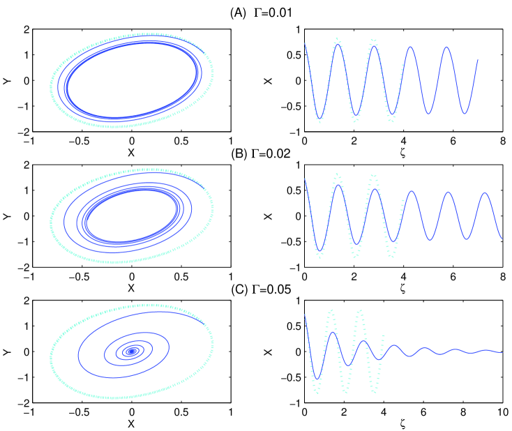
Figure 3: Numerical solutions of equation (22) for the FN system with $e=2$.  The left column shows $Y(\zeta)$ vs. $X(\zeta)$, the right shows $X(\zeta)$ vs. $\zeta$. The dotted and lighter-colored curves show solutions in the kinematic limit (or $\Gamma=0$).  The boundary conditions are fixed at a point on the local limit cycle at one end, free at the other end. For $\Gamma<0.28$ ((A) and (B))  there is a periodic quasi-sinusoidal waveform.  For $\Gamma>0.28$ (C) the solution spirals into the origin.  The period changes little as $\Gamma$ increases.  

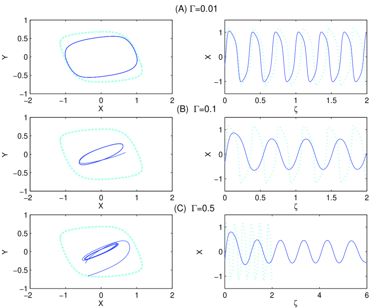
Figure 4: Solutions of equation (22) as in figure 3 but for $e=50$.  As $\Gamma$ increases, the period lengthens compared to the kinematic limit and the waveforms trace narrower loops in phase space, but they do not spiral into the origin at any finite $\Gamma$.  

III.2 “Non-linear dispersion relation”

By finding $\Lambda(\Gamma)$ numerically for a range of values of values of $\Gamma$ and then using the relation (23), one can find the non-linear dispersion relation between the frequency $\omega$ (which can be set by the forcing frequency of a perturbation at the inflow) and the phase velocity $c$ of large-amplitude travelling waves at given values of the transport parameters $D,v$. In the quasi-sinusoidal dynamical regime near the Hopf bifurcation,  $\Lambda$ is nearly constant and approximately equal to the small-amplitude oscillation period $2\pi/\beta$.   The $\omega$-$c$ relation is then approximately the same as that predicted in the kinematic limit, except that it is truncated at the cutoff frequencies $\beta\pm\sqrt{\alpha v^{2}/D\text{ }}$ where the amplitude vanishes (see figure 6B).  Outside of this interval of frequencies (which is the same as the range of amplified frequencies in the linearized theory) there are only evanescent waves.  Because of the inverse relation between $\omega$ and $v-c$, there is, as mentioned above, a range of excluded phase velocities near $v$ for which undamped travelling waves do not exist.

In the relaxation regime, on the other hand, $\Lambda$ varies quite strongly with $\Gamma.$  In fact, numerical results suggest that for asymptotically large $\Gamma$ it increases approximately linearly (see figure 5).  This means that the frequency does not become infinite as $c\rightarrow v$ but that instead there is a maximum.  Such a maximum is seen in figure 6A, which shows frequency versus phase speed for the case $e=50$, $D=0.003$, $v=1$, based on the numerical data for $\Lambda(\Gamma)$.  This relation is radically different from the one for small-amplitude, linearized waves.  The maximum frequency appears to be lower than the cutoff frequency obtained from the linear stability analysis.  There is thus a range of frequencies for which the linear theory predicts a growing mode, yet there are no large-amplitude solutions described by (22) corresponding to these frequncies.  Numerical results described below suggest that within this frequency gap the small-amplitude waves are subject to a secondary instability and do not penetrate far beyond the inflow boundary.

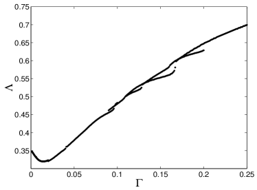
Figure 5: Scaled wavelength $\Lambda$ as a function of $\Gamma$ obtained from numerical solutions of the one-dimensional equation.  $\Lambda$ appears to increase approximately linearly for large $\Gamma$.  The numerical results become more uncertain at longer wavelengths due to the finite interval of the solution (see Appendix B).

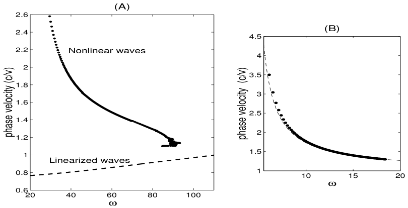
Figure 6: (A) Phase velocity vs. frequency $\omega$ for the case $e=50$, $v=1$, $D=0.003$ based on the numerical data of figure 5.  There is evidently a maximum frequency.  Perturbations near this frequency generate waves with a speed close to the flow velocity.   The phase velocity for linearized small-amplitude waves along the most unstable eigendirection is shown for comparison.  Note that the cutoff frequency for small-amplitude waves occurs precisely when their phase velocity reaches 1, as can be deduced from the dispersion relation.  The maximum frequency for large-amplitude waves (approximately $90$) appears to be lower than the linear cutoff frequency of $110$.  In the gap between these two frequencies, the linearized analysis predicts a growing mode but eq. (22) gives no solution with the correct frequency.  (B) A similar plot for $e=2,$ $v=1,$ $D=0.0025$.  In this case the phase velocity for nonlinear waves is very close to the linearized prediction, and becomes closer as the cutoff frequency of $18.36$ is approached.   

III.3 Evolution and asymptotic waveforms of growing modes

In this section we present a few numerical solutions of the PDE (1) with sinusoidal boundary forcing $(X(0,t),Y(0,t))=(a\cos\omega t,a\sin\omega t)$ where $a$ is a small perturbation amplitude ($a=0.05$ for most examples). These examples illustrate the principles discussed above, including the role of the reduced parameter $\Gamma$ and the growth of small perturbations into nonlinear waves that obey (22).  First, we illustrate the “equivalence” of waves with the same value of $\Gamma$.  Figures 7 and 8 are space-time diagrams of the FN system at $e=2$.  The diffusion constants are different, and in one case $\omega=15$ while $\omega=0$ in the other.  But in both cases $\Gamma\approx 0.006$ and so the functions $\mathbf{U}(x)$ for fixed $t$ have approximately the same shape and saturate at almost the same amplitude (slightly below the kinematic limit).

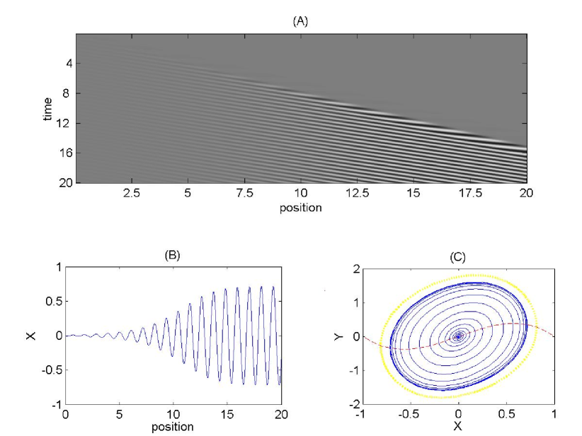
Figure 7: Growing travelling waves for $e=2$, $v=1$, $D=0.0025$ generated by a sinusoidal boundary perturbation with $\omega=15$. (A) $X(x,t)$ represented as a gray level.  (B) $X(x)$ at $t=20$.  (C) $Y(x)$ vs. $X(x)$ at $t=20$.  The limit cycle of the underlying oscillator is shown as a lighter curve, and the cubic nullcline (thin dashed line) is also shown for reference.  The actual waveform has a slightly smaller amplitude than the limit cycle of the well-stirred system.  The saturated waves have a phase velocity of 1.65, giving $\Gamma\approx 0.006$.

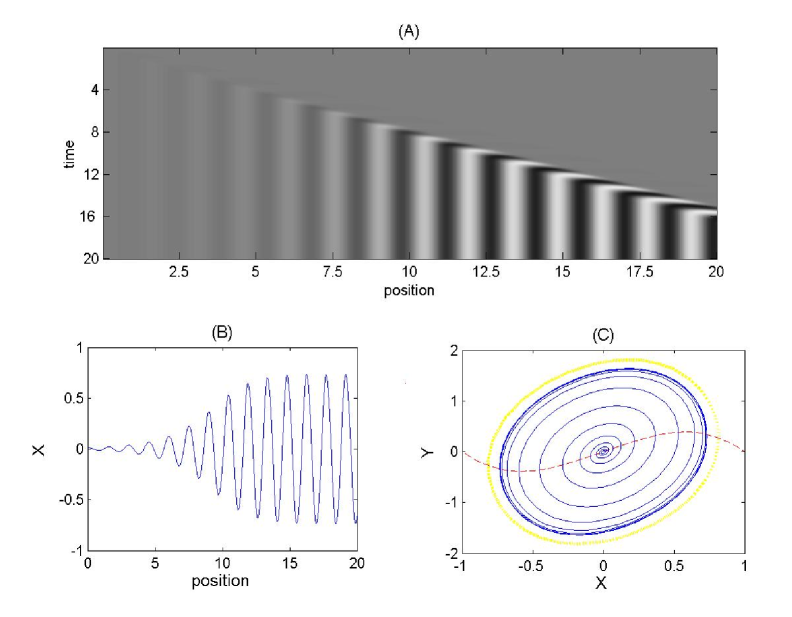
Figure 8: Stationary waves in the FN system with $e=10,$ $v=1$ and $D=0.006$ have the same value of $\mathcal{\Gamma}$ as the travelling waves in figure  7.  Their spatial waveform is similar in shape and amplitude and deviates from the kinematic limit (lighter curve) by the same amount.  

Next, we examine numerical results for $e=50$, $v=1$ and $D=0.003$, where the unstable fixed point is a node with two positive real eigenvalues.  The predicted $\omega$-$c$ relation for these parameter values is shown in figure 6A.  The boundary perturbation has components of equal size along both eigenvectors, but the component along the more unstable eigenvector of course grows faster.  Figure 9 and 10 show waves generated by perturbations with $\omega=50$ and $80$, respectively.  In both cases, the perturbation grows to a nonlinear travelling wave that deviates significantly from the kinematic limit (with more pronounced deviations in the $\omega=80$ case.)  The waveforms resemble those of figure 4.  Figure 11 shows the results of a perturbation with $\omega=85$ which is near the maximum frequency for nonlinear waves in figure 6.  In this case,  the perturbation initially grows along the more unstable eigendirection, but it penetrates only a small distance into the medium before breaking up.  Similar results were found for perturbations between $\omega\approx 85$ and the linear cutoff frequency of $\omega\approx 110$ (For $\omega>110$ the perturbations are immediately damped.)  Evidently the waves within this frequency range are subject to a secondary instability.  The patterns which arise after the high-frequency waves break up appear similar to the pulsating waves observed in refs. Kaern2000 and Kaern2002 .  The behavior of perturbations near the cutoff frequency in the case of an unstable node warrants further study.

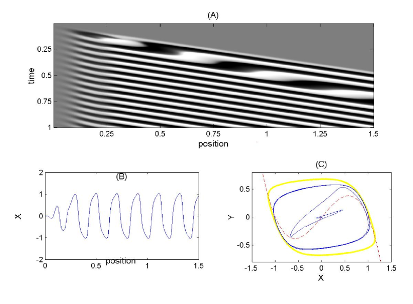
Figure 9: Waves generated by a sinusoidal perturbation with $\omega=50$ in the FN system with $e=50$, $v=1$ and $D=0.003.$  The initial transient response to the switching on of the perturbation at $t=0$ is followed by a steady travelling wave with phase velocity $c\approx 1.6$, a value consistent with the $\omega$-$c$ relation plotted in figure 6.  The corresponding value of $\Gamma$ is $0.008$ (C) shows deviations from the kinematic limit— the shape of the local orbit is shown as the broken line.  Compare (b) and (c) to figure 4a.   

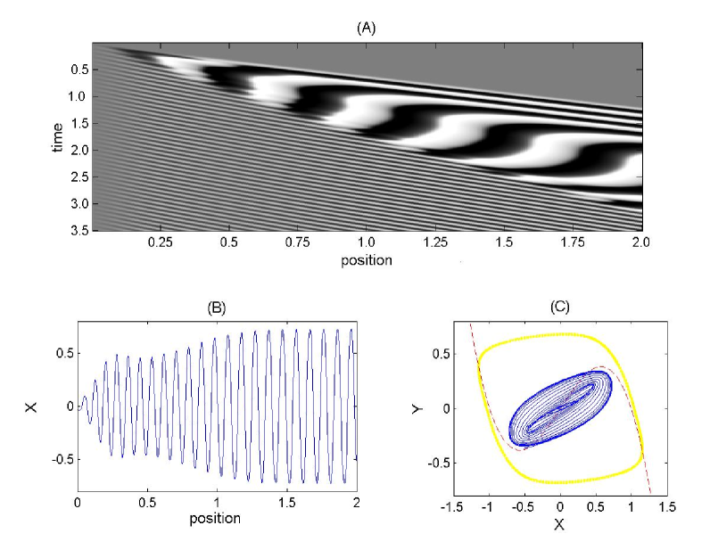
Figure 10: Waves generated by a perturbation with $\omega=80$ show a larger deviation from the kinematic limit.  The waves have $c=1.27$ and $\Gamma=0.04$.  Compare (b) and (c) with figure 4b.

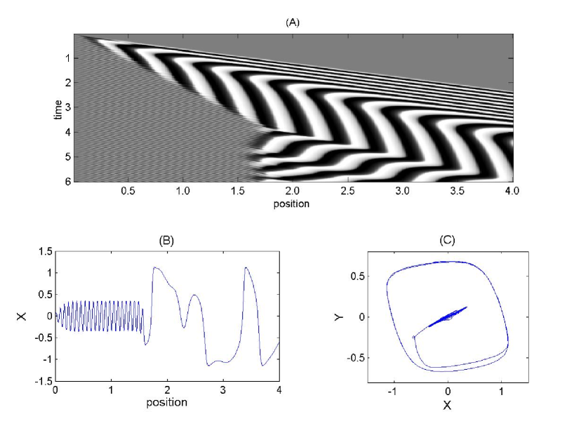
Figure 11: Boundary perturbation frequency $\omega=85$.   A high-frequency travelling wave, oscillating almost entirely along the most unstable eigendirection, penetrates a limited distance into the medium before giving way to a pattern of much longer, irregularly moving waves.  

IV Conclusions and discussion

We have attempted to give a general framework for understanding the behavior of flow-distributed waves in one-dimensional open flows of oscillatory media without differential transport, aiming at generic results.  From the point of view of linear stability analysis, we examined some changes that occur generically when an unstable fixed point changes from a focus to a node,  as typically occurs at sufficient distance from a Hopf bifurcation.  We showed that when the fixed point is a node, the first mode to become absolutely unstable is a stationary wave mode. In this case, unlike examples previously noted, a stationary wave can be established by a perturbation of finite duration in time, at least if the system is not far above the absolute instability threshold.  We derived general expressions ( eq. (13)) for the band of frequencies that result in growing waves.  The center of this band occurs at zero frequency if the unstable fixed point is a node, and at a non-zero frequency if it is a focus.  The expression for the growing frequency band allows easy calculation of the threshold for the extinction of stationary waves.  We then showed that the nonlinear behavior of periodic travelling or stationary waves reduces to a one-dimensional ODE (22) governed by the single parameter $\Gamma=D/(v-c)^{2}$, which has a physical interpretation as the strength of diffusive mixing between peaks and troughs of a particular wave.  The ODE can be solved numerically to derive the waveforms and obtain a relation between the frequency of driving at the boundary and the wavenumber and/or phase velocity of the waves generated by the perturbation.  We examined deviations of waveforms from the kinematic limit, noting qualitative differences between the quasi-harmonic and relaxation cases.

We illustrated our formalism by applying it to the FitzHugh-Nagumo toy model, but the tools we developed here can be applied to other kinetic models.  In particular, we plan to use the current results to analyze FDO patterns of complex and chaotic oscillators in a future publication.  The reduced one-dimensional equation can be applied to systems with multiple fixed points, subcritical Hopf bifurcations, Canards and bistable behavior, or other situations in which the linearized analysis gives only limited insight.

Some other questions have been left open.  The behavior of travelling waves near the cutoff frequencies in the case of an unstable node may be a fruitful subject for further study.  More generally, we have only hinted at the possibility of secondary instabilities that may affect FDO waves.  Also, in this work we have only considered regular travelling waves, not the pulsating waves observed in refs. Kaern2000 and Kaern2002 , although some of our numerical results (see figure 11)  appeared to show pulsating waves arising from a secondary instability.

V Appendix A:  The FitzHugh-Nagumo Model, quasi-sinusoidal and relaxation oscillations

The FitzHugh-Nagumo (FN) model, also known as the van der Pol oscillator,  is defined by the following pair of equationsMuratov FN1Dawson FN2Hagberg :

$$\frac{dX}{dt} =e(X-X^{3}-Y)$$ (25)

$$\frac{dY}{dt} =-Y+aX+b.$$

It is not meant to be a realistic model of any chemical system,  since its state variables include negative values, but it serves as a useful toy model that exhibits many generic features seen in real chemical systems, including bistability, excitability and ocillations of quasi-sinusoidal as well as relaxational character.

The nullclines (Fig. 12) are a cubic and a straight line. $e$ is the ratio of time scales of motion along $X$ and $Y$, $a$ is the slope of the $Y$ nullcline and $b$ is its intercept with the $Y$-axis. relaxation oscillations occur when $e$ is large.  The number and location of the fixed points depends on the  $Y$ nullcline, i.e. on values of $a$ and $b$. There may be either one fixed point or three, as shown in fig. 12.  A fixed point $(X_{\ast},Y_{\ast})$ is always stable when it lies outside the extrema of the cubic, i.e. for $X_{\ast}<-1/\sqrt{3}$ and $X_{\ast}>1/\sqrt{3}$. Depending on the parameters $(e,a,b)$ a single fixed point may be unstable and give rise to a limit cycle if $-1/\sqrt{3}<X_{\ast}<1/\sqrt{3}$.   One case that has often been studied is that of a stiff system with a large time scale separation $e\gg 1$ and a single fixed point.  In this case, as $b$ is adjusted so as to move the fixed point closer to the origin, there is first a Hopf bifurcation at a fixed point near one extremum of the cubic nullcline, and then a Canard transitionCanard in which the limit cycle changes rapidly from a small-amplitude one to a large-amplitude relaxation oscillation.  However, we do not consider the Canard transition in this paper but instead follow reference Faraday in setting $b=0$, thus ensuring a fixed point at the origin. By setting $a=10$ we also ensure that there is only one fixed point,  thus excluding bistable or excitable behavior.  In the examples we discuss, we vary only $e$.

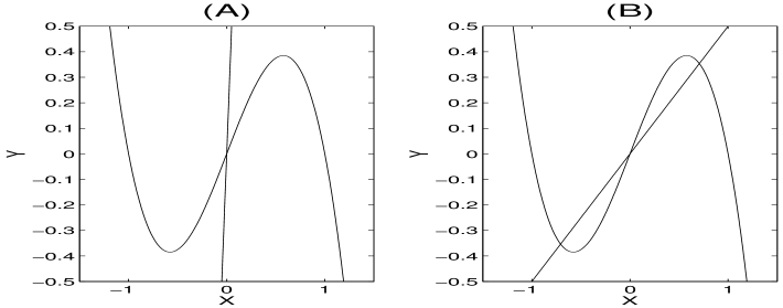
Figure 12: Nullclines for the FHN model for $b=0$ and (A) $a>1$; (B)  $a<1.$ In the latter case, there are three fixed points.

The Jacobian evaluated at the origin is given by

$$\left(\begin{array}[c]{cc}e&-e\\ a&-1\end{array}\right)$$ (26)

and its two eigenvalues are given by

$$\lambda_{\pm}=\frac{e-1}{2}\pm\frac{1}{2}\sqrt{(1+e)^{2}-4ea}.$$ (27)

The eigenvalues are complex if and only if

$$a>\frac{(1+e)^{2}}{4e}=\frac{1}{4e}+\frac{1}{2}+\frac{e}{4}.$$

Otherwise, both eigenvalues are real, and their signs are the same if $a>1$.  If the eigenvalues are complex, then their real part is positive when $e>1.$  When $a=10$, the eigenvalues are real and positive for all $e>e_{crit}\approx 38$.  Figure 13 shows the real and imaginary parts of the two eigenvalues $\lambda_{\pm}$ together with the angular frequency $\omega_{LC}=2\pi/T$ of the stable limit cycle which exists for all $e>1$.  The Hopf bifurcation occurs at $e=1$ where $\operatorname{Re}(\lambda_{\pm})$ becomes positive.  In the immediate vicinity of the Hopf bifurcation, the frequency of the limit cycle is identical to the imaginary part $\operatorname{Im}(\lambda_{+})$.  At $e_{crit}$, however,  $\operatorname{Im}(\lambda_{+})$ vanishes and the eigenvalues become real.  They are degenerate at the critical point but quickly become different as $e$ increases further.  Roughly speaking, the two real eigenvalues above $e_{crit}$ correspond to two different inverse time scales:  a slower one for motion in the $Y$ direction and a faster one for motion in the $X$ direction.  It is this separation of time scales that distinguishes relaxation oscillations from quasi-sinusoidal ones.  The frequency of relaxation oscillations is determined primarily by the slower of the two time scales.  As $e$ increases, the qualitative character of the oscillations changes from approximately sinusoidal to relaxation oscillations, as shown in figure 14.  Figure 14 shows trajectories starting from points close to the fixed point, therefore it also illustrates visually the change in character of the fixed point from an unstable focus (trajectories spiral away from the fixed point) to a node (trajectories leave along the most unstable eigenvector).  Note that although there is a sudden change in the eigenvalues and eigenvectors near the fixed point at $e_{crit}$, the associated change in the nonlinear limit cycle is gradual.

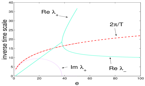
Figure 13: Inverse time scales as functions of $e$ for $a=10$.  Dotted line: $\operatorname{Im}(\lambda_{+})$;  solid lines:  $\operatorname{Re}(\lambda_{\pm})$;  dashed line:  $2\pi/T$ for the limit cycle.  At the critical value $e_{c}\approx 38$, the eigenvalues become real.  

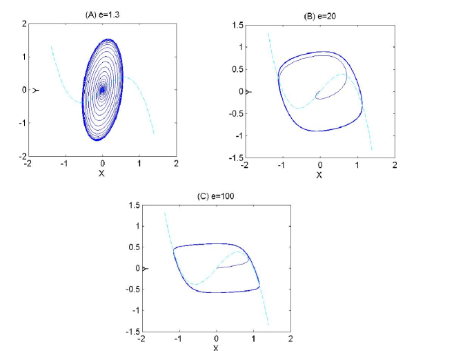
Figure 14: Trajectories of an initial condition close to the origin, for $a=10$ and three different values of $e.$ (A) $e=1.3$ is close to the Hopf bifurcation and the oscillations are quasi-sinusoidal.  (B) $e=20$ is an intermediate value, between the Hopf bifurcation and $e_{c}\approx 38$.  (C) $e=100$ is well above $e_{c}$ and the limit cycle has the character of a relaxation oscillation.   The change in the shape of the limit cycle is a gradual one, in spite of the rapid transition in the eigenvalues at the fixed point.

VI Appendix B: Numerical solutions of the reduced one-dimensional equation (22)

Here we discuss the solution of the reduced ODE (22):

$$0=\mathbf{f}(\mathbf{u})-\frac{d\mathbf{u}}{d\zeta^{\prime}}+\Gamma_{c}\frac{d^{2}\mathbf{u}}{d\zeta^{\prime 2}}.$$

In the kinematic limit $\Gamma\rightarrow 0$,  this equation reduces to a first-order equation, identical in form to that of the dynamics of the well-stirred system.  Solutions of this first-order equation with general initial conditions approach the stable limit cycle of the well-stirred system.  However, for any nonzero value of $\Gamma$ the equation is second-order and anti-dissipative, so that the initial-value problem leads to unbounded solutions for most choices of initial conditions $\mathbf{u}(0)$ and $\mathbf{u}^{\prime}(0)$.  To exclude these unphysical solutions, a boundary condition must be imposed.  Thus, the equation should be solved as a boundary-value problem on a finite interval $0<\zeta<L$.  Our procedure was to impose a fixed boundary condition on the left,  $\mathbf{u}(0)=\mathbf{u}_{in}$ and a free boundary condition on the right, $\mathbf{u}^{\prime}(0)=0$.  In the case $c=0$ the boundaries correspond directly to the the physical boundaries of the plug-flow reactor.

For the examples studied, we found that for moderate values of $\Gamma$ and for sufficiently large $L$ the solutions of the boundary problem behave qualitatively like solutions of a first-order initial value problem with an attractor.  In other words,  after some transient behavior at small $\zeta$ which depends strongly on $\mathbf{u}_{in}$,  the solutions settle either to a fixed value or to a periodic behavior with an intrinsic period $\Lambda$, which depends on $\Gamma$ but does not depend sensitively on $\mathbf{u}_{in}$ or on $L$.  The free boundary condition on the right affects the solution only in a small interval near the right boundary, i.e.,  the boundary can be moved to a larger value of $\zeta$ without changing the solution on most of the interval $0<\zeta<L$.  In the $c=0$ case, the entire solution, including the boundary transients, is physically meaningful as part of a stationary wave pattern in the reactor.  For $c\neq 0$, boundary conditions at fixed $\zeta$ values are not directly equivalent to boundary conditions at fixed $x$,  but the attractors reached by the solutions can be interpreted as the asymptotic shapes of travelling waves in the medium.

In order to obtain numerical solutions of the boundary value problem, we used a collocation algorithm included in the Matlab software package.Matlab  This algorithm requires an initial guess for the solution which is then adjusted to satisfy the differential equations and the boundary conditions within a specified tolerance.  For long solution intervals (large multiples of $\Lambda$) the algorithm may fail to converge unless the initial guess is close to the actual solution.  We used two procedures for iteratively obtaining a solution:

1. Use a solution of the initial-value problem of the first-order, $\Gamma=0$ system as an initial guess for a relatively small value of $\Gamma$.  Then increase $\Gamma$ iteratively to the desired value, using each solution as the guess for the next value of $\Gamma$.  This procedure was used, for example, to generate the solutions at a range of values of $\Gamma$ in figure 5.

2. Sometimes it is more convenient to approximate the solution with piecewise solutions on a series of overlapping intervals.  The procedure is as follows:  First,  solve the boundary value problem with the desired boundary condition $\mathbf{u}_{in}$ at $\zeta=0$ and free boundary conditions at a relatively small $L$ which is neither too much larger nor too much shorter than $\Lambda$.  Obtain a solution $\mathbf{u}_{1}(\zeta)$ on that interval.  Then evaluate that solution at $\zeta=L/2$ and use $\mathbf{u}_{1}(L/2)$ as the boundary condition for a new solution on the interval $L/2<\zeta<3L/2$.  Continue this procedure on a series of overlapping intervals.  If $L$ is not too large, then the initial trial solutions need not be close to the final ones, and if $L$ is not too small they are not sensitive to the free boundary condition at the right, so that the overlapping solutions should be approximately the same except very near the boundaries.  Stitched together, the piecewise solutions approximate a solution on a longer interval.

Large values of $\Gamma$ (where large means significantly larger than $1/4\alpha$, the threshold of absolute instability in the $c=0$ case) often presented computational challenges because the solutions become more sensitive to the right boundary condition, and large intervals were needed in order for an attractor to appear.  This is the source of some of the numerical jitter in the data in figure 5.

Acknowledgment: This work was supported by the NSERC of Canada.

References

- (1) S. P. Kuznetsov, E. Mosekilde, G. Dewel and P. Borckmanns, J. Chem. Phys. 106, 7609 (1997).
- (2) P. Andresén, M. Bache, E. Mosekilde, G. Dewel and P. Borckmanns, Phys Rev. E 60, 297 (1999).
- (3) M. Kaern and M. Menzinger, Phys. Rev. E 60, 3471 (1999).
- (4) M. Kaern and M. Menzinger, Phys. Rev. E 61, 3334 (2000).
- (5) M. Kaern and M. Menzinger, J. Phys. Chem. A 106, 4897 (2002).
- (6) P. Andresén, E. Mosekilde, G. Dewel and P. Borckmanns, Phys. Rev. E 62, 2992 (2000).
- (7) M. Kaern and M. Menzinger, Phys. Rev. E 62, 2994 (2000).
- (8) J.R. Bamforth, S. Kalliadasis, J.H. Merkin and S.K. Scott, Phys. Chem. Chem. Phys. 2, 4013 (2000).
- (9) J.R. Bamforth, J.H. Merkin, S.K. Scott, R. Tóth and V. Gáspár, Phys. Chem. Chem. Phys. 3, 1435 (2001).
- (10) J.R. Bamforth, R. Tóth, V. Gáspár and S.K. Scott, Phys. Chem. Chem. Phys. 4, 1299 (2002).
- (11) M. Kaern, M. Menzinger and A. Hunding, Biophys. Chem. 87, 121 (2000).
- (12) M. Kaern, M. Menzinger and A. Hunding, J. Theor. Biol. 207, 473 (2000).
- (13) M. Kaern, M. Menzinger, R. Satnoianu, and A. Hunding, Faraday Discussions 192, 295 (2001).
- (14) M. Kaern, R. Satnoianu, A.P. Muñuzuri and M. Menzinger, Phys. Chem. Chem. Phys. 4, 1315 (2002).
- (15) R.A. Satnoianu and M. Menzinger, Phys. Rev. E 62, 113 (2000).
- (16) R.A. Satnoianu, P.K. Maini and M. Menzinger, Physica D 160, 79 (2001).
- (17) A.M. Turing, Phil. Trans. R. Soc. London B 237, 37 (1952).
- (18) C.B. Muratov and V.V. Osipov, Phys Rev. E 54, 4860 (1996).
- (19) A.B. Rovinsky and M. Menzinger, Phys. Rev. Lett. 69, 1193 (1992); 70, 778 (1993).
- (20) R. Tóth, A. Papp, V. Gáspár, J.H. Merkin, S.K. Scott and A.F. Taylor, Phys. Chem. Chem. Phys. 3, 1435 (2001).
- (21) S.P. Dawson, M.V. D’Angelo and J.E. Pearson, Phys. Lett A 265, 346 (2000).
- (22) A. Hagberg and E. Meron, Chaos 4, 477 (1994).
- (23) R.J. Deissler, J. Stat. Phys. 40, 371 (1985); 54, 1459 (1989).
- (24) G.B. Whitham, Linear and Nonlinear Waves, Wiley, New York, 1973.
- (25) P. Huerre, in Instabilities and Nonequilibrium Structures, ed. E. Tirapegui and D. Villaroel (Reidel, 1987), 141-177.
- (26) E. Benoit, J.L. Callot, F. Diener and M. Diener, Collect. Math. 32, 37 (1981); M. Diener and T. Poston, in E. Haken, ed., Chaos and Order in Nature (Berlin, Springer-Verlag, 1981), 279-289; M. Diener, Math. Intell. 6, 38 (1984); B. Peng, V. Gaspar and K. Showalter, Phil.Trans. R. Soc. Lond. A 337, 275 (1991).
- (27) L.F. Shampine, M.W. Reichelt, and J. Kierzenka, ”Solving Boundary Value Problems for Ordinary Differential Equations in MATLAB with bvp4c,” available at ftp://ftp.mathworks.com/pub/doc/papers/bvp/.