On the parametric dependences of a class of non-linear singular maps

Abstract.

We discuss a two-parameter family of maps that generalize piecewise linear, expanding maps of the circle. One parameter measures the effect of a non-linearity which bends the branches of the linear map. The second parameter rotates points by a fixed angle. For small values of the nonlinearity parameter, we compute the invariant measure and show that it has a singular density to first order in the nonlinearity parameter. Its Fourier modes have forms similar to the Weierstrass function. We discuss the consequences of this singularity on the Lyapunov exponents and on the transport properties of the corresponding multibaker map. For larger non-linearities, the map becomes non-hyperbolic and exhibits a series of period-adding bifurcations.

T. Gilbert†‡and J. R. Dorfman†

† Department of Physics and

Institute for Physical Science and Technology

University of Maryland

College Park, MD 20742, USA

‡ Laboratoire Cassini, CNRS,

Observatoire de la Côte d’Azur

B. P. 4229, 06304 Nice, France

and

Institut Non-Linéaire de Nice

CNRS, Université de Nice

1361 Route des Lucioles, 06560 Valbonne, France

1. Introduction

The concept of natural invariant measure is central to the theory of Sinai-Ruelle-Bowen measures. Rigorous results pertaining to the existence and uniqueness of such measures have been obtained for the most part in the framework of Anosov diffeomorphisms and Axiom A systems. However, as discussed by Chernov [1], there are hyperbolic maps other than diffeomorphisms for which SRB measures were constructed [18, 22, 2]. It is our purpose to investigate some of the properties of a class of such systems with singularities.

This paper is concerned with the parametric dependence of a particularly simple class of one-dimensional circle maps which may be regarded as non-linear generalizations of a class of piece-wise linear, expanding maps. The generalized maps have two essential properties, the first being that these maps are singular in the sense that their first derivative posseses a singularity (or a finite set of them), and second that the maps perform some irrational rotation such that the singularity is moved ergodically about the circle upon iteration. This class of maps will be characterized by two parameters: a first parameter which measures the strength of the nonlinearity, and a second one which is a rotation angle.

Depending on the strength of the non-linearity, the map can be hyperbolic or be non-hyperbolic. In the framework of the one-dimensional circle maps we consider here, these two regimes are best described by measures on interval-filling attractors or by delta-measures, respectively. It is convenient to assume that the linear regime, i. e. when the non-linearity is set to zero, corresponds to a regime where the map is uniformly expanding, for instance, an angle-doubling automorphism. The onset of non-linearity perturbs this hyperbolic regime without altering this property. However, when the non-linearity reaches a threshold value, the map loses its hyperbolicity and stable periodic orbits may occur.

The presence of a rotation has interesting consequences in both these regimes. In the regime of small non-linearity, the hyperbolicity will not be affected by the rotation since the map is everywhere expanding. However, because of the existence of singularities, upon iteration, an initially uniform density will evolve into a discontinuous one. The invariant density has a dense set of discontinuities, but remains finite everywhere. For larger non-linearity, the rotation can take a non-expanding region into an expanding one, with the consequence that the attractor may alternate between hyperbolic and non-hyperbolic regions as the intensity of the non-linearity or the rotation angle are varied.

2. Singular circle maps

Consider the family of automorphisms of the circle

$$\varphi_{0,\zeta}\>:\>x\longrightarrow 2x+\zeta\mod 1\ ,$$ (1)

which combines a rotation by an angle $\zeta$ with a uniformly expanding automorphism. It is clear that the Lebesgue measure is invariant under such a map, regardless of the parameter $\zeta$. The parametric dependences of maps with a rotation become less trivial when the linear expansion is replaced by a nonlinear one. Consider maps of the form

$$\varphi_{a,\zeta}\>:\>x\longrightarrow 2f_{a}(x)+\zeta\mod 1\ ,$$ (2)

where we assume $f_{a}$ is defined over the unit interval, with the following features, motivated by previous studies of non-linear baker maps[11]  :

• the end points $0,1$ of the interval are fixed points, $f_{a}(0)=0$ and $f_{a}(1)=1$, such that the former is an attracting fixed point, $f_{a}^{\prime}(0)<1$, while the latter is repelling, $f_{a}^{\prime}(1)>1$;

• $f_{a}$ is analytic with respect to the parameter $a$;

• $f_{a}(x)$ is Holder continous with respect to the variable $x$. Moreover, all the derivatives of $f_{a}$ with respect to $x$ exist at the end points;

• $f_{a}$ has a semi-group property, namely the composition of $f_{a}$ with itself yields $f_{2a}$,

  $$f_{a}\circ f_{a}(x)=f_{2a}(x)\ ,$$ (3)

  and the inverse of $f_{a}$ is obtained by changing the sign of $a$,

  $$f_{a}^{-1}(x)=f_{-a}(x)\ ;$$ (4)

• $f_{a}$ has the following property of reversibility

  $$f_{a}(1-x)=1-f_{-a}(x)\ .$$ (5)

The semi-group property, Eqs. (3-4), imply that $f_{a}$ is the identity for $a=0$, namely $f_{0}(x)=x$;

We note that Eqs. (4-5), imply the following :

$$f_{a}^{\prime}(0)f_{a}^{\prime}(1)=1\ .$$ (6)

Moreover these quantities are different from $1$ as required in item (i).

In this paper, we will consider in its generality the class of perturbations $f_{a}$ satisfying the above properties. In particular, we will consider the small parameter regime, $|a|\ll 1$, where $f_{a}$ can be written as a power expansion in its parameter,

$$f_{a}(x)=x+af^{(1)}(x)+O(a^{2}),$$ (7)

and demand that the property of the derivative of $f_{a}$ at the extremities of the interval, see item (i) above, hold to first order in $a$.

An immediate property of $f^{(1)}$ follows from Eq. (5), namely it is symmetric with respect to $x=1/2$,

$$f^{(1)}(x)=f^{(1)}(1-x),$$ (8)

which also implies that the derivatives of $f^{(1)}$ at $x=0$ and $x=1$ have opposite slopes,

$${f^{(1)}}^{\prime}(0)=-{f^{(1)}}^{\prime}(1).$$ (9)

Therefore the perturbations $f_{a}$ under consideration have a singularity of order $a$ in their derivatives at the end points of the unit interval, which are identified by the modulo one operation.

Possible examples of such perturbations are polynomials or trigonometric functions. Such examples are

$$f_{a}(x) = x+ax(1-x)+O(a^{2})\ ,$$ (10)

$$f_{a}(x) = x-\frac{a}{\pi}\sin(\pi x)+O(a^{2})\ .$$ (11)

Figure 1. Illustration of the map $\varphi_{a,\zeta}$ defined by Eq. (2), with $f_{a}(x)$ the full form of Eq. (11) given later in Eq. (25). Here $a=1.5$ and $\zeta=0.75$.

3. Hyperbolic regime

Although $\varphi_{a,\zeta}$ is a singular map, it has a unique absolutely continuous invariant measure, provided it is everywhere expanding, that is

$$2f_{a}^{\prime}(x)>1.$$ (12)

The density of this measure has very interesting properties. Indeed, a direct consequence of the singularity of $f_{a}$ at the origin is that the iteration of a density of points initially uniform on the interval will yield a discontinuity which, provided $a$ is small, is of the order of $a$. At the next iteration this discontinuity is rotated around the circle by $\zeta.$ Further iterations yield more and more discontinuities which, as long as $\zeta$ is irrational, will cover densely the whole interval.

The invariant density is a fixed point of the Frobenius-Perron operator,

$$\rho(x)=\left\{\begin{array}[]{l@{\quad}l}\frac{1}{2}f_{-a}^{\prime}\left(\frac{x-\zeta}{2}+1\right)\rho\left[f_{-a}\left(\frac{x-\zeta}{2}+1\right)\right]\\ \\ \quad+\frac{1}{2}f_{-a}^{\prime}\left(\frac{x+1-\zeta}{2}\right)\rho\left[f_{-a}\left(\frac{x+1-\zeta}{2}\right)\right],&0\leq x<\zeta,\\ \\ \frac{1}{2}f_{-a}^{\prime}\left(\frac{x-\zeta}{2}\right)\rho\left[f_{-a}\left(\frac{x-\zeta}{2}\right)\right]\\ \\ \quad+\frac{1}{2}f_{-a}^{\prime}\left(\frac{x+1-\zeta}{2}\right)\rho\left[f_{-a}\left(\frac{x+1-\zeta}{2}\right)\right],&\zeta\leq x<1,\end{array}\right.$$ (13)

where we dropped the parametric dependences to simplify the notation.

Let us consider the first order term in the expansion of $\rho$ in $a$, namely

$$\rho(x)=1+a\rho^{(1)}(x)+O(a^{2})\ ,$$ (14)

where we have taken the uniform density, $\rho(x)=1$ to be the absolutely continuous solution of Eq. (13) when $a=0$. An expression for $\rho^{(1)}$ follows from Eq. (13) :

$$\rho^{(1)}(x)=\left\{\begin{array}[]{ll}-\frac{\displaystyle{1}}{\displaystyle{2}}{f^{(1)}}^{\prime}\left(\frac{\displaystyle{x-\zeta}}{\displaystyle{2}}+1\right)-\frac{\displaystyle{1}}{\displaystyle{2}}{f^{(1)}}^{\prime}\left(\frac{\displaystyle{x+1-\zeta}}{\displaystyle{2}}\right)&\\ \\ \quad+\frac{\displaystyle{1}}{\displaystyle{2}}\rho^{(1)}\left(\frac{\displaystyle{x-\zeta}}{\displaystyle{2}}+1\right)+\frac{\displaystyle{1}}{\displaystyle{2}}\rho^{(1)}\left(\frac{\displaystyle{x+1-\zeta}}{\displaystyle{2}}\right),&0\leq x<\zeta,\\ \\ -\frac{\displaystyle{1}}{\displaystyle{2}}{f^{(1)}}^{\prime}\left(\frac{\displaystyle{x-\zeta}}{\displaystyle{2}}\right)-\frac{\displaystyle{1}}{\displaystyle{2}}{f^{(1)}}^{\prime}\left(\frac{\displaystyle{x+1-\zeta}}{\displaystyle{2}}\right)&\\ \\ \quad+\frac{\displaystyle{1}}{\displaystyle{2}}\rho^{(1)}\left(\frac{\displaystyle{x-\zeta}}{\displaystyle{2}}\right)+\frac{\displaystyle{1}}{\displaystyle{2}}\rho^{(1)}\left(\frac{\displaystyle{x+1-\zeta}}{\displaystyle{2}}\right),&\zeta\leq x<1.\end{array}\right.$$ (15)

Let us comment here that $\rho^{(1)}$ is generally not expected to be a well-behaved function of its arguments. This is readily seen if one notices that the two RHS of Eq. (15) evaluate to different values at $x=\zeta$. This is due to the property Eq. (9) that the derivative of $f^{(1)}$ is discontinuous at the origin. Moreover the discontinuity is of order of $\delta\equiv\mathcal{O}[{f^{(1)}}^{\prime}(0)]$. Similarly, at $x=3\zeta\mod 1$ – the image of $x=\zeta$ under $\varphi_{0,\zeta}$, Eq. (1) – another discontinuity appears, this time of order $\delta/2$. In general, a discontinuity of order $\delta/2^{n}$ occurs at the $n$th iterate of $\zeta$ under $\varphi_{0,\zeta}$, i. e. at $x=(\sum_{i=0}^{n}2^{i})\zeta\mod 1$. For rational values of $\zeta$, its binary expansion is a finite series : there exists a finite integer $N$ such that $\zeta=\sum_{i=0}^{N}\omega_{i}/2^{i+1}$, $\omega_{i}\in\{0,1\}$ and $\omega_{N}=1$. In that case, after $N-1$ iterations of $\varphi_{0,\zeta}$, $\zeta$ is mapped back on one of the iterates already visited, namely the one corresponding to the next largest index $i$ for which $\omega_{i}=1$. Therefore, for rational $\zeta$’s, the set of discontinuities is finite. However this is not so for irrational $\zeta$’s. In that case, the set of discontinuities is dense, even though of exponentially small amplitudes.

Hence $\rho^{(1)}$ is a distribution, the formal expression of which can be be found by representing it as a Fourier series :

$$\rho^{(1)}(x)=\sum_{k=1}^{\infty}\left[A_{k}(\zeta)\cos(2\pi kx)+B_{k}(\zeta)\sin(2\pi kx)\right].$$ (16)

The coefficients $A_{k}(\zeta)$ and $B_{k}(\zeta)$ satisfy the recursion relations

$$A_{k}(\zeta) = -g_{k}\sin(2\pi k\zeta)+A_{2k}(\zeta)\cos(2\pi k\zeta)-B_{2k}(\zeta)\sin(2\pi k\zeta),$$

$$B_{k}(\zeta) = g_{k}\cos(2\pi k\zeta)+A_{2k}(\zeta)\sin(2\pi k\zeta)+B_{2k}(\zeta)\sin(2\pi k\zeta),$$

with solutions

$$A_{k}(\zeta) = -\sum_{n=0}^{\infty}g_{2^{n}k}\sin\left[2(2^{n+1}-1)\pi k\zeta\right],$$ (19)

$$B_{k}(\zeta) = \sum_{n=0}^{\infty}g_{2^{n}k}\cos\left[2(2^{n+1}-1)\pi k\zeta\right],$$ (20)

where

$$g_{k}=8\pi k\int_{0}^{1}dxf^{(1)}\left(\frac{x}{2}\right)\cos(2\pi kx).$$ (21)

It is not difficult to show that $g_{k}$ decays like $1/k$ for $k\gg 1$. Indeed provided all the derivatives of $f^{(1)}$ exist at $x=0$, the integral on the RHS of Eq. (21) can be written in the form of a series in $1/k^{2n}$ ($n$ integer) with bounded coefficients.

Hence the series in Eqs. (19-20) are uniformly convergent trigonometric series, so that $A_{k}$ and $B_{k}$ are both continuous functions of $\zeta$. We notice a striking similarity between the expressions of the Fourier coefficients $A_{k}$ and $B_{k}$ and Weierstrass functions [21], which are continuous, nowhere differentiable functions. As stated in Appendix A below, the fractal dimension of these functions depends on the scaling properties of the coefficients in the trigonometric series. In particular, the dimension of the graphs of $A_{k}$ and $B_{k}$ defined by Eqs. (19-20) is unity, since the coefficients in the series decay like $1/2^{n}$. Figure (2) displays the first few Fourier modes $A_{k}$ and $B_{k}$ as functions of $\zeta$, for $k=1,2,3.$ Note that modes of different $k$’s have similar shapes but decaying amplitudes as $k$ increases.

Figure 2. From top to bottom and left to right : $A_{k}(\zeta)$ for $k=1$, 2 and 3, and $B_{k}(\zeta)$ for $k=1$, 2 and 3, numerically computed from Eqs. (19-20), where $f^{(1)}$ was taken from Eq. (11)

Consider again Eq. (16), which, with the help of Eqs. (19-20), can alternatively be written in the form

$$\rho^{(1)}(x)=-\sum_{k=1}^{\infty}\sum_{n=0}^{\infty}g_{2^{n}k}\sin\left\{2\pi k\left[\left(2^{n+1}-1\right)\zeta-x\right]\right\}.$$ (22)

As we pointed out already, the dependence of $\rho^{(1)}$ upon $x$ and $\zeta$ is more complicated than the dependence of $A_{k},B_{k}$ on $\zeta$. The set of its discontinuities is dense with respect to both arguments, even though $\rho^{(1)}$ takes finite values everywhere. Nevertheless, the explicit formal functional form allows us to calculate some quantities of interest which involve $\rho^{(1)}$ only under the integration sign. Such quantities are related to the Lyapunov exponent of the map and the transport properties of the same map “lifted” onto the real line. This is the subject of the next section.

4. Lyapunov exponents and transport properties

The positive Lyapunov exponent can be computed up to second order in $a$ with the help of Eqs. (14,16) :

$$\lambda_{+}(a,\zeta) = \int_{0}^{1}dx\rho(x)\log\left[\left|\frac{d\varphi_{a,\zeta}(x)}{dx}\right|\right]$$

$$= \log(2)-a^{2}\left(\frac{\displaystyle{1}}{\displaystyle{4}}+\frac{\displaystyle{4}}{\displaystyle{\pi}}\sum_{k=1}^{\infty}\frac{\displaystyle{kB_{k}(\zeta)}}{\displaystyle{4k^{2}-1}}\right)+O(a^{4}).$$

With the expression of $B_{k}(\zeta)$ given by Eq. (20), the summation in the last line can easily be computed numerically.

Figure 3. Absolute value of the second order correction to $\lambda_{+}(a,\zeta)$, Eq. (4). Here and in the next figure, $g$ is derived from Eq. (11).

Figure (3) shows the second order correction to $\lambda_{+}$ as a function of $\zeta.$ The fact that it is a symmetric function with respect to $\zeta\rightarrow 1-\zeta$ is a consequence of a symmetry of the map under $\zeta\rightarrow 1-\zeta,\>a\rightarrow-a,\>x\rightarrow 1-x$ and the fact that the positive Lyapunov exponent is a function only of the even powers of $a.$

The stationary drift velocity measures the exchange of particles between the unit cells of the periodically extended version of $\varphi_{a,\zeta}$. In this extension, based on the multi-baker map, points are sent to corresponding points in the unit intervals to their right and left after each iteration of the map. Points in the interval $(f_{a}((1-\zeta)/2),f_{a}((2-\zeta)/2))$, mod$(1)$, are sent one unit interval to the right, and assigned a velocity $v=+1$, while the remaining points in the interval $(0,1)$ are sent one unit to the left and assigned a velocity $v=-1$, with identical behavior in each unit interval of the real line. This is, in fact, the projection onto the $x$-axis of the nonlinear multi-baker map described in Appendix B (see Eq. (35)). The expression for the stationary drift is now straightforward and yields

$$v(a,\zeta) = -\int_{0}^{f_{-a}((1-\zeta)/2)}dx\rho(x)$$ (24)

$$+\int_{f_{-a}((1-\zeta)/2)}^{f_{-a}((2-\zeta)/2)}dx\rho(x)-\int_{f_{-a}((2-\zeta)/2)}^{1}dx\rho(x).$$

$$= -\frac{\displaystyle{2a}}{\displaystyle{\pi}}\Big{\{}\cos\left(\frac{\displaystyle{\pi\zeta}}{\displaystyle{2}}\right)-\sin\left(\frac{\displaystyle{\pi\zeta}}{\displaystyle{2}}\right)$$

$$+\sum_{k\>{\rm odd}}\sum_{n=0}^{\infty}\frac{\displaystyle{g_{2^{n}k}}}{\displaystyle{k}}\cos\left[\left(2^{n+2}-1\right)\pi k\zeta\right]\Big{\}}+O(a^{3}),$$

Its graph is displayed in Fig. (4). The drift velocity is an odd function of $\zeta-1/2$. An interesting feature of Fig. (4) is that the drift velocity is negative in a small interval about $\zeta=1/2.$ This is another example of the negative current phenomenon discovered by Groeneveld in one dimensional maps, and discussed by Groeneveld, Klages, and coworkers [12, 14, 10], and it loosely corresponds to a negative electrical conductivity, where the current is in a direction opposite to that of the electric field, taken to be in the direction of $\zeta-1/2$.

Figure 4. Drift velocity to first order in $a$, Eq. (24).

In Appendix B we present a generalization of our one-dimensional maps to two-dimensional maps, known as multi-baker maps. These maps have both a positive and a negative Lyapunov exponent. We believe that their sum obeys an identity relating the phase space contraction rate to the drift velocity, and is given as Eq. (38). We do not yet have a rigorous proof of this identity, however.

5. Non hyperbolic regime

Next, we describe some of the interesting features of the map $\varphi_{a,\zeta}$ for higher values of the field parameter. In Appendix C, we present a classification of the non-linear maps $f_{a}$ satisfying the conditions listed in Sec. 2. We will restrict our attention to $f_{a}$ given by

$$f_{a}(x)=\frac{\displaystyle{2}}{\displaystyle{\pi}}\arctan\left[\tan\left(\frac{\displaystyle{\pi x}}{\displaystyle{2}}\right)e^{-a}\right],$$ (25)

which is derived in Appendix B. As was mentioned in [11], for $\zeta=0,$ the map loses its hyperbolicity for $a>a_{c}=\log(2)$ and the origin becomes an attractive fixed point of the reduced map, so that, on a periodic lattice, the stationary state motion of particles is ballistic and moves toward decreasing $n$’s.

Things change quite dramatically as $\zeta$ is increased. The origin is now mapped to $\zeta$ and, for $\zeta$ large enough, the orbit of the origin can eventually become hyperbolic, even though the slope of $\varphi_{a,\zeta}$ at $x=0$ would be less than one. The fixed point is not the origin $x=0$ anymore and it becomes attractive for larger and larger values of $a$ as one increases $\zeta,$ i. e. $a_{c}(\zeta),$ the value of the field parameter at which the fixed point becomes attractive, is a monotonically increasing function of $\zeta.$

Moreover, for fixed $\zeta$, stable periodic orbits can be observed in the range of $a$ between $\log(2)$ and $a_{c},$ as shown in Fig. (5). A property of these windows is that they all have $0$ as a fixed point for the value of $a$ right before they bifurcate to chaotic windows. Based on this observation, it is possible to work out a condition for the presence of a window of stable period $n$ trajectories, namely that

$$\varphi_{a,\zeta}^{n}(0) = 0,$$

$$\left.\frac{\displaystyle{d}}{\displaystyle{dx}}\varphi_{a,\zeta}^{n}(x)\right|_{x=0} \leq 1,$$ (26)

where the superscript $n$ denotes the $n_{\rm th}$ iterate. The system Eq. (26) can be studied in order to find the minimal value of $\zeta$ for which there exists such a stable period $n$ orbit and the corresponding value of $a$ at which it occurs.

We illustrate this procedure for the simplest case of $n=2.$ From the top line of Eq. (26), we find

$$e^{a}=\frac{\displaystyle{2\tan(\pi\zeta/4)}}{\displaystyle{[1-\tan(\pi\zeta/4)]^{2}}},$$ (27)

while the bottom line gives

$$e^{a}\geq\frac{\displaystyle{7+\cos(\pi\zeta)}}{\displaystyle{1+\cos(\pi\zeta)}}.$$ (28)

The minimal value of $\zeta$ satisfying Eqs. (27, 28) is $\zeta\simeq 0.522873,$ for which $a\simeq 1.005053.$ The existence of this periodic orbit is confirmed numerically.

Higher $n$’s are found to start appearing at lower values of $\zeta,$ which means that, for a fixed $\zeta,$ all the periods $n$ greater than the first existing one will appear and they do so as $a$ increases until it reaches its critical value $a_{c}.$ Such a succession of stable periodic windows with increasing periods is referred to as a period adding-bifurcation, [15]. Here stable periodic windows alternate with chaotic ones. The similarity of the bifurcations observed here with period-adding bifurcations of reversible circle maps can be explained qualitatively if one notices that the two branches of $\varphi_{a,\zeta}$ have very different widths. Indeed the first critical point $x=f_{a}(1/2)$ gets closer to $x=1$ as $a$ increases, so that the first branch is close to a reversible circle map, whereas the second branch has a very steep slope. In this sense, for a fixed large $a$, as we vary $\zeta$, we expect to see periodic orbits that remain on the first branch and thus correspond to stable windows, while the second branch accounts for the chaotic windows separating stable periodic windows.

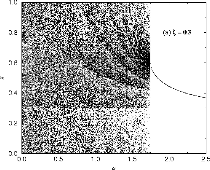
Figure 5. The bifurcation diagrams of $\varphi_{a,\zeta}(x)$ for $\zeta=0.3$ as a function of $a$.

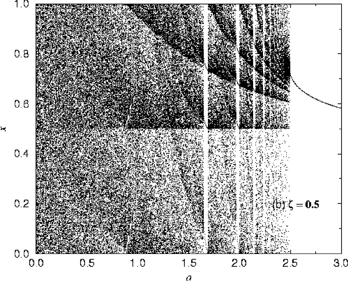
Figure 6. Same as in Fig. (5) for $\zeta=0.5.$

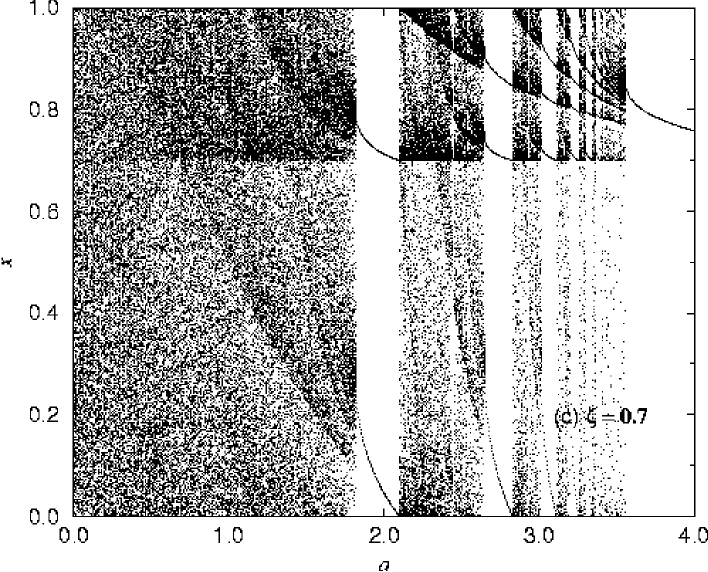
Figure 7. Same as in Fig. (5) for $\zeta=0.7.$

We illustrate this in Figs. (5-7) for the case of $\zeta=0.3,$ 0.5, and 0.7. In the first example, $\zeta=0.3,$ stable periodic windows are barely visible but one can check the existence of a period 6 window at $a\simeq 1.4449$ whose width is $O(10^{-4}).$ As $\zeta$ is increased to 0.5, windows get larger and, at $a=1.6492$ a period $3$ window starts that ends at $a=1.6881,$ then a period $4$ window arises at $a=1.9678$ that ends at $a=1.9985,$ and so on. But this is not the end of the story : besides the main sequence, there are a number of subsequences, such as $2n+1,$ $3n+1,$ $3n+2,$ etc., some of which are clearly distinguishable on the third example, $\zeta=0.7.$ The higher $\zeta,$ the greater the number of such subsequences.

6. Conclusions and Discussion

In this paper we considered a class of two-parameter singular circle maps. One of these two parameters, denoted $a$, measures the intensity of the non-linearity. In the generalization of the non-linear baker map considered in Appendix B, it plays the role of a thermostatted electric field. The other parameter, denoted $\zeta$, represents an external field, similar in some ways to a magnetic field. We found that the map exhibits both hyperbolic and non-hyperbolic behaviors, and that for small non-linearities, we could determine analytically the SRB measure of the fractal attractor to first order in $a$ and the first non zero correction, of order $a^{2},$ to the positive Lyapunov exponent. For large enough $a$ we observed a transition to non-hyperbolic behavior with a period-adding bifurcation sequence leading to a stable fixed point for large enough $a$.

Thus, the rotation parameter leads to a much more complicated dynamical behavior of the map, including a region of “negative currents” similar to those found before by Groeneveld, Klages, and coworkers [12, 14, 10].

The results of this paper lead us to the following observation : The dynamical systems studied here are, in their hyperbolic regions, not Anosov diffeomorphisms. We find that the SRB measure of the fractal attractor is not a differentiable function of the parameter $\zeta$, as it would be if the map were an Anosov diffeomorphism (i. e. did not have a singularity) [19, 7]. Instead, it is a singular function of that parameter. As hyperbolic systems which are not Anosov occur frequently in models of physical systems [6] it is not unreasonable to suppose that there will exist situations where non-differentiable SRB measures occur in physical systems. Our work suggests, at least, that this might very well be the case in Lorentz gases or other discontinuous systems in the presence of external fields, where singularities of the flow would be rotated as the field is varied.

Appendix A Weierstrass function

For $\lambda>1$ and $1<s<2$, the Weierstrass function [21] can be defined as

$$W_{\lambda,s}\>:\>[0,1]\longrightarrow\mathbf{R},\quad t\longrightarrow\sum_{k=1}^{\infty}\lambda^{(s-2)k}\sin(\lambda^{k}t)\ .$$ (29)

It is a nowhere differentiable continuous function [13].

As stated by Falconer [5], provided $\lambda$ is large enough, the box counting dimension of the graph of this function is

$$\mbox{dim}_{B}{\mathcal{G}}(W_{\lambda,s})=s\ .$$ (30)

In general, the function

$$F_{\lambda,s}(t)=\sum_{k=1}^{\infty}\lambda^{(s-2)k}g(\lambda^{k}t)$$ (31)

has box counting dimension $s$. This constitutes an upper bound for the Hausdorff dimension. However, it is commonly believed [3] that the Hausdorff dimension is exactly equal to $s$.

The case $s=1$, which is relevant to the Fourier modes given by Eqs. (19-20), is borderline. In this case, despite the nowhere differentiability of the Weierstrass function, it is understood that its Hausdorff dimension is equal to 1 [4, 17].

Appendix B Non-linear baker maps

Motivated by the analytical study of non-equilibrium stationary states of thermostated field driven systems, Gilbert et al. introduced in [11] the one parameter family of maps

$$M_{a}(n,x,y)=({\bf 1},{\bf 1},f_{a})\circ M_{0}\circ({\bf 1},f_{a},{\bf 1})\>(n,x,y),$$ (32)

where ${\bf 1}$ denotes the identity operator, acting either on integers or on points of the unit circle, $M_{0}$ is the usual multi-baker map [8, 20, 9],

$$M_{0}(n,x,y)=\left\{\begin{array}[]{l@{\quad}l}(n-1,2x,\frac{\displaystyle{y}}{\displaystyle{2}}),&0\leq x<\frac{1}{2},\\ (n+1,2x-1,\frac{\displaystyle{y+1}}{\displaystyle{2}}),&\quad\frac{1}{2}\leq x<1,\end{array}\right.$$ (33)

with variables $n\in{\bf Z}$ and $(x,y)\in[0,1]^{2}$. Here $f_{a}$ is a non-linear perturbation of the unit interval onto itself, which models the action of a thermostated external field,

$$f_{a}(x)=\frac{\displaystyle{2}}{\displaystyle{\pi}}\arctan\left[\tan\left(\frac{\displaystyle{\pi x}}{\displaystyle{2}}\right)e^{-a}\right].$$ (34)

This model is a caricature of the two-dimensional periodic thermostated Lorentz gas with an applied electric field [16] Here the variable $\pi x$ plays the role of the angle that the velocity makes with the direction of the electric field.

We generalize Eq. (32) by introducing, in the multi-baker map, Eq. (33), a new parameter, $\zeta,$ defined modulo 1, acting on the unit square, which shifts points by an angle $\zeta$ in the $x$-direction and acts on the $y$-direction so as to guarantee a weakened form of reversibility, see Eq. (36) below.

The new multi-baker map, Fig. (8), constructed so as to reduce to the multi-baker map, Eq. (33), for $\zeta=0$ and $1$, reads :

$$M_{0,\zeta}(n,x,y)=\left\{\begin{array}[]{l@{\quad}l}(n-1,2x+\zeta,\frac{\displaystyle{y+2-\zeta}}{\displaystyle{2}}),&0\leq x<\frac{\displaystyle{1-\zeta}}{\displaystyle{2}},\\ &\quad 0\leq y<\zeta,\\ (n-1,2x+\zeta,\frac{\displaystyle{y-\zeta}}{\displaystyle{2}}),&0\leq x<\frac{\displaystyle{1-\zeta}}{\displaystyle{2}},\\ &\quad\zeta\leq y<1,\\ (n+1,2x+\zeta-1,\frac{\displaystyle{y+1-\zeta}}{\displaystyle{2}}),&\frac{\displaystyle{1-\zeta}}{\displaystyle{2}}\leq x<\frac{\displaystyle{2-\zeta}}{\displaystyle{2}},\\ &\quad\>0\leq y<1,\\ (n-1,2x+\zeta-2,\frac{\displaystyle{y+2-\zeta}}{\displaystyle{2}}),&\frac{\displaystyle{2-\zeta}}{\displaystyle{2}}\leq x<1,\\ &\quad 0\leq y<\zeta,\\ (n-1,2x+\zeta-2,\frac{\displaystyle{y-\zeta}}{\displaystyle{2}}),&\frac{\displaystyle{2-\zeta}}{\displaystyle{2}}\leq x<1,\\ &\quad\zeta\leq y<1.\\ \end{array}\right.$$ (35)

Figure 8. $M_{0,\zeta}$ for $\zeta=0.25.$

The action of the time reversal operator $T,$ $T(x,y)=(1-y,1-x),$ on this map can be seen to give

$$T\circ M_{0,\zeta}\circ T=M_{0,1-\zeta}^{-1}.$$ (36)

Thus, under time reversal, the map (35) becomes the inverse of $M_{0,1-\zeta}$ instead of the inverse of $M_{0,\zeta}$. This property is reminiscent of the effect of time reversal on an external magnetic field, which changes the sign of the field.

We now define the two parameter map $M_{a,\zeta}(n,x,y),$ the same way as $M_{a}$ in Eq. (32), by

$$M_{a,\zeta}(n,x,y)=({\bf 1},{\bf 1},f_{a})\circ M_{0,\zeta}\circ({\bf 1},f_{a},{\bf 1})\>(n,x,y),$$ (37)

Despite the lack of a precise reversibility, it is interesting to ask whether the the usual result relating the irreversible entropy production to the sum of the Lyapunov exponents still holds :

$$\frac{\displaystyle{{\overline{v}}^{2}}}{\displaystyle{D}}=-(\lambda_{+}+\lambda_{-}).$$ (38)

We believe it is the case here. This view is motivated by the symmetries present. However a definite answer based upon rigorous arguments has yet to be reached.

Appendix C Classification of time-reversible perturbations

In this appendix we present a classification of the perturbations $f_{a}(x)$, with fixed points at $x=0$ and $x=1$, that satisfy the time-reversibility properties, Eqs. (3-5). In order to find explicit forms of perturbations, it is natural to assume factorizability of the $x$ and $a$ dependences. Thus consider the two classes

$$f_{a}(x) = g^{-1}\circ[g(x)q(a)]\ ,$$ (39)

$$f_{a}(x) = h^{-1}\circ[h(x)+r(a)]\ .$$ (40)

Here the parameter functions $q$ and $r$ are any functions of $a$ with the respective properties,

$$q(0) = 1\ ,$$ (41)

$$q(a)^{n} = q(na),$$ (42)

$$q(a)q(-a) = 1\ ,$$ (43)

$$r(0) = 0\ ,$$ (44)

$$nr(a) = r(na)\ ,$$ (45)

$$r(a)+r(-a) = 0\ ,$$ (46)

where $n$ is a positive integer. In particular these conditions imply the property Eq. (4) for $f_{a}$. We note that any function $r$ of the second class defines a function $q$ of the first class by exponentiation, $q(a)=\exp[r(a)]$. The only function $r$ satisfying Eqs. (44-46) is a linear function $r(a)=ca$, where $c$ is an arbitrary constant that can be taken to be $c=-1$ without loss of generality, since $a$ is allowed to take any real value. Likewise $q(a)=\exp(-a)$ is the only function that needs to be considered.

The reversal symmetry, Eq. (5), is satisfied provided

$$1-g^{-1}\circ[g(x)q(a)] = g^{-1}\circ[g(1-x)/q(a)]\ ,$$ (47)

$$1-h^{-1}\circ[h(x)+r(a)] = h^{-1}\circ[h(1-x)-r(a)]\ .$$ (48)

A class of functions verifying Eq. (47) is the set of functions $g$ with the properties

$$g(x) = \frac{1}{g(1-x)},$$ (49)

$$g^{-1}(x) = 1-g^{-1}\big{(}\frac{1}{x}\big{)}\ ,$$ (50)

Notice that the requirement that $x=0$,$1$ be fixed points of $f_{a}$ implies that $g$ is either zero or plus or minus infinity at these points. Such examples are $g(x)=\tan(\pi x/2)$, $\cot(\pi x/2)$, which define identical $f_{a}$’s up to a change of sign of $a$.

Similarly a class of functions verifying Eq. (48) is defined by

$$h(x) = -h(1-x)\ ,$$ (51)

$$h^{-1}(x) = 1-h^{-1}(-x)\ ,$$ (52)

examples of which are $h(x)=\cot(\pi x)$, $\cos(\pi x)$. Note however that $\cos(\pi x)$ is not consistent with the requirement that $x=0$, $1$ remain fixed points of $f_{a}$. Moreover the choice $\cot(\pi x)$ yields a perturbation $f_{a}$ with smooth derivative at the origin, $f_{a}^{\prime}(0)=f_{a}^{\prime}(1)=1$. This can be easily seen to yield a differentiable density $\rho^{(1)}$.

We therefore argue that the choice of $f_{a}$ given by Eq. (25) is generic. Other forms of perturbations such as polynomial in powers of $a$ can be constructed, but they do not have a complete form and can only be considered for values of $a$ small enough with respect to the degree of the polynomial approximation. Thus the non-hyperbolic regime, where $a$ becomes large, can only be studied with the example given in Sec. 5.

References

- [1] N. Chernov, Invariant measures for hyperbolic dynamical systems, in: Handbook of Dynamical Systems, A. Katok and B. Hasselblatt, ed., Elsevier, 2002
- [2] E. Catsigeras, and H. Enrich, SRB measures of certain almost hyperbolic diffeomorphisms with a tangency, Discrete Cont. Dyn. S., 7 (2001) 177–202.
- [3] G. A. Edgar, Classics on Fractals, Addison-Wesley, Reading, MA, 1993.
- [4] G. A. Edgar, private communication.
- [5] K. J. Falconer, Fractal Geometry, Wiley, New York, 1990.
- [6] G. Gallavotti and E. G. D. Cohen, Dynamical ensembles and nonequilibrium statistical mechanics, Phys. Rev. Lett., 74 (1995) 2694–2697.
- [7] G. Gallavotti and D. Ruelle, SRB states and nonequilibrium statistical mechanics close to equilibrium, Comm. Math. Phys., 190 (1997) 279–285.
- [8] P. Gaspard, Diffusion, effusion, and chaotic scattering: An exactly solvable Liouvillian dynamics, J. Stat. Phys., 68 (1992) 673–747.
- [9] P. Gaspard, Chaos, Scattering, and Statistical Mechanics, Cambridge University Press, Cambridge, 1998.
- [10] P. Gaspard and R. Klages, Chaotic and fractal properties of deterministic diffusion-reaction processes, Chaos, 8 (1998) 409–423.
- [11] T. Gilbert, C. D. Ferguson, and J. R. Dorfman, Field driven thermostated system : a non-linear multi baker map, Phys. Rev. E, 59 (1999) 364–371.
- [12] J. Groeneveld and R. Klages, Negative and nonlinear response in an exactly solved dynamical model of particle transport, J. Stat. Phys. 109 (2002), 821–861.
- [13] G. H. Hardy, Weierstrass’ non-differentiable function, Trans. Amer. Math. Soc., 17 (1916) 301–325.
- [14] R. Klages and J. Groeneveld, Einfache deterministische dynamische Systeme mit Drift: negative Stromst rken und Unterdrückung von Diffusion Verhandl. DPG (VI), 33 (1998) 646.
- [15] M. Levi, A period-adding phenomenon, SIAM J. Appl. Math., 50 (1990) 943–955.
- [16] J. Lloyd, N. Niemeyer, L. Rondoni, and G. P. Morriss, The nonequilibrium Lorentz gas, Chaos, 5 (1995) 536–551.
- [17] R. D. Mauldin and L. Pitt, private communication.
- [18] Ya. B. Pesin, Dynamical systems with generalized hyperbolic attractors, Ergod. Th. Dynam. Sys., 12 (1992) 123–151.
- [19] D. Ruelle, Differentiation of SRB states, Comm. Math. Phys., 187 (1997) 227–241.
- [20] S. Tasaki and P. Gaspard, Fick’s law and fractality of nonequilibrium stationary states in a reversible multibaker map, J. Stat. Phys., 81 (1995) 935–987.
- [21] K. Weierstrass, über continuierliche functionen eines reellen arguments, die für keinen werth des letzteren einen bestimmten differentialquotienten besitzen, In K. Weierstrass Mathematische Werke, Mayer and Müller, Berlin, 1895.
- [22] L.-S. Young, Statistical properties of dynamical systems with some hyperbolicity, Annals of Math., 147 (1998), 585–650.