Global well-posedness and multi-tone solutions of a class of nonlinear nonlocal cochlear models in hearing

Abstract

We study a class of nonlinear nonlocal cochlear models of the transmission line type, describing the motion of basilar membrane (BM) in the cochlea. They are damped dispersive partial differential equations (PDEs) driven by time dependent boundary forcing due to the input sounds. The global well-posedness in time follows from energy estimates. Uniform bounds of solutions hold in case of bounded nonlinear damping. When the input sounds are multi-frequency tones, and the nonlinearity in the PDEs is cubic, we construct smooth quasi-periodic solutions (multi-tone solutions) in the weakly nonlinear regime, where new frequencies are generated due to nonlinear interaction. When the input is two tones at frequencies $f_{1}$, $f_{2}$ ($f_{1}<f_{2}$), and high enough intensities, numerical results illustrate the formation of combination tones at $2f_{1}-f_{2}$ and $2f_{2}-f_{1}$, in agreement with hearing experiments. We visualize the frequency content of solutions through the FFT power spectral density of displacement at selected spatial locations on BM.

1 Introduction

Digital signal processing on sounds is an essential component of modern hearing devices [16], and a useful tool for evaluating acoustic theories of peripheral auditory systems, [13] among others. A fundamental issue is to model the auditory response to complex tones because the nonlinear interaction of acoustic waves of different frequencies allows for audio compression [16] among other applications. Nonlinearities are known to originate in the cochlea and are further modified in higher level auditory pathways. The cochlear mechanics has first principle descriptions, and so partial differential equations (PDEs) become a natural mathematical framework to initiate computation. However, in vivo cochlear dynamics is not a pure mechanical problem, and neural couplings are present to modify responses. To incorporate both aspects, a first-principle based PDE model was studied in [21] for voice signal processing, where the neural aspect is introduced in the model phenomenologically. The first principle based PDE approach is more systematic compared with filter bank method [13], and has shown encouraging results. In [21], time domain computation on multi-tone inputs revealed tonal suppressions in qualitative agreement with earlier neural experimental findings.

In this paper, we shall analyze the well-posedness and construct multitone solutions of such PDE models in the form:

$$p_{xx}-Nu_{tt}=\epsilon_{s}(x)u_{t},\;\;x\in(0,L),$$ (1.1)

$$p=mu_{tt}+r(x,|u|,|u_{t}|)u_{t}+s(x)u,$$ (1.2)

where $p$ is the fluid pressure difference across the basilar membrane (BM), $u$ the BM displacement, $L$ the longitudinal length of BM; $N$ a constant depending on fluid density and cochlear channel size; $\epsilon_{s}(x)\geq 0$ is the damping of longitudinal fluid motion; $m$, $r$, $s$ are the mass, damping, and stiffness of BM per unit area, with $m$ a constant, $s$ a continuously differentiable nonnegative function of $x$. The coefficient $r$ is a nonlinear function(al) of $x$, $u$, $u_{t}$:

$$r(x,|u|,|u_{t}|)=r_{a}(|u_{t}|^{2})+\mbox{$\gamma$}\,\int_{0}^{L}\,P(|u(x^{\prime},t)|)K(x-x^{\prime})\,dx^{\prime}.$$ (1.3)

Here: (H1) $r_{a}(\cdot)$ is the local part of BM damping, it is a nonnegative continuously differentiable monotone increasing function, $r_{a}(0)>0$. In the nonlocal BM damping: (H2) $K=K(x)$ is a localized Lipschitz continuous kernel function with total integral over $x\in R^{1}$ equal to 1; (H3) $P(\cdot)$ is a nonnegative continuously differentiable function such that for some constant $C>0$:

$$P(0)=0,P(q)\leq C(1+q^{2}),\;\;\forall q\geq 0.$$ (1.4)

The boundary and initial conditions of the system are:

$$p_{x}(0,t)=T_{M}p_{T}(t)\equiv f(t),\;\;p(L,t)=0,$$ (1.5)

$$u(x,0)=u_{0}(x),u_{t}(x,0)=u_{1}(x),$$ (1.6)

where the initial data is such that $(u_{0},u_{1})(L)=(0,0)$; $p_{T}(t)$ is the input sound pressure at the eardrum; and $T_{M}$ is a bounded linear map modeling functions of middle ear, with output depending on the frequency content of $p_{T}(t)$. If $p_{T}=\sum_{j=1}^{J_{M}}A_{j}\exp\{i\omega_{j}t\}+c.c.$, a multi-tone input, c.c denoting complex conjugate, $J_{M}$ a positive integer, then $T_{M}p_{T}(t)=\sum_{j=1}^{J_{M}}B_{j}\exp\{i\omega_{j}t\}+c.c$, where $B_{j}=a_{M}(\omega_{j})A_{j}$, c.c for complex conjugate, $a_{M}(\cdot)$ a scaling function built from the filtering characteristics of the middle ear [5].

Cochlear modeling has had a long history, and various linear models have been studied at length by analytical and numerical methods, [8], [10] and references therein. A brief derivation of the cochlear model of the transmission line type, e.g. the linear portion of (1.1)-(1.6), is nicely presented in [18] based on fluid and elasticity equations.

It has been realized that nonlinearity is essential for multitone interactions, [6, 9, 2, 4] etc. Nonlinearity could be introduced phenomenologically based on spreading of electrical and neural activities between hair cells at different BM locations suggested by experimental data, [7], [3]. Such a treatment turned out to be efficient for signal processing purpose [21], and (1.3)-(1.4) is a generalization of existing nonlinearities [7], [3], [19].

Multitone solutions require one to perform numerical computation in the time domain. The model system (1.1)-(1.6) is dispersive, and long waves tend to propagate with little decay from entrance point $x=0$ (stapes) to the exit $x=L$ (helicotrama). The function $\mbox{$\epsilon$}_{s}(x)$ is supported near $x=L$, its role in numerics is to suck out the long waves accumulating near the exit [21]. Selective positive or negative damping has been a novel way to filter images in PDE method of image processing [15]. In analysis of model solutions that concern mainly with interior properties however, we shall set $\mbox{$\epsilon$}_{s}$ to zero for technical convenience.

The rest of the paper is organized as follows. In section 2, we perform energy estimates of solutions for the model system (1.1)-(1.6), prove the global well-posedness and obtain growth and uniform bounds in Sobolev spaces. In section 3, we construct exact multi-frequency solutions when $\gamma$ is small enough and nonlinearity is cubic, using contraction mapping in a suitable Banach space. The constructed solutions contain all linear integral combinations of input frequencies. In section 4, for two input tones with frequencies $f_{1}$ and $f_{2}$ ($f_{1}<f_{2}$), we illustrate numerically the generated combination tones $2f_{1}-f_{2}$ and $2f_{2}-f_{1}$ on power spectral density plots at selected points on BM. These tones are heard on musical instruments (piano and violin), in particular, $2f_{1}-f_{2}$ is known as the Tartini tone. The conclusions are in section 5.

2 Global Well-Posedness and Estimates

Let us consider the initial boundary value problem (IBVP) formed by (1.1)-(1.6) and show that solutions exist uniquely in a proper function space for all time. To this end, it is convenient to work with the equivalent integral form of the equations. It follows from (1.1) and (1.5) that:

$$p_{x}=\int_{0}^{x}\,(Nu_{tt}+\mbox{$\epsilon$}_{s}(x)u_{t})\,dx+f(t),$$

$$-p(t,x)=\int_{x}^{L}\,dx^{\prime}\,\int_{0}^{x^{\prime}}\,(Nu_{tt}+\mbox{$\epsilon$}_{s}u_{t})\,dx^{\prime\prime}+f(t)(L-x).$$ (2.1)

Combining (1.2) and (2.1), we get:

$$m\,u_{tt}+\int_{x}^{L}\,dx^{\prime}\,\int_{0}^{x^{\prime}}\,(Nu_{tt}+\mbox{$\epsilon$}_{s}u_{t})\,dx^{\prime\prime}+f(t)(L-x)=-r(x,|u|,|u_{t}|)u_{t}-s(x)u,$$ (2.2)

with initial data (1.6). Let $w=(w_{1},w_{2})=(u,u_{t})$, and write (2.2) into the system form:

$$w_{1,t} = w_{2},$$ (2.3)

$$mw_{2,t}+\int_{x}^{L}\,dx^{\prime}\,\int_{0}^{x^{\prime}}\,N\,w_{2,t}\,dx^{\prime\prime} = -\int_{x}^{L}\,dx^{\prime}\,\int_{0}^{x^{\prime}}\,\mbox{$\epsilon$}_{s}\,w_{2}\,dx^{\prime\prime}$$ (2.4)

$$-r(x,|w_{1}|,|w_{2}|)\,w_{2}-s(x)\,w_{1}+f(t)\,(x-L).$$

The related integral form is:

$$w_{1} = u_{0}+\int_{0}^{t}\,w_{2}(x,\tau)\,d\tau,$$

$$Aw_{2} = Au_{1}-\int_{0}^{t}\,d\tau\,\int_{x}^{L}\,dx^{\prime}\,\int_{0}^{x^{\prime}}\,\mbox{$\epsilon$}_{s}w_{2}\,dx^{\prime\prime}$$ (2.5)

$$-\int_{0}^{t}\,d\tau\,r(x,|w_{1}|,|w_{2}|)\,w_{2}-s(x)\int_{0}^{t}\,w_{1}\,d\tau+(x-L)\int_{0}^{t}\,f(\tau)\,d\tau,$$

where $A:L^{2}([0,L])\rightarrow L^{2}([0,L])$ is a bounded self-adjoint linear operator:

$$A\,g\equiv m\,g+\int_{x}^{L}\,dx^{\prime}\,\int_{0}^{x^{\prime}}\,N\,g\,dx^{\prime\prime}\equiv m\,g+\tilde{A}\,g.$$ (2.6)

To see the self-adjointness of $A$, let $g$, $h\in L^{2}([0,L])$, then $(\tilde{A}g,h)=(g,\tilde{A}h)$ or:

$$\int_{0}^{L}\left(\int_{x}^{L}\,dx^{\prime}\,\int_{0}^{x^{\prime}}\,g(x^{\prime\prime})\,dx^{\prime\prime}\right)\,h(x)\,dx=\int_{0}^{L}\,\left(\int_{x}^{L}\,dx^{\prime}\int_{0}^{x^{\prime}}\,g(x^{\prime\prime})\,dx^{\prime\prime}\right)\,d\int_{0}^{x}h$$

$$= \int_{0}^{L}\,\left(\int_{0}^{x}\,dx^{\prime}\,g(x^{\prime})\right)\left(\int_{0}^{x}\,dx^{\prime}\,h(x^{\prime})\right)\,dx,$$

hence $(Ag,h)_{L^{2}}=(g,Ah)_{L^{2}}$. Clearly, $A$ is bounded; also $(A\cdot,\cdot)=(A\cdot,\cdot)_{L^{2}}$ is an equivalent square $L^{2}$ norm:

$$(Ag,g)=m\|g\|_{2}^{2}+N\int_{0}^{L}(\int_{0}^{x}\,g)^{2}\,dx\geq m\|g\|_{2}^{2},$$

$$(Ag,g)\leq m\|g\|_{2}^{2}+NL^{2}\|g\|_{2}^{2}=(m+NL^{2})\|g\|_{2}^{2}.$$ (2.7)

Moreover, $A$ has a bounded inverse. To see this, note that $A-m\,Id$ is a compact operator on $L^{2}([0,L])$, so Riesz-Schauder theory [22] says that the spectrum of $A$ can have only eigenvalues of finite multiplicities except at number $m$. On the other hand, zero cannot be an eigenvalue of $A$, as $(Ag,g)\geq m\|g\|_{2}^{2}$. The bounded inverse of $A$ follows, and we denote it by $A^{-1}$ below.

Now we establish the global existence of solutions of (2.3)-(2.4) in the function space $C([0,\infty);(H^{1}([0,L]))^{2})$. It is straightforward to show by contraction mapping principle that if $\|(u_{0},u_{1})\|_{H^{1}}<\infty$, there is a time $t_{*}$ such that (2.5) has a unique solution in $C([0,t_{*});(H^{1}([0,L]))^{2})$ under our assumptions on the nonlinearities. Such a solution in fact lies in $C^{1}([0,t_{*});(H^{1}([0,L]))^{2})$, and obeys the differential form of equations (2.3)-(2.4), with both sides interpreted in the $H^{1}$ sense. Taking the limit $x\to L$, we find that the system (2.3)-(2.4) reduces to the ODE system:

$$w_{1,t} = w_{2},$$

$$w_{2,t} = -r(t)\,w_{2}-s(L)w_{1},$$

with initial data $(w_{1},w_{2})(L,0)=(0,0)$, hence $(w_{1},w_{2})(L,t)=(0,0)$, $\forall t\in(0,t_{*})$.

Let us derive global in time estimates of solutions in $H^{1}$ to extend the local solutions to global ones (so $t_{*}=\infty$). The left hand side of (2.4) is just $(Aw_{2})_{t}$, and:

$$(w_{2},(Aw_{2})_{t})=(w_{2},A(w_{2})_{t})=(Aw_{2},w_{2,t})=(w_{2,t},Aw_{2}),$$

so:

$${d\over dt}(Aw_{2},w_{2})=(w_{2,t},Aw_{2})+(Aw_{2,t},w_{2})=2(w_{2},Aw_{2,t}),$$ (2.8)

hence ${1\over 2}{d\over dt}(Aw_{2},w_{2})=(w_{2},Aw_{2,t})$. Multiplying (2.3) by $w_{1}$, (2.4) by $w_{2}$, adding the two expressions and integrating over $[0,L]$, we estimate with Cauchy-Schwarz inequality:

$$(w_{1},w_{1,t})+(w_{2},(Aw_{2})_{t})={1\over 2}{d\over dt}((w_{1},w_{1})+(Aw_{2},w_{2}))$$ (2.9)

$$= -\left(\int_{x}^{L}\,dx^{\prime}\,\int_{0}^{x^{\prime}}\mbox{$\epsilon$}_{s}w_{2}\,dx^{\prime\prime},w_{2}\right)-(r\,w_{2},w_{2})$$

$$+(w_{2},w_{1})-(sw_{1},w_{2})+(f(t)\,(x-L),w_{2})$$

$$\leq -r_{a}(0)\|w_{2}\|^{2}_{2}+r_{a}(0)\|w_{2}\|^{2}_{2}+{1\over 4r_{a}(0)}\|f(t)(x-L)\|^{2}_{2}$$

$$-\int_{0}^{L}\left(\int_{0}^{x}\,\mbox{$\epsilon$}_{s}w_{2}\right)\left(\int_{0}^{x}w_{2}\right)\,dx+\|(1-s)\|_{\infty}\|w_{2}\|_{2}\|w_{1}\|_{2}$$

$$\leq {1\over 12r_{a}(0)}|f(t)|^{2}L^{3}+L^{2}\|\mbox{$\epsilon$}_{s}\|_{2}\|w\|_{2}^{2}+{1\over 2}\|1-s\|_{\infty}(\|w_{1}\|_{2}^{2}+\|w_{2}\|_{2}^{2})$$

$$\leq ({1\over 2}\|1-s\|_{\infty}+L^{2}\|\mbox{$\epsilon$}_{s}\|_{2})\|w_{2}\|_{2}^{2}+{1\over 2}\|1-s\|_{\infty}\|w_{1}\|_{2}^{2}+{1\over 12r_{a}(0)}|f(t)|^{2}L^{3}.$$

Let $C_{1}=\max({1\over m}\|1-s\|_{\infty}+{2L^{2}\over m}\|\mbox{$\epsilon$}_{s}\|_{2},{1\over 2}\|1-s\|_{\infty})$, and $2E=(w_{1},w_{1})+(Aw_{2},w_{2})$, we have from (2.9):

$${dE\over dt}\leq C_{1}E+{1\over 12\,r_{a}(0)}|f(t)|^{2}L^{3},$$ (2.10)

or:

$$E(t)\leq E(0)+C_{1}\int_{0}^{t}\,E(s)\,ds+{L^{3}\over 12\,r_{a}(0)}\int_{0}^{t}|f|^{2}(s^{\prime})\,ds^{\prime}.$$

Gronwall inequality implies:

$$E(t)\leq\left(E(0)+{L^{3}\over 12\,r_{a}(0)}\int_{0}^{t}\,|f|^{2}(t^{\prime})\,dt^{\prime}\right)\,e^{C_{1}t},$$

or:

$$\|(w_{1},w_{2})\|_{2}^{2}\leq\min(1,m)^{-1}\left(E(0)+{L^{3}\over 12\,r_{a}(0)}\int_{0}^{t}\,|f|^{2}(t^{\prime})\,dt^{\prime}\right)\,e^{C_{1}t}.$$ (2.11)

Next we obtain the gradient estimates. Differentiating (2.3)-(2.4) in $x$ gives:

$${d\over dt}w_{1,x}=w_{2,x}$$ (2.12)

$${d\over dt}\left(mw_{2,x}-N\int_{0}^{x}w_{2}(x^{\prime},\cdot)\,dx^{\prime}\right)=\int_{0}^{x}\,\mbox{$\epsilon$}_{s}(x^{\prime})\,w_{2}(x^{\prime})\,dx^{\prime}-rw_{2,x}-s^{\prime}w_{1}-sw_{1,x}+f(t)$$

$$-\left(2r_{a}^{{}^{\prime}}w_{2}w_{2,x}+\int_{0}^{L}\,P(w_{1})(x^{\prime},t)\,K_{x}(x-x^{\prime})\,dx^{\prime}\right)\,w_{2}.$$ (2.13)

Multiplying (2.12) and (2.13) by $w_{1,x}$ and $w_{2,x}$, and integrating over $x\in[0,L]$, we find:

$${1\over 2}{d\over dt}(\|w_{1,x}\|_{2}^{2}+m\|w_{2,x}\|_{2}^{2})=N{d\over dt}\int_{0}^{L}\,w_{2,x}\,\int_{0}^{x}\,w_{2}(x^{\prime},\cdot)\,dx^{\prime}+(w_{1,x},w_{2,x})$$

$$+\left(w_{2,x},\int_{0}^{x}\mbox{$\epsilon$}_{s}w_{2}\right)-\int_{0}^{L}\,r\,w_{2,x}^{2}-\int_{0}^{L}\left(2r_{a}^{{}^{\prime}}w_{2}w_{2,x}+\int_{0}^{L}P(w_{1})K_{x}\right)w_{2}w_{2,x}$$

$$-\int_{0}^{L}\,s^{\prime}w_{1}w_{2,x}-\int_{0}^{L}\,s\,w_{1,x}w_{2,x}+f(t)\int_{0}^{L}\,w_{2,x}.$$ (2.14)

The integral in the first term of the right hand side of (2.14) equals:

$${N\over 2}\int_{0}^{L}\,dx\,w_{2,x}(x,\cdot)\,\int_{0}^{x}w_{2}(x^{\prime},\cdot)\,dx^{\prime}=-{N\over 2}\int_{0}^{L}\,w_{2}^{2}(x^{\prime},t)\,dx^{\prime},$$ (2.15)

where we applied integration by parts once and $w_{2}(L,t)=0$.

The other terms are estimated as follows:

$$-\int_{0}^{L}\,dx\,\left(\int_{0}^{L}\,P(w_{1})(x^{\prime},\cdot)\,K_{x}(x-x^{\prime})\,dx^{\prime}\right)\,w_{2}\,w_{2,x}$$ (2.16)

$$\leq C\int_{0}^{L}\,|w_{2}\,w_{2,x}|\,\int_{0}^{L}\,(1+|w_{1}|^{2})\,|K_{x}|(x-x^{\prime})\,dx^{\prime}$$

$$\leq C(1+\|w_{1}\|_{2}^{2})\int_{0}^{L}\,|w_{2}\,w_{2,x}|$$

$$\leq C(1+\|w_{1}\|_{2}^{2})\|w_{2}\|_{2}\|w_{2,x}\|_{2}$$

$$\leq \mbox{$\delta$}_{0}\|w_{2,x}\|_{2}^{2}+{1\over 4\mbox{$\delta$}_{0}}C^{2}(1+\|w_{1}\|_{2}^{2})^{2}\|w_{2}\|_{2}^{2},$$

for any $\mbox{$\delta$}_{0}>0$, $C=C(\|K_{x}\|_{\infty})$, by (1.4). Integration by parts and $w_{2}(L,t)=0$ give:

$$(w_{2,x},\int_{0}^{x}\mbox{$\epsilon$}_{s}w_{2})=-\int_{0}^{L}\,\mbox{$\epsilon$}_{s}\,w_{2}^{2}\,dx\leq 0.$$ (2.17)

Estimate with Cauchy-Schwarz inequalities to get:

$$-\int_{0}^{L}\,r\,w_{2,x}^{2}-2\int_{0}^{L}\,r_{a}^{\prime}w_{2}^{2}w_{2,x}^{2}\leq-r_{a}(0)\|w_{2,x}\|_{2}^{2};$$

$$-\int_{0}^{L}\,s^{\prime}\,w_{1}w_{2,x}\,dx-\int_{0}^{L}\,s\,w_{1,x}\,w_{2,x}+(w_{1,x},w_{2,x})$$

$$\leq \|1-s\|_{\infty}\|w_{1,x}\|_{2}\|w_{2,x}\|_{2}+\|s^{\prime}\|_{\infty}\|w_{1}\|_{2}\|w_{2,x}\|_{2}$$

$$\leq 2\mbox{$\delta$}_{0}\|w_{2,x}\|_{2}^{2}+{1\over 16\mbox{$\delta$}_{0}}\|1-s\|_{\infty}^{2}\|w_{1,x}\|_{2}^{2}+{1\over 16\mbox{$\delta$}_{0}}\|s^{\prime}\|_{\infty}^{2}\|w_{1}\|_{2}^{2};$$ (2.20)

$$f(t)\int_{0}^{L}\,w_{2,x}\leq|f(t)|L^{1/2}\|w_{2,x}\|_{2}\leq\mbox{$\delta$}_{0}\|w_{2,x}\|_{2}^{2}+{1\over 4\mbox{$\delta$}_{0}}|f(t)|^{2}L.$$

Combining (2.14)-(2.20), with $4\mbox{$\delta$}_{0}=r_{a}(0)/2$, we get:

$${d\over dt}{1\over 2}(\|w_{1,x}\|_{2}^{2}+m\|w_{2,x}\|_{2}^{2})\leq-{N\over 2}{d\over dt}\,\|w_{2}\|_{2}^{2}-{r_{a}(0)\over 2}\|w_{2,x}\|_{2}^{2}+C_{2}(t)+C_{3}(t)\|w_{1,x}\|_{2}^{2},$$ (2.21)

where:

$$C_{2}(t)={|f(t)|^{2}L\over 4\mbox{$\delta$}_{0}}+{\|s^{\prime}\|_{\infty}^{2}\over 16\mbox{$\delta$}_{0}}\|w_{1}\|_{2}^{2}+{C^{2}\over 4\mbox{$\delta$}_{0}}(1+\|w_{1}\|_{2}^{2})^{2}\|w_{2}\|_{2}^{2},$$ (2.22)

$$C_{3}(t)={1\over 16\mbox{$\delta$}_{0}}\|1-s\|_{\infty}^{2},$$ (2.23)

and $\|(w_{1},w_{2}\|_{2}$ are bounded as in (2.11). Integrating (2.21) over $t\in[0,T]$, we find:

$$m^{\prime}\|(w_{1,x},w_{2,x})\|_{2}^{2}(T)+{N\over 2}\,\|w_{2}\|_{2}^{2}\leq C_{4}+\int_{0}^{T}\,C_{2}(t^{\prime})\,dt^{\prime}+\int_{0}^{T}\,C_{3}(t^{\prime})\|(w_{1},w_{2})_{x}\|_{2}^{2},$$ (2.24)

where $m^{\prime}\equiv{1\over 2}\min(1,m)$,

$$C_{4}={1\over 2}\max(1,m)\|(u_{0,x},u_{1,x})\|_{2}^{2}+{N\over 2}\|u_{1}\|_{2}^{2};$$ (2.25)

and Gronwall inequality implies:

$$\|(w_{1,x},w_{2,x})\|_{2}^{2}(T)\leq{1\over m^{\prime}}\left(C_{4}+\int_{0}^{T}\,C_{2}(t)\,dt\right)\exp\{{1\over m^{\prime}}\int_{0}^{T}\,C_{3}(t)\,dt\}.$$ (2.26)

We see from (2.4) that $w_{2,t}\in C([0,\infty);H^{1}([0,L]))$, hence pressure $p\in C([0,\infty);H^{3}([0,L]))$ from (2.1). We have thus shown:

Theorem 2.1

Under the growth condition (1.4) and the initial boundary conditions (1.5) and (1.6), the model cochlear system (1.1)-(1.3) has unique global solutions:

$$(u,u_{t},p)\in C([0,\infty);(H^{1}([0,L]))^{2}\times H^{3}([0,L])).$$

The estimates can be improved with the additional assumption:

$$s(x)\geq s_{0}>0,\;\;\forall\,x\in[0,L];\;\;\;\;\|\mbox{$\epsilon$}_{s}\|_{2}<{3r_{a}(0)\over 2L^{3\over 2}}.$$ (2.27)

Theorem 2.2 (Growth Bounds)

Under the additional assumption (2.27), the global solutions in Theorem 2.1 satisfy the bounds:

$$\|(u,u_{t})\|_{2}^{2}+\int_{0}^{t}\,\|u_{t}\|_{2}^{2}(t^{\prime})\,dt^{\prime} \leq a_{1}+a_{2}\int_{0}^{t}\,|f(t^{\prime})|^{2}\,dt^{\prime},$$

$$\|(u_{x},u_{x,t})\|_{2}^{2}+\int_{0}^{t}\,\|u_{x,t}\|_{2}^{2}(t^{\prime})\,dt^{\prime} \leq a_{3}+a_{4}\int_{0}^{t}\,(1+\int_{0}^{t^{\prime}}\,|f(t^{\prime\prime})|^{2}\,dt^{\prime\prime})^{3}\,dt^{\prime},$$ (2.28)

for some positive constants $a_{i}$, $i=1,2,3,4$.

Proof: Multiplying (2.3) by $s(x)\,w_{1}$, and $(\ref{W4})$ by $w_{2}$, adding the two expressions and integrating over $[0,L]$, we estimate with Cauchy-Schwarz inequality:

$$(s\,w_{1},w_{1,t})+(w_{2},(Aw_{2})_{t})=-\left(\int_{x}^{L}\,dx^{\prime}\,\int_{0}^{x^{\prime}}\mbox{$\epsilon$}_{s}w_{2}\,dx^{\prime\prime},w_{2}\right)$$ (2.29)

$$-(r\,w_{2},w_{2})+(f(t)\,(x-L),w_{2})$$

$$\leq -(\int_{0}^{x}\,w_{2}(x^{\prime})\,dx^{\prime},\int_{0}^{x}\,\mbox{$\epsilon$}_{s}(x^{\prime})w_{2}(x^{\prime})\,dx^{\prime})-r_{a}(0)\|w_{2}\|_{2}^{2}+f(t)(w_{2},(x-L))$$

$$\leq -(r_{a}(0)-{2\over 3}L^{3/2}\|\mbox{$\epsilon$}_{s}\|_{2})\|w_{2}\|_{2}^{2}+\mbox{$\delta$}\|w_{2}\|_{2}^{2}+{|f|^{2}\over 4\mbox{$\delta$}}\|(x-L)\|_{2}^{2}.$$

Choose $2\mbox{$\delta$}=r_{a}(0)-{2\over 3}L^{3/2}\|\mbox{$\epsilon$}_{s}\|_{2}>0$ to find:

$${1\over 2}{d\over dt}((s\,w_{1},w_{1})+(Aw_{2},w_{2}))\leq-\mbox{$\delta$}\|w_{2}\|_{2}^{2}+{|f|^{2}\over 4\mbox{$\delta$}}{L^{3}\over 3}.$$ (2.30)

So:

$${1\over 2}((s\,w_{1},w_{1})+(Aw_{2},w_{2}))(t)\leq-\mbox{$\delta$}\int_{0}^{t}\|w_{2}\|_{2}^{2}\,+c_{0}+c_{1}\int_{0}^{t}\,|f(t^{\prime})|^{2}\,dt^{\prime}.$$ (2.31)

where $c_{0}={1\over 2}((s\,w_{1},w_{1})+(Aw_{2},w_{2}))(0)$, and $c_{1}={L^{3}\over 12\mbox{$\delta$}}$. Hence,

$${\min(s_{0},m)\over 2}\|(w_{1},w_{2})\|_{2}^{2} \leq c_{0}+c_{1}\int_{0}^{t}\,|f(t^{\prime})|^{2}\,dt^{\prime},$$

$$\int_{0}^{t}\,\|w_{2}\|_{2}^{2}(t^{\prime})\,dt^{\prime} \leq \mbox{$\delta$}^{-1}c_{0}+\mbox{$\delta$}^{-1}\int_{0}^{t}\,|f(t^{\prime})|^{2}\,dt^{\prime}.$$ (2.32)

In particular, if $f(t)$ a bounded continuous function, (2.32) gives the growth bounds:

$$\|(w_{1},w_{2})\|_{2}\leq O(t^{1/2}),\;\int_{0}^{t}\,\|w_{2}\|_{2}^{2}(t^{\prime})\,dt^{\prime}\leq O(t),$$ (2.33)

implying that $\|w_{2}\|_{2}$ has a bounded time averaged $L^{2}$ norm square.

Similarly, we improve the gradient estimates. Multiplying (2.12) by $s\,w_{1,x}$, (2.13) by $w_{2,x}$, integrating over $x\in[0,L]$, we cancel out the two integrals on $s(x)\,w_{1,x}w_{2,x}$. Proceeding as before, we arrive at:

$${d\over dt}{1\over 2}((sw_{1,x},w_{1,x})+m\|w_{2,x}\|_{2}^{2})\leq-{N\over 2}{d\over dt}\|w_{2}\|_{2}^{2}-{r_{a}(0)\over 2}\|w_{2,x}\|_{2}^{2}+C_{2}(t),$$ (2.34)

and so integrating over $[0,T]$ gives:

$${1\over 2}((sw_{1,x},w_{1,x})+m\|w_{2,x}\|_{2}^{2})(T)+{r_{a}(0)\over 2}\,\int_{0}^{T}\,\|w_{2,x}\|_{2}^{2}(t^{\prime})dt^{\prime}+{N\over 2}\|w_{2}\|_{2}^{2}(T)$$

$$\leq {1\over 2}((su_{0,x},u_{0,x})+m\|u_{1,x}\|_{2}^{2})+{N\over 2}\|u_{1}\|_{2}^{2}+\int_{0}^{T}\,C_{2}(t^{\prime})\,dt^{\prime}\equiv C_{5,0}+\int_{0}^{T}\,C_{2}(t^{\prime})\,dt^{\prime}.$$

If $s(x)\geq s_{0}>0$, then:

$$\|(w_{1,x},w_{2,x})\|_{2}^{2}(T)+{r_{a}(0)\over 2m^{\prime\prime}}\int_{0}^{T}\|w_{2,x}\|_{2}^{2}(t)\,dt\leq{1\over m^{\prime\prime}}\left(C_{5,0}+\int_{0}^{T}\,C_{2}(t)\,dt\right),$$ (2.36)

where $m^{\prime\prime}={1\over 2}\min(s_{0},m)$. Substituting (2.32) in (2.36) gives (2.28). In particular, for a bounded continuous $f(t)$,

$$\|(w_{1,x},w_{2,x})\|_{2}^{2}(T)+{1\over 2m^{\prime\prime}}\int_{0}^{T}\|w_{2,x}\|_{2}^{2}(t)\,dt\leq O(T^{3}).$$ (2.37)

The proof is finished.

If the nonlinear damping functions are bounded, i.e:

$$r_{a}(\xi)\leq C_{6},\;r_{a}^{\prime}(\xi)\xi\leq C_{6},\;P(\xi)\leq C_{6},\;\forall\,\xi\geq 0,$$ (2.38)

for some positive constant $C_{6}$, then we have:

Theorem 2.3 (Uniform Bounds)

Under the assumptions (2.27) and (2.38), and that $f(t)$ is a bounded continuous function, the global solutions in Theorem 2.1 are uniformly bounded:

$$\|(u,u_{t})\|_{H^{1}}+\|p\|_{H^{3}}\leq C_{7}<\infty,\;\;\forall\,t\geq 0,$$

for some positive constant $C_{1}$. Moreover, the dynamics admit an absorbing ball:

$$\limsup_{t\to\infty}\left(\|(u,u_{t})\|_{H^{1}}+\|p\|_{H^{3}}\right)\leq C_{8},$$

where $C_{8}$ is independent of initial data.

See [19] for an example of a bounded damping function. The energy inequality (2.30) lacks a term like $-{\rm const.}\,\|w_{1}\|_{2}^{2}$ on the right hand side, and so is insufficient to provide uniform bounds. The idea is to bring out the skew symmetric part of the system.

Proof: multiply (2.3) by $m\,w_{2}$, (2.4) by $w_{1}$, integrate over $x\in[0,L]$, and add the resulting expressions to get:

$$m(w_{1},w_{2})_{t}+(\tilde{A}w_{2,t},w_{1}) = m\|w_{2}\|_{2}^{2}-(s\,w_{1},w_{1})-(r\,w_{2},w_{1})$$ (2.39)

$$+ (f(t)(x-L),w_{1})-(w_{1},\int_{x}^{L}\,dx^{\prime}\,\int_{0}^{x^{\prime}}\mbox{$\epsilon$}_{s}w_{2}\,dx^{\prime\prime}).$$

Using the identity:

$${d\over dt}(\tilde{A}w_{2},w_{1})=(\tilde{A}w_{2,t},w_{1})+(\tilde{A}w_{2},w_{1,t})=(\tilde{A}w_{2,t},w_{1})+(\tilde{A}w_{2},w_{2}),$$

we have:

$${d\over dt}[m\,(w_{1},w_{2})+(\tilde{A}w_{2},w_{1})] = (\tilde{A}w_{2},w_{2})+m\|w_{2}\|_{2}^{2}-(s\,w_{1},w_{1})-(r\,w_{2},w_{1})$$ (2.40)

$$+ (f(t)(x-L),w_{1})-(w_{1},\int_{x}^{L}\,dx^{\prime}\,\int_{0}^{x^{\prime}}\mbox{$\epsilon$}_{s}w_{2}\,dx^{\prime\prime})$$

$$\leq (NL^{2}+m)\|w_{2}\|_{2}^{2}-s_{0}\|w_{1}\|_{2}^{2}+C_{6}\|w_{2}\|_{2}\|w_{1}\|_{2}$$

$$+ |f|L^{3/2}\|w_{1}\|_{2}+L^{3/2}\,\|\mbox{$\epsilon$}_{2}\|_{2}\,\|w_{1}\|_{2}\,\|w_{2}\|_{2}.$$

Apply Cauchy-Schwarz to polarize the last three terms to get:

$$C_{6}\|w_{2}\|_{2}\|w_{1}\|_{2} \leq {C_{6}^{2}\over s_{0}}\|w_{2}\|_{2}^{2}+{s_{0}\over 4}\|w_{1}\|_{2}^{2},$$

$$|f|L^{3/2}\|w_{1}\|_{2} \leq |f|^{2}L^{3}/s_{0}+{s_{0}\over 4}\|w_{1}\|_{2}^{2},$$

$$L^{3/2}\,\|\mbox{$\epsilon$}_{2}\|_{2}\,\|w_{1}\|_{2}\,\|w_{2}\|_{2} \leq {L^{3}\|\mbox{$\epsilon$}_{2}\|_{2}^{2}\over s_{0}}\|w_{2}\|_{2}^{2}+{s_{0}\over 4}\|w_{1}\|_{2}^{2},$$ (2.41)

it follows from (2.40) that:

$${d\over dt}[m\,(w_{1},w_{2})+(\tilde{A}w_{2},w_{1})]\leq C_{9}\|w_{2}\|_{2}^{2}-{s_{0}\over 4}\|w_{1}\|_{2}^{2}+|f|^{2}L^{3}/s_{0},$$ (2.42)

where:

$$C_{9}=NL^{2}+m+{C_{6}^{2}\over s_{0}}+{L^{3}\|\mbox{$\epsilon$}_{2}\|_{2}^{2}\over s_{0}}.$$

Multiplying (2.30) by a positive constant $C_{p}$ and adding the resulting inequality to (2.42), we find:

$${d\over dt}E_{p}\leq(-\mbox{$\delta$}\,C_{p}+C_{9})\|w_{2}\|_{2}^{2}-{s_{0}\over 4}\|w_{1}\|_{2}^{2}+|f|^{2}\,({L^{3}\over s_{0}}+{C_{p}L^{3}\over 12\mbox{$\delta$}}),\;$$ (2.43)

where:

$$E_{p}={C_{p}\over 2}((s\,w_{1},w_{1})+(Aw_{2},w_{2}))+m\,(w_{1},w_{2})+(\tilde{A}w_{2},w_{1}).$$

Choose $C_{p}$ large enough so that $C_{p}>C_{9}/\mbox{$\delta$}$, and:

$$E_{p} \geq {C_{p}\over 4}((s\,w_{1},w_{1})+(Aw_{2},w_{2}))$$ (2.44)

$$\geq \min(s_{0},m){C_{p}\over 4}\|(w_{1},w_{2})\|_{2}^{2};$$

so:

$$E_{p}\leq{3C_{p}\over 4}((s\,w_{1},w_{1})+(Aw_{2},w_{2}))\leq{3C_{p}\over 4}\max(\|s\|_{\infty},m+NL^{2})\|(w_{1},w_{2})\|_{2}^{2},$$

thanks to (2.7), then for some positive constant $C_{10}$:

$${d\over dt}E_{p}\leq-C_{10}E_{p}+|f|^{2}\,({L^{3}\over s_{0}}+{C_{p}L^{3}\over 12\mbox{$\delta$}}).\;$$ (2.45)

The uniform bound on $\|(u,u_{t})\|_{2}$ follows from (2.45). Moreover, the fact that $C_{10}$ is independent of initial data implies the absorbing ball property of $(u,u_{t})$ in $L^{2}$ (i.e. the limsup as $t\to\infty$ is bounded independent of initial data). Equation (2.4) and $L^{2}$ invertibility of the operator $A$ imply a similar uniform bound on $u_{tt}$. Equation (2.1) in turn shows that $\|p\|_{H^{2}}$ is uniformly bounded and has the absorbing ball property as well.

Now we proceed with gradient estimate of $(w_{1},w_{2})$. The symmetric inequality is just (2.34) but with $C_{2}$ uniform in time now. The skew symmetric inequality is obtained by multiplying $m\,w_{2,x}$ to (2.12) plus $w_{1,x}$ times (2.13), integrating over $x\in[0,L]$:

$${d\over dt}[m(w_{1,x},w_{2,x})]-N(w_{1,x},{d\over dt}\int_{0}^{x}\,w_{2}(x^{\prime},t)\,dx^{\prime})$$

$$\leq(w_{1,x},\int_{0}^{x}\,\mbox{$\epsilon$}_{s}\,w_{2})-(rw_{2,x},w_{1,x})-(s^{\prime}w_{1},w_{1,x})-s_{0}\|w_{1,x}\|_{2}^{2}$$

$$+f(t)(1,w_{1,x})+2C_{6}(|w_{1,x}|,|w_{2,x}|)+C_{11}(|w_{2}|,|w_{1,x}|).$$ (2.46)

The second term on the left hand side equals:

$$N(w_{1},w_{2,t})=N{d\over dt}(w_{1},w_{2})-N\|w_{2}\|_{2}^{2}.$$

It follows that:

$${d\over dt}[m(w_{1,x},w_{2,x})+N(w_{1},w_{2})]\leq 4C_{6}\|w_{1,x}\|_{2}\|w_{2,x}\|_{2}-{s_{0}\over 2}\|w_{1,x}\|_{2}^{2}+C_{12},$$ (2.47)

for a positive constant $C_{12}$; or:

$${d\over dt}[m(w_{1,x},w_{2,x})+N(w_{1},w_{2})]\leq{16C_{6}^{2}\over s_{0}}\|w_{2,x}\|_{2}^{2}-{s_{0}\over 4}\|w_{1,x}\|_{2}^{2}+C_{12}.$$ (2.48)

Multiplying a constant $C^{\prime}_{p}>0$ to (2.34) with $C_{2}$ constant, and adding the resulting inequality to (2.48), we get:

$${d\over dt}E^{\prime}_{p}\leq-{s_{0}\over 4}\|w_{1,x}\|_{2}^{2}+C_{13}-({C^{\prime}_{p}r_{a}(0)\over 2}-{16C_{6}^{2}\over s_{0}})\|w_{2,x}\|_{2}^{2},$$ (2.49)

where:

$$E^{\prime}_{p}={C^{\prime}_{p}\over 2}((sw_{1,x},w_{1,x})+N\|w_{2}\|_{2}^{2}+m\|w_{2,x}\|_{2}^{2})+m(w_{1,x},w_{2,x})+N(w_{1},w_{2}),$$

and $C_{13}=C_{2}C^{\prime}_{p}+C_{12}$. The term $(w_{1},w_{2})$ is bounded from above by constant times $\|(w_{1,x},w_{2,x})\|_{2}^{2}$ due to Poincaré inequality and so we can choose:

$$C^{\prime}_{p}>{32C_{6}^{2}\over s_{0}\,r_{a}(0)},$$

and large enough so that for some positive constants $C_{14}$, $C^{\prime}_{14}$:

$$C^{\prime}_{14}\|(w_{1,x},w_{2,x})\|_{2}^{2}\geq E^{\prime}_{p}\geq C_{14}\|(w_{1,x},w_{2,x})\|_{2}^{2}.$$ (2.50)

Inequality (2.49) yields:

$${d\over dt}E^{\prime}_{p}\leq-C_{15}E^{\prime}_{p}+C_{13},$$ (2.51)

implying the uniform estimate on $\|(u_{x},u_{t,x})\|_{2}$ and the absorbing ball property. The uniform estimate and absorbing ball property on $\|p\|_{H^{3}}$ follows from (2.4) and (2.1). The proof is complete.

Remark 2.1

The estimates in Theorem 2.3 imply that the evolution map denoted by $S(t)$ is relatively compact in the space $(u,u_{t})\in(L^{2}([0,L]))^{2}$. Hence for any bounded initial data $(u,u_{t})(0)\in(H^{1}([0,L]))^{2}$, the dynamics $(u,u_{t})$ approach, in the space $(L^{2}([0,L]))^{2}$, the universal attractor ${\bf A}$ defined as:

$${\bf A}=\cap_{t>0}S(t)B_{\rho_{0}},$$

where $B_{\rho_{0}}$ denotes the ball of radius $\rho_{0}$ in $(H^{1}([0,L]))^{2}$, the absorbing ball given by the estimates of Theorem 2.3.

3 Multitone Solutions

In this section, we consider special solutions to (1.1)-(1.2) that exhibit explicitly their frequency contents. For simplicity, let us assume that $\mbox{$\epsilon$}_{s}(x)=0$, and $s(x)\geq s_{0}>0$, $\forall\,x\in[0,L]$.

3.1 Linear Waves

First we consider the linear regime with $r=r_{0}$, a positive constant. Solutions are superpositions of single frequency time harmonic waves of the form $p=P(x)e^{i\omega t}+c.c.$, $u=U(x)e^{i\omega t}+c.c$, $c.c$ complex conjugate, where $P$ and $U$ are complex functions that satisfy:

$$P=(-m\,\mbox{$\omega$}^{2}+i\,r_{0}\,\mbox{$\omega$}+s(x))\,U,$$ (3.1)

$$P_{xx}+N\,\mbox{$\omega$}^{2}\,U=0,$$ (3.2)

$$P_{x}(0)=P_{in},\;P(L)=0.$$ (3.3)

Let:

$$(\mbox{$\alpha$}+i\beta)(x)={N\,\mbox{$\omega$}^{2}\over-m\mbox{$\omega$}^{2}+ir_{0}\mbox{$\omega$}+s(x)},$$

so:

$$(\mbox{$\alpha$},\beta)=N\,\omega^{2}\,(-m\,\omega^{2}+s(x),-r_{0}\,\omega)/[(-m\,\omega^{2}+s(x))^{2}+r_{0}^{2}\,\omega^{2}],$$ (3.4)

then (3.1)-(3.3) is equivalent to:

$$P_{xx}+(\mbox{$\alpha$}(x)+i\beta(x))\,P=0,$$ (3.5)

subject to (3.3). If $\omega\not=0$, $\beta\not=0$. We show:

Lemma 3.1

The boundary value problem, (3.5) and (3.3), has a unique solution for all $\omega$ such that $\|P\|_{H^{2}([0,L])}\leq C|P_{in}|$, for some constant $C$ independent of $\omega$.

Proof: Write $P=P_{in}(x-L)+Q$, then $Q$ satisfies:

$$Q_{xx}+(\mbox{$\alpha$}(x)+i\beta(x))\,Q=-(\mbox{$\alpha$}(x)+i\beta(x))(x-L)P_{in}\equiv(f_{1}+if_{2})(x),$$ (3.6)

with boundary conditions $Q_{x}(0)=0$, $Q(L)=0$. The left hand side is a Fredholm operator on $Q$, so it is sufficient to prove that zero is not an eigenvalue, which follows from the estimate below. Write $Q=q_{1}+iq_{2}$, then:

$$\left(\begin{array}[]{r}q_{1}\\ q_{2}\end{array}\right)_{xx}+\left(\begin{array}[]{rr}\alpha&-\beta\\ \beta&\alpha\end{array}\right)\left(\begin{array}[]{r}q_{1}\\ q_{2}\end{array}\right)=\left(\begin{array}[]{r}f_{1}\\ f_{2}\end{array}\right).$$ (3.7)

Multiplying (3.7) by $(q_{2},-q_{1})$, we find:

$$q_{1,xx}q_{2}-q_{1}q_{2,xx}-\beta q_{2}^{2}-\beta q_{1}^{2}=f_{1}q_{2}-f_{2}q_{1},$$

which gives upon integrating over $x\in[0,L]$, integrating by parts:

$$-\int_{0}^{L}\,\beta\,(q_{1}^{2}+q_{2}^{2})\,dx=\int_{0}^{L}(f_{1}q_{2}-f_{2}q_{1})\,dx.$$ (3.8)

Multiplying (3.7) by $(q_{1},q_{2})$, integrating over $x\in[0,L]$, we have after integration by parts:

$$-\|(q_{1,x},q_{2,x})\|_{2}^{2}+\int_{0}^{L}\,\alpha\,(q_{1}^{2}+q_{2}^{2})\,=\int_{0}^{L}\,(f_{1}q_{1}+f_{2}q_{2}).$$ (3.9)

It follows from (3.9) and Poincaré inequality that:

$$\|(q_{1},q_{2})\|_{2}^{2} \leq L^{2}\|(q_{1,x},q_{2,x})\|_{2}^{2}$$ (3.10)

$$\leq L^{2}\|\alpha\|_{\infty}\,\|(q_{1},q_{2})\|_{2}^{2}+L^{2}\|(f_{1},f_{2})\|_{2}\,\|(q_{1},q_{2})\|_{2}.$$

For $|\omega|\leq\omega_{0}\ll 1$, $\|\alpha\|_{\infty}\leq 2N\omega^{2}/s_{0}$, $2\omega^{2}L^{2}N/s_{0}\leq 1/2$,

$$\|(q_{1},q_{2})\|_{2}\leq 2L^{2}\|(f_{1},f_{2})\|_{2}.$$ (3.11)

As $\|(f_{1},f_{2})\|_{2}=O(\omega^{2})$, (3.11) implies $\|(q_{1},q_{2})\|_{2}=O(\omega^{2})$ for $\omega\ll 1$. For $\omega^{2}\geq M=M(N,m,s,r_{0})$, $M$ large enough, $\mbox{$\alpha$}\sim-{N\over m}$, (3.9) shows:

$$\|(q_{1},q_{2})\|_{2}\leq{2m\over N}\|(f_{1},f_{2})\|_{2}.$$ (3.12)

When $\omega_{0}^{2}\leq\omega^{2}\leq M$, $|\beta|$ is bounded from below uniformly in $\omega$:

$$|\beta|\geq{N\,r_{0}\,|\omega|^{3}\over\|-m\omega^{2}+s(x)\|_{\infty}^{2}+r_{0}^{2}\omega^{2}}\geq\beta_{0},$$

for some positive constant $\beta_{0}$ only depending on $r_{0}$, $m$, $L$, and $s(x)$. Inequality (3.8) gives:

$$\|(q_{1},q_{2})\|_{2}\leq\beta_{0}^{-1}\|(f_{1},f_{2})\|_{2}=\beta_{0}^{-1}C_{1}(N,m,r_{0},L,s)|P_{in}|,$$ (3.13)

for positive constant $C_{1}(N,m,r_{0},L,s)$, uniformly in $\omega^{2}\in[\omega_{0}^{2},M]$. Combining (3.11), (3.12), and (3.13), we see that for any $\omega$, and any given $P_{in}$, there is a unique solution $P$, $\|P\|_{2}\leq C_{2}|P_{in}|$, for constant $C_{2}$ independent of $\omega$. The lemma is proved by applying the $L^{2}$ estimate and the $P$ equation (3.5).

3.2 Nonlinear Waves

We are interested in the persistence of multitone solutions when nonlinearities are present. For simplicity, we shall consider: (A1) $r_{a}>0$, a constant, and $P(u)=u^{2}$, the overall nonlinearity is cubic. As for linear waves, assume that (A2) $\mbox{$\epsilon$}_{s}=0$, $s(x)\geq s_{0}>0$, $s\in C^{1}([0,L])$. We prove:

Theorem 3.1 (Existence and Uniqueness of Multitone Solutions)

Let the left boundary condition be:

$$f_{in}(t)=\sum_{j=1,\cdots,m}\,a_{j}\,\exp\{i\omega_{j}t\}+c.c.,$$

and fix $\rho\geq 1$. Then under (A1-(A2) and for $\gamma$ small enough (independent of $\rho$), system (1.1)-(1.2) has a unique solution of the form:

$$u(x,t)=\sum_{k\in Z^{m}}\,U_{k}(x)\,\exp\{ik\cdot\omega t\}+c.c,\;$$ (3.14)

where $\omega=(\omega_{1},\omega_{2},\cdots,\omega_{m})$, and complex valued functions $U_{k}(x)\in H^{1}([0,L])$, such that:

$$\|u\|\equiv\sum_{k}\,\rho^{|k|}\,\|U_{k}\|_{H^{1}}<\infty.$$ (3.15)

The pressure $p$ is similar.

Proof: Let $B$ be the Banach space consisting of space-time functions of the form (3.14) with norm (3.15). Let $B_{1}=\{v\in B:v_{t}\in B\}$, a subspace of $B$. Consider the mapping $M:v\in B_{1}\rightarrow u$ defined as the unique bounded solution of the following equation in $B_{1}$:

$$m\,u_{tt} + \int_{x}^{L}\,dx^{\prime}\,\int_{0}^{x^{\prime}}\,dx^{\prime\prime}\,Nu_{tt}+f_{in}(t)(L-x)$$ (3.16)

$$+r_{a}\,u_{t}+s(x)\,u=-\mbox{$\gamma$}\,r_{nl}(x,v^{2})\,v_{t},$$

where $\gamma\,r_{nl}$ is the nonlinear nonlocal part of the damping function.

Let us show that $M$ is a well-defined bounded mapping from $B_{1}$ to itself. First we notice that for any functions $u_{i}\in B$, $i=1,2$:

$$u_{1}\cdot u_{2} = \sum_{k_{1}\in Z^{m}}\,u_{1,k_{1}}\,e^{ik_{1}\cdot\omega\,t}\sum_{k_{2}\in Z^{m}}\,u_{2,k_{2}}\,e^{ik_{2}\cdot\omega\,t}$$

$$= \sum_{j\in Z^{m}}(\sum_{k_{1}+k_{2}=j}\,u_{1,k_{1}}\,u_{2,k_{2}}\,)e^{ij\cdot\omega\,t},$$

so:

$$\|u_{1}u_{2}\| = \sum_{j\in Z^{m}}\,\rho^{|j|}\,\|\sum_{k_{1}+k_{2}=j}u_{k_{1}}u_{k_{2}}\|_{H^{1}}$$ (3.17)

$$\leq\sum_{k_{1},k_{2}\in Z^{m}}\,\rho^{|k_{1}|+|k_{2}|}\|u_{k_{1}}u_{k_{2}}\|_{H^{1}}$$

$$=\sum_{k_{1}\in Z^{m}}\rho^{|k_{1}|}\|u_{k_{1}}\|_{H^{1}}\sum_{k_{2}\in Z^{m}}\rho^{|k_{2}|}\|u_{k_{2}}\|_{H^{1}}=\|u_{1}\|\|u_{2}\|.$$

It follows that:

$$\|r_{nl}(x,v^{2})v_{t}\|\leq C\|v^{2}*K\|\|v_{t}\|\leq C^{\prime}\|v^{2}\|\|v_{t}\|=C^{\prime}\|v\|^{2}\,\|v_{t}\|,$$ (3.18)

where $C^{\prime}$ depends on the kernel function $K$, and $*$ denotes the convolution integral on $[0,L]$.

Denoting $F(x,t)=-\mbox{$\gamma$}\,r_{nl}(x,v^{2})\,v_{t}\in B$, we show that $u\in B_{1}$. Write $F(x,t)=\sum_{k\in Z^{m}}F_{k}\,e^{ik\cdot\omega t}$ + c.c, then (3.16) is same as the system:

$$p_{xx} - Nu_{tt}=0,$$

$$p = mu_{tt}+r_{a}\,u_{t}+s(x)u+F,$$ (3.19)

with boundary condition: $p_{x}(0,t)=f_{in}(t)$, $p(L,t)=0$. Seek solution of system (3.19) in the form:

$$p=\sum_{k\in Z^{m}}\,p_{k}e^{ik\cdot\omega t}+c.c,$$

$$u=\sum_{k\in Z^{m}}\,u_{k}e^{ik\cdot\omega t}+c.c,$$

resulting in ($k=(k_{1},k_{2},\cdots,k_{m})$):

$$p_{k}=(-m(k\cdot\omega)^{2}+ir_{a}(k\cdot\omega)+s(x))u_{k}+F_{k},$$

$$p_{k,xx}+N(k\cdot\omega)^{2}u_{k}=0,$$ (3.20)

with boundary condition: $p_{k}(L)=0$, $p_{k,x}(0)=0$ if $k$ is not one of the $m$ modes (along $e_{j}$, $j=1,2,\cdots,m$) of $f_{in}$; otherwise $p_{k,x}(0)=a_{j}$, if $k=e_{j}$.

For each $k$, the system (3.20) can be uniquely solved as in Lemma 4.1, with the estimates:

$$\|p_{k}\|_{H^{1}} \leq C_{1}\|F_{k}\|_{2}+C_{2}\|f_{in,k}\|_{2},$$

$$\|u_{k}\|_{H^{1}} \leq C_{3}\|p_{k}\|_{H^{1}}/(1+|k\cdot\omega|).$$ (3.21)

It follows that the mapping $M$ is from $B_{1}$ to itself, and it is not hard to check that $M$ is a contraction mapping if $\gamma$ is small enough. The proof is done.

4 Numerical Results

The model system is computed with a second order semi-implicit finite difference method, we refer to [21] for its details and choice of the coefficient functions in the model other than $P(u)=u^{2}$. The input at the left boundary $x=0$ is the sum of two tones (sinusoids) at frequencies $f_{1}=3.5$ kHz (kilo Hertz) and $f_{2}=4$ kHz, with amplitudes 80 dB (decibel) and 85 dB respectively. The zero decible is 20 $\mu$ Pa in physical unit. The time step is 0.01 ms (millisecond), and spatial grid is 0.01 cm. The computation ends at 20 ms when the BM responses reach a steadily oscillating state. To observe the frequency content of such a state, we select four points ($x_{j}$’s, $j=1,2,3,4$) on BM, and examine the response time series ($u(x_{j},t)$) at these points from 5 ms to 20 ms (to omit initial transient effects). The power spectral density of $u(x_{j},t)$ at each $j$ is obtained using signal processing tool (sptool) in Matlab, to illustrate the energy distribution across frequencies in log-scale.

Figure (1) top frame shows the time series of BM displacement at $x=1.93$ cm, the bottom frame is the log-log plot of FFT power spectral density vs. frequency. We see the major peak at 3.5 kHz, as $x=1.93$ cm is the (so called characteristic) location for the peak of a single 3.5 kHz tone. In addition, we see two small side peaks at 3 kHz (= $2f_{1}-f_{2}$), and 4 kHz ($f_{2}$). In figure (2), at $x=1.85$ cm, the characteristic location for $f_{2}$, the $f_{2}$ peak is more pronounced, however the $f_{1}$ peak is still the highest. Such effect of lower frequency tone $f_{1}$ to a higher frequency tone $f_{2}$ is called upward masking in hearing. In addition, there are two small side peaks at 3.0 kHz ( $=2f_{1}-f_{2}$ ) and 4.5 kHz ($=2f_{2}-f_{1}$). In figure (3), at $x=2.03$, the characteristic location for 3 kHz, a dominant single peak due to the generated combination tone $2f_{1}-f_{2}$ is observed. In contrast, the $2f_{2}-f_{1}$ tone (= 4.5 kHz) is weaker and dominated by $f_{1}$ and $f_{2}$ even at its characteristic location $x=1.69$ cm, see figure (4). The above findings on combination tones are consistent with the experiments on cochlea [17], and the analytic structures of multi-tone solutions in the previous section.

5 Conclusions

The nonlinear nonlocal cochlear models of the transmission line type are well-posed globally in time and admit exact multi-frequency solutions in the weakly cubic nonlinear regime. For finitely many tonal input at distinct frequencies, the exact solutions contain all integral linear combinations of input frequencies. For two tone input with frequencies $f_{1}$ and $f_{2}$ at high enough intensities, we observed numerically the combination tones $2f_{1}-f_{2}$ and $2f_{2}-f_{1}$ in model output, in agreement with existing experimental observations [17] and the structure of analytical solutions.

6 Acknowledgements

J. X. would like to thank P. Collet for a stimulating discussion of quasiperiodic solutions in dissipative systems, and a visiting professorship at the Inst. H. Poincaré, where the work was in progress. He also thanks H. Berestycki, P. Constantin, G. Papanicolaou, and J-M Roquejoffre for their interest.

Part of the work was done while Y.Q. was a TICAM (Texas Institute of Computational and Applied Math) visiting fellow at the University of Texas at Austin. The TICAM research fellowship is gratefully acknowledged.

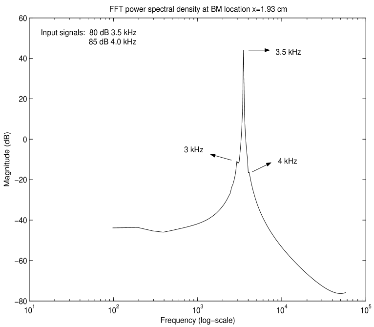
Figure 1: Time series of BM displacement at $x=1.93$ cm (top frame), and its FFT power spectral density vs. frequency (bottom frame).

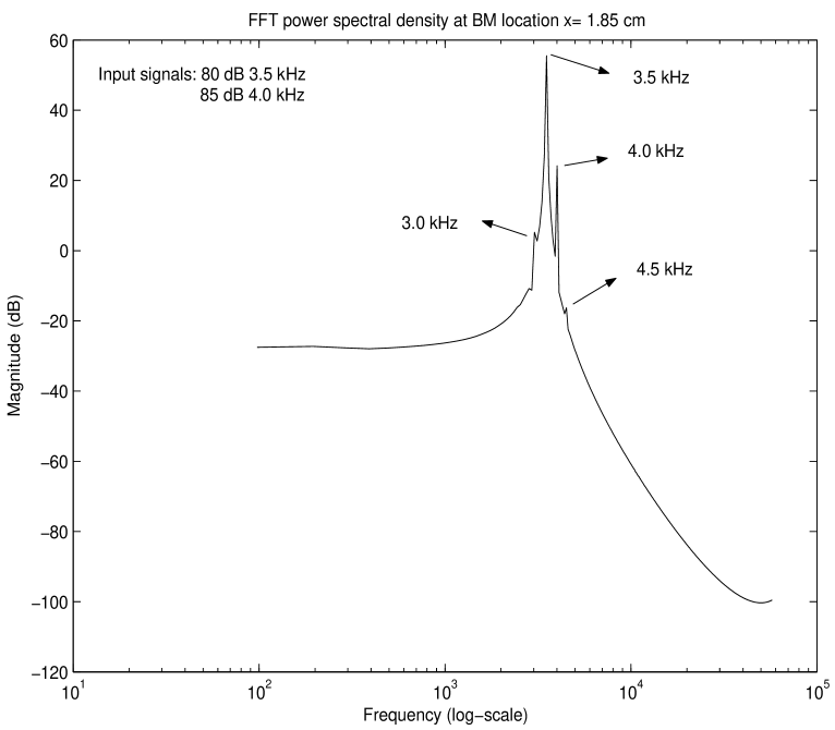
Figure 2: Time series of BM displacement at $x=1.85$ cm (top frame), and its FFT power spectral density vs. frequency (bottom frame).

Figure 3: Time series of BM displacement at $x=2.03$ cm (top frame), and its FFT power spectral density vs. frequency (bottom frame).

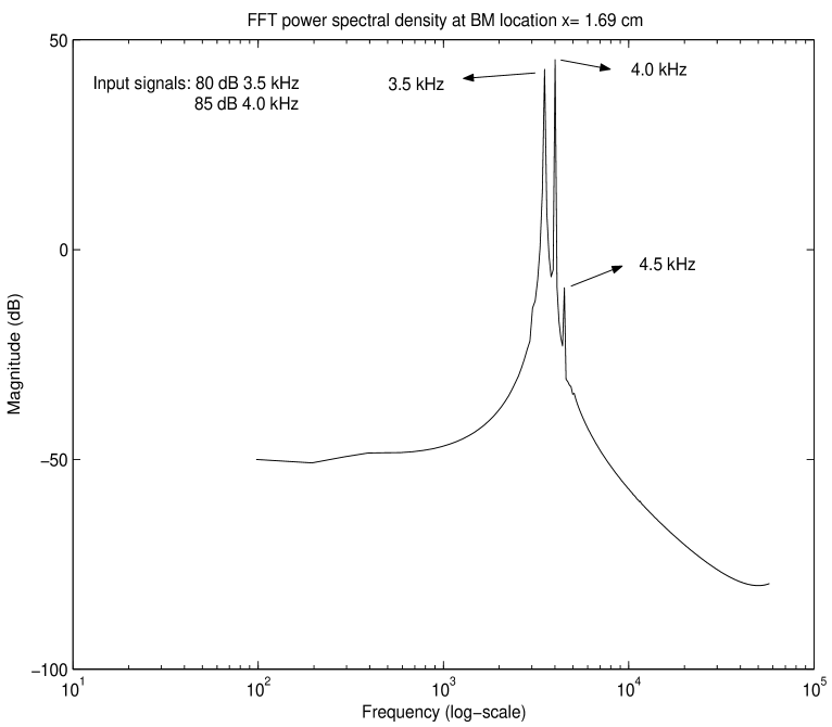
Figure 4: Time series of BM displacement at $x=1.69$ cm (top frame), and its FFT power spectral density vs. frequency (bottom frame).