Lagrangian dispersion in Gaussian
self-similar velocity ensembles
 

Abstract

We analyze the Lagrangian flow in a family of simple Gaussian scale-invariant velocity ensembles that exhibit both spatial roughness and temporal correlations. We show that the behavior of the Lagrangian dispersion of pairs of fluid particles in such models is determined by the scale dependence of the ratio between the correlation time of velocity differences and the eddy turnover time. For a non-trivial scale dependence, the asymptotic regimes of the dispersion at small and large scales are described by the models with either rapidly decorrelating or frozen velocities. In contrast to the decorrelated case, known as the Kraichnan model and exhibiting Lagrangian flows with deterministic or stochastic trajectories, fast separating or trapped together, the frozen model is poorly understood. We examine the pair dispersion behavior in its simplest, one-dimensional version, reinforcing analytic arguments by numerical analysis. The collected information about the pair dispersion statistics in the limiting models allows to partially predict the extent of different phases and the scaling properties of the Lagrangian flow in the model with time-correlated velocities.

1 Introduction

The aim of this paper is to study the Lagrangian flow in $d$-dimensional random velocity fields $\,{\mathchoice{{\hbox{\boldmath$\displaystyle v$}}}{{\hbox{\boldmath$\textstyle v$}}}{{\hbox{\boldmath$\scriptstyle v$}}}{{\hbox{\boldmath$\scriptscriptstyle v$}}}}(t,{\mathchoice{{\hbox{\boldmath$\displaystyle r$}}}{{\hbox{\boldmath$\textstyle r$}}}{{\hbox{\boldmath$\scriptstyle r$}}}{{\hbox{\boldmath$\scriptscriptstyle r$}}}})\,$ with a prescribed scale-invariant statistics. The velocity ensembles that we shall consider mimic some essential properties of realistic velocities in developed turbulence: their spatial roughness within a large interval of scales and their temporal correlation. By definition, the Lagrangian flow is described by the ordinary differential equation

$${d{\mathchoice{{\hbox{\boldmath$\displaystyle R$}}}{{\hbox{\boldmath$\textstyle R$}}}{{\hbox{\boldmath$\scriptstyle R$}}}{{\hbox{\boldmath$\scriptscriptstyle R$}}}}\over dt}\ =\ {\mathchoice{{\hbox{\boldmath$\displaystyle v$}}}{{\hbox{\boldmath$\textstyle v$}}}{{\hbox{\boldmath$\scriptstyle v$}}}{{\hbox{\boldmath$\scriptscriptstyle v$}}}}(t,{\mathchoice{{\hbox{\boldmath$\displaystyle R$}}}{{\hbox{\boldmath$\textstyle R$}}}{{\hbox{\boldmath$\scriptstyle R$}}}{{\hbox{\boldmath$\scriptscriptstyle R$}}}})\,.$$ (1.1)

It determines the motion of hypothetical fluid particles or of small test particles suspended in the fluid. One usually distinguishes between the motion of a single particle, dominated by the velocity fluctuations on the largest scale present (the so called ”sweeping effects”) and the evolution of a relative separation of two particles, the object of interest of the present paper, driven by the velocity fluctuations on scales of the order of the inter-particle distance. For larger groups of particles, one should similarly distinguish the motion of their barycenter from the relative motion of particles within the group. The latter is known to show quite intricate behavior related to intermittency, see [10], but it will not interest us here.

The separation $\,{\mathchoice{{\hbox{\boldmath$\displaystyle\rho$}}}{{\hbox{\boldmath$\textstyle\rho$}}}{{\hbox{\boldmath$\scriptstyle\rho$}}}{{\hbox{\boldmath$\scriptscriptstyle\rho$}}}}={\mathchoice{{\hbox{\boldmath$\displaystyle R$}}}{{\hbox{\boldmath$\textstyle R$}}}{{\hbox{\boldmath$\scriptstyle R$}}}{{\hbox{\boldmath$\scriptscriptstyle R$}}}}^{\prime}-{\mathchoice{{\hbox{\boldmath$\displaystyle R$}}}{{\hbox{\boldmath$\textstyle R$}}}{{\hbox{\boldmath$\scriptstyle R$}}}{{\hbox{\boldmath$\scriptscriptstyle R$}}}}\,$ between two fluid particles satisfies the equation

$${d{\mathchoice{{\hbox{\boldmath$\displaystyle\rho$}}}{{\hbox{\boldmath$\textstyle\rho$}}}{{\hbox{\boldmath$\scriptstyle\rho$}}}{{\hbox{\boldmath$\scriptscriptstyle\rho$}}}}\over dt}={\mathchoice{{\hbox{\boldmath$\displaystyle v$}}}{{\hbox{\boldmath$\textstyle v$}}}{{\hbox{\boldmath$\scriptstyle v$}}}{{\hbox{\boldmath$\scriptscriptstyle v$}}}}(t,{\mathchoice{{\hbox{\boldmath$\displaystyle\rho$}}}{{\hbox{\boldmath$\textstyle\rho$}}}{{\hbox{\boldmath$\scriptstyle\rho$}}}{{\hbox{\boldmath$\scriptscriptstyle\rho$}}}}+{\mathchoice{{\hbox{\boldmath$\displaystyle R$}}}{{\hbox{\boldmath$\textstyle R$}}}{{\hbox{\boldmath$\scriptstyle R$}}}{{\hbox{\boldmath$\scriptscriptstyle R$}}}}(t))-{\mathchoice{{\hbox{\boldmath$\displaystyle v$}}}{{\hbox{\boldmath$\textstyle v$}}}{{\hbox{\boldmath$\scriptstyle v$}}}{{\hbox{\boldmath$\scriptscriptstyle v$}}}}(t,{\mathchoice{{\hbox{\boldmath$\displaystyle R$}}}{{\hbox{\boldmath$\textstyle R$}}}{{\hbox{\boldmath$\scriptstyle R$}}}{{\hbox{\boldmath$\scriptscriptstyle R$}}}}(t))\,,$$ (1.2)

where ${\mathchoice{{\hbox{\boldmath$\displaystyle R$}}}{{\hbox{\boldmath$\textstyle R$}}}{{\hbox{\boldmath$\scriptstyle R$}}}{{\hbox{\boldmath$\scriptscriptstyle R$}}}}(t)$ is a trajectory of one of the particles, a solution of Eq.  (1.1) starting at time zero at ${\mathchoice{{\hbox{\boldmath$\displaystyle R$}}}{{\hbox{\boldmath$\textstyle R$}}}{{\hbox{\boldmath$\scriptstyle R$}}}{{\hbox{\boldmath$\scriptscriptstyle R$}}}}=0$,  for example. Upon introduction of the so called quasi-Lagrangian velocity,

$${\mathchoice{{\hbox{\boldmath$\displaystyle v$}}}{{\hbox{\boldmath$\textstyle v$}}}{{\hbox{\boldmath$\scriptstyle v$}}}{{\hbox{\boldmath$\scriptscriptstyle v$}}}}^{qL}(t,{\mathchoice{{\hbox{\boldmath$\displaystyle r$}}}{{\hbox{\boldmath$\textstyle r$}}}{{\hbox{\boldmath$\scriptstyle r$}}}{{\hbox{\boldmath$\scriptscriptstyle r$}}}})={\mathchoice{{\hbox{\boldmath$\displaystyle v$}}}{{\hbox{\boldmath$\textstyle v$}}}{{\hbox{\boldmath$\scriptstyle v$}}}{{\hbox{\boldmath$\scriptscriptstyle v$}}}}(t,{\mathchoice{{\hbox{\boldmath$\displaystyle r$}}}{{\hbox{\boldmath$\textstyle r$}}}{{\hbox{\boldmath$\scriptstyle r$}}}{{\hbox{\boldmath$\scriptscriptstyle r$}}}}+{\mathchoice{{\hbox{\boldmath$\displaystyle R$}}}{{\hbox{\boldmath$\textstyle R$}}}{{\hbox{\boldmath$\scriptstyle R$}}}{{\hbox{\boldmath$\scriptscriptstyle R$}}}}(t))\,,$$ (1.3)

i.e.  velocity in the frame moving with a fixed fluid particle, we may rewrite Eq.  (1.2) as

$${d{\mathchoice{{\hbox{\boldmath$\displaystyle\rho$}}}{{\hbox{\boldmath$\textstyle\rho$}}}{{\hbox{\boldmath$\scriptstyle\rho$}}}{{\hbox{\boldmath$\scriptscriptstyle\rho$}}}}\over dt}={\mathchoice{{\hbox{\boldmath$\displaystyle v$}}}{{\hbox{\boldmath$\textstyle v$}}}{{\hbox{\boldmath$\scriptstyle v$}}}{{\hbox{\boldmath$\scriptscriptstyle v$}}}}^{qL}(t,{\mathchoice{{\hbox{\boldmath$\displaystyle\rho$}}}{{\hbox{\boldmath$\textstyle\rho$}}}{{\hbox{\boldmath$\scriptstyle\rho$}}}{{\hbox{\boldmath$\scriptscriptstyle\rho$}}}})-{\mathchoice{{\hbox{\boldmath$\displaystyle v$}}}{{\hbox{\boldmath$\textstyle v$}}}{{\hbox{\boldmath$\scriptstyle v$}}}{{\hbox{\boldmath$\scriptscriptstyle v$}}}}^{qL}(t,\mathchoice{{\hbox{\boldmath$\displaystyle 0$}}}{{\hbox{\boldmath$\textstyle 0$}}}{{\hbox{\boldmath$\scriptstyle 0$}}}{{\hbox{\boldmath$\scriptscriptstyle 0$}}})\equiv\Delta{\mathchoice{{\hbox{\boldmath$\displaystyle v$}}}{{\hbox{\boldmath$\textstyle v$}}}{{\hbox{\boldmath$\scriptstyle v$}}}{{\hbox{\boldmath$\scriptscriptstyle v$}}}}^{qL}(t,{\mathchoice{{\hbox{\boldmath$\displaystyle\rho$}}}{{\hbox{\boldmath$\textstyle\rho$}}}{{\hbox{\boldmath$\scriptstyle\rho$}}}{{\hbox{\boldmath$\scriptscriptstyle\rho$}}}})\,.$$ (1.4)

We shall be interested in the short- and long-time behaviors of the Lagrangian particles in the statistical ensembles where typical velocities are only Hölder continuous in space. In such non-Lipschitz velocities, there is a problem with solving Eqs. (1.1), (1.2) or (1.4). To avoid it, we shall first consider noisy particle trajectories that solve the stochastic equation

$$d{\mathchoice{{\hbox{\boldmath$\displaystyle R$}}}{{\hbox{\boldmath$\textstyle R$}}}{{\hbox{\boldmath$\scriptstyle R$}}}{{\hbox{\boldmath$\scriptscriptstyle R$}}}}\ =\ {\mathchoice{{\hbox{\boldmath$\displaystyle v$}}}{{\hbox{\boldmath$\textstyle v$}}}{{\hbox{\boldmath$\scriptstyle v$}}}{{\hbox{\boldmath$\scriptscriptstyle v$}}}}(t,{\mathchoice{{\hbox{\boldmath$\displaystyle R$}}}{{\hbox{\boldmath$\textstyle R$}}}{{\hbox{\boldmath$\scriptstyle R$}}}{{\hbox{\boldmath$\scriptscriptstyle R$}}}})\,dt\,+\,\sqrt{2\kappa}\,d{\mathchoice{{\hbox{\boldmath$\displaystyle W$}}}{{\hbox{\boldmath$\textstyle W$}}}{{\hbox{\boldmath$\scriptstyle W$}}}{{\hbox{\boldmath$\scriptscriptstyle W$}}}}\,,$$ (1.5)

where $\,{\mathchoice{{\hbox{\boldmath$\displaystyle W$}}}{{\hbox{\boldmath$\textstyle W$}}}{{\hbox{\boldmath$\scriptstyle W$}}}{{\hbox{\boldmath$\scriptscriptstyle W$}}}}(t)\,$ is the Brownian motion in $\,d\,$ dimensions. Noisy trajectories form a well defined Markov process even in velocity fields with poor regularity. Subsequently, the limit $\kappa\to 0$ will be performed in selected quantities. The velocity ensembles that we shall consider are time-reversal invariant. As a result, we shall not have to distinguish the forward and the backward evolution of trajectories and will concentrate on the first one, between, say, times $0$ and $t$.

One way to study the relative motion of pairs of fluid particles is to follow the evolution of the pair dispersion, i.e.  of the separation distance $\,\rho\,$ between two particles. Its statistics in a random flow may be described by the velocity-averaged probability distribution $\,{\cal P}(\rho_{0},\rho;t)\,d\rho\,$ of the time $t$ dispersion $\,\rho\,$ given its time zero value $\,\rho_{0}$,  in the limit when we remove the (independent) noises of the Lagrangian trajectories. As we shall see, the PDF’s $\,{\cal P}(\rho_{0},\rho;t)\,$ may be sometimes distributions rather than integrable functions. Another, related, test of the relative motion of a pair of fluid particles is obtained by looking at the exit time [17, 4]: the time $\,t\,$ that the pair dispersion takes to evolve from $\,\rho_{0}$ to $\,\rho_{1}$. In particular, $\,\rho_{1}=2\rho_{0}\,$ corresponds to the doubling time of the pair dispersion. The statistics of the exit times may be encoded in their velocity-averaged probability distribution $\,{\cal Q}(t;\rho_{0},\rho_{1})\,dt\,$ taken in the limit of vanishing noise. The exit time is less influenced than the pair dispersion by small or large-distance cutoffs in the velocity correlations, so preferable in numerical or experimental studies [4].

Recently, a new insight into the intricate character of the Lagrangian flow in turbulent velocities has been gained, see [3, 19, 24, 30, 25], by analytic study of the Kraichnan ensemble [23] of Gaussian velocities which are decorrelated in time but exhibit scaling behavior in space. Here, we try to find out how the presence of temporal correlations of velocities influences the Lagrangian flow. We shall study the behavior of trajectory separation in a simple generalization of the Kraichnan ensemble of velocities where time correlations are reintroduced.

The paper is organized as follows. In Sect. 2 we recall the main facts about the Lagrangian flow in the Kraichnan model, in particular the appearance of phases with very different trajectory behavior. Sect. 3 describes a Gaussian ensemble of velocities with temporal correlations, discussed in the past in [8, 2, 11, 14]. It exposes a simple mean-field type analysis of the particle separation when such an ensemble is used to model the quasi-Lagrangian velocities. How the mean-field predictions may be substantiated further by scaling arguments is the subject of Sect. 4. See also [12, 13] for related rigorous results. Analytic arguments and conjectures about the behavior of trajectories in a one-dimensional version of the model with time-independent velocities are contained in Sect. 5. The behavior of the exit time statistics in velocity ensembles with long-time correlations is studied in Sect.  6. The question how the behavior of pair dispersion changes when the Gaussian ensemble is used to model the Eulerian velocities is addressed in Sect. 7. In particular we show that in the one-dimensional time-independent case, the sweeping by large eddies in the Eulerian model speeds up the movement of a single Lagrangian particle but it localizes pairs of particles by reducing the growth of their dispersion. Three Appendices contain more technical material. Some of the predictions of the paper are checked in one dimension by numerical simulations.

Acknowledgements: The work of MC was supported by the Fundação para a Ciência e a Tecnologia grant: PRAXIS XXI/BD/21413/99. KG, PH, AK and MV are grateful to the Erwin Schrödinger Institute in Vienna and the Institute for Advanced Study in Princeton where parts of the work on the paper were done. KG acknowledges the support of the Neumann Fund and MV the Ralph E. and Doris M. Hansmann Membership at the IAS. AK and MV were also supported by the European Union under the Contracts FMRX-CT98-0175 and HPRN-CT-2000-00162, respectively.

2 Lessons from the Kraichnan model

The Kraichnan ensemble of turbulent velocities [23], is a Gaussian ensemble with vanishing velocity 1-point function and with the 2-point function

$$\Big{\langle}v^{i}(t,{\mathchoice{{\hbox{\boldmath$\displaystyle r$}}}{{\hbox{\boldmath$\textstyle r$}}}{{\hbox{\boldmath$\scriptstyle r$}}}{{\hbox{\boldmath$\scriptscriptstyle r$}}}})\,v^{j}(t^{\prime},{\mathchoice{{\hbox{\boldmath$\displaystyle r$}}}{{\hbox{\boldmath$\textstyle r$}}}{{\hbox{\boldmath$\scriptstyle r$}}}{{\hbox{\boldmath$\scriptscriptstyle r$}}}}^{\prime})\Big{\rangle}\ =\ D_{1}\,\,\delta(t-t^{\prime})\int{{\rm e}^{\,\,i\,{\mathchoice{{\hbox{\boldmath$\displaystyle k$}}}{{\hbox{\boldmath$\textstyle k$}}}{{\hbox{\boldmath$\scriptstyle k$}}}{{\hbox{\boldmath$\scriptscriptstyle k$}}}\cdot({\mathchoice{{\hbox{\boldmath$\displaystyle r$}}}{{\hbox{\boldmath$\textstyle r$}}}{{\hbox{\boldmath$\scriptstyle r$}}}{{\hbox{\boldmath$\scriptscriptstyle r$}}}}-{\mathchoice{{\hbox{\boldmath$\displaystyle r$}}}{{\hbox{\boldmath$\textstyle r$}}}{{\hbox{\boldmath$\scriptstyle r$}}}{{\hbox{\boldmath$\scriptscriptstyle r$}}}}^{\prime})}}\over{k_{{}_{L}}^{d+\xi}}}\,\,P^{ij}({\mathchoice{{\hbox{\boldmath$\displaystyle k$}}}{{\hbox{\boldmath$\textstyle k$}}}{{\hbox{\boldmath$\scriptstyle k$}}}{{\hbox{\boldmath$\scriptscriptstyle k$}}}},\wp)\,\,{{d{\mathchoice{{\hbox{\boldmath$\displaystyle k$}}}{{\hbox{\boldmath$\textstyle k$}}}{{\hbox{\boldmath$\scriptstyle k$}}}{{\hbox{\boldmath$\scriptscriptstyle k$}}}}}\over{(2\pi)^{d}}}\,,$$ (2.1)

where $\,k_{{}_{L}}=\sqrt{k^{2}+L^{-2}}\,$ and $\,P^{ij}({\mathchoice{{\hbox{\boldmath$\displaystyle k$}}}{{\hbox{\boldmath$\textstyle k$}}}{{\hbox{\boldmath$\scriptstyle k$}}}{{\hbox{\boldmath$\scriptscriptstyle k$}}}},\wp)={1-\wp\over d-1}\Big{(}\delta^{ij}-{k^{i}k^{j}\over k^{2}}\Big{)}+\wp{k^{i}k^{j}\over k^{2}}$, see [10] and references therein. There are two dimensionless parameters in the Kraichnan ensemble: the exponent $\,\xi>0\,$ and the compressibility degree $\,0\leq\wp\leq 1$. For $\,\xi\leq 2$, the velocities smeared in time are (almost surely) Hölder continuous in space with any exponent smaller than $\xi/2$. For $\,\xi>2$, they are Lipschitz (or even more regular). The compressibility degree $\,\wp=0\,$ corresponds to incompressible velocities, $\,\wp=1\,$ to gradients of a potential (in one dimension necessarily $\wp=1$).  The normalization constant $\,D_{1}\,$ has dimension $\,length^{2-\xi}/time$.  The length $L$ is the integral scale that sets the spatial correlation length of velocities. If $\,\xi<2$,  it may be taken to infinity in the correlation functions involving only velocity differences $\,{\mathchoice{{\hbox{\boldmath$\displaystyle v$}}}{{\hbox{\boldmath$\textstyle v$}}}{{\hbox{\boldmath$\scriptstyle v$}}}{{\hbox{\boldmath$\scriptscriptstyle v$}}}}(t,{\mathchoice{{\hbox{\boldmath$\displaystyle r$}}}{{\hbox{\boldmath$\textstyle r$}}}{{\hbox{\boldmath$\scriptstyle r$}}}{{\hbox{\boldmath$\scriptscriptstyle r$}}}}+{\mathchoice{{\hbox{\boldmath$\displaystyle\rho$}}}{{\hbox{\boldmath$\textstyle\rho$}}}{{\hbox{\boldmath$\scriptstyle\rho$}}}{{\hbox{\boldmath$\scriptscriptstyle\rho$}}}})-{\mathchoice{{\hbox{\boldmath$\displaystyle v$}}}{{\hbox{\boldmath$\textstyle v$}}}{{\hbox{\boldmath$\scriptstyle v$}}}{{\hbox{\boldmath$\scriptscriptstyle v$}}}}(t,{\mathchoice{{\hbox{\boldmath$\displaystyle r$}}}{{\hbox{\boldmath$\textstyle r$}}}{{\hbox{\boldmath$\scriptstyle r$}}}{{\hbox{\boldmath$\scriptscriptstyle r$}}}})\equiv\Delta{\mathchoice{{\hbox{\boldmath$\displaystyle v$}}}{{\hbox{\boldmath$\textstyle v$}}}{{\hbox{\boldmath$\scriptstyle v$}}}{{\hbox{\boldmath$\scriptscriptstyle v$}}}}(t,{\mathchoice{{\hbox{\boldmath$\displaystyle\rho$}}}{{\hbox{\boldmath$\textstyle\rho$}}}{{\hbox{\boldmath$\scriptstyle\rho$}}}{{\hbox{\boldmath$\scriptscriptstyle\rho$}}}})$.  For $\,\xi\geq 2$, this may still be done if $\,D_{1}\,$ is rescaled when $\,L\to\infty$.

A  Possible flow behaviors

The Kraichnan ensemble may be used invariably to model Eulerian or quasi-Lagrangian velocities as both ensembles coincide in this case. The statistics of a single Lagrangian particle is that of a $d$-dimensional Brownian motion with diffusivity that blows up when $\,L\to 0$.  The two-particle separation depends only on velocity differences and its statistics has a non-trivial $\,L\to\infty\,$ limit whenever this holds for the velocity differences. The pair-dispersion and the exit time PDF’s $\,{\cal P}(\rho_{0},\rho;t)\,$ and $\,{\cal Q}(t;\rho_{0},\rho_{1})\,$ may be solved analytically in this limit. The exact solutions, that describes also the short-distance asymptotics of the PDF’s at finite $\,L$,  show several dichotomic behaviors depending on the values of parameters of the model. The first dichotomy, noticed in [3], is between the

deterministic flow characterized by the property

$$\lim\limits_{\rho_{0}\to 0}\,\,{\cal P}(\rho_{0},\rho;t)\ =\ \delta(\rho)$$ (2.2)

which signals that the trajectories in a fixed velocity field are defined by their initial position, and the

stochastic flow where

$$\lim\limits_{\rho_{0}\to 0}\,\,{\cal P}(\rho_{0},\rho;t)\quad{\rm is\ an\ integrable\ function\ of\ }\ \,\rho\,.$$ (2.3)

The limits of the PDF’s above (and below) should be understood in weak sense, under integrals against test functions. The behavior (2.3) means that infinitesimally close trajectories separate in a finite time and indicates that the stochasticity introduced into the Lagrangian flow by coupling it to the noise, see Eq.  (1.5), survives in the limit $\kappa\to\nobreak 0$.  The Lagrangian trajectories in a fixed velocity field are not determined by initial position but form instead a stochastic process. That this is indeed what happens in the Kraichnan model was established rigorously in [24]. We shall call the phenomenon spontaneous stochasticity.

There are further dichotomic behaviors of the Lagrangian flow in the Kraichnan model. We have chosen to characterize the other dichotomies in terms of the small $\,\rho_{0}\,$ behavior of the exit time PDF $\,{\cal Q}(t;\rho_{0},\gamma\rho_{0})\,$ with $\,0<\gamma={\rm const}.\not=1$,  attaching to them more or less suggestive names.  There is a dichotomy between the

Lyapunov flow such that

$$\lim\limits_{\rho_{0}\to 0}\,\,{\cal Q}(t;\rho_{0},\gamma\rho_{0})\quad{\rm is\ an\ integrable\ function\ of}\ \,t\,,$$ (2.4)

and the

Richardson flow where

$$\lim\limits_{\rho_{0}\to 0}\,\,{\cal Q}(t;\rho_{0},\gamma\rho_{0})\ =\ c(\gamma)\,\delta(t)\quad{\rm with\ }\ c(\gamma)>0\,.$$ (2.5)

This dichotomy distinguishes the flows in regular velocities where the Lagrangian separation on short distances involves fixed time scales (like the inverse Lyapunov exponent), from the ones in non-regular (non-Lipschitz) velocities where the characteristic times of the Lagrangian separation become very short on short scales.

Finally, the last two dichotomies that we want to single out characterize the short distance behavior of the probability of infinite exit times. They are between the

locally separating  and  locally trapping flow where for $\,\gamma>1$

$$\lim\limits_{\rho_{0}\to 0}\int{\cal Q}(t;\rho_{0},\gamma\rho_{0})\,dt\ \cases{\ =\ \cr\ <\ }\Big{\}}\ 1\,,\ \,{\rm respectively},$$ (2.6)

and

locally recurrent  and  locally transient flow where the same holds for $\,\gamma<1$.

Roughly, with positive probability, close trajectories do not increase their distance in locally trapping flows and do not approach each other in locally transient ones.

B  Pair dispersion

Due to the temporal decorrelation of the Kraichnan velocities, the probability measures $\,{\cal P}(\rho_{0},\rho;t)\,d\rho\,$ constitute transition probabilities of a Markov process $\,\rho(t)\,$ that in the limit $\,L\to\infty\,$ becomes a diffusion on a half-line with the explicit generator

$$M\ =\ -D_{1}^{\prime}\,\rho^{\xi-a}\partial_{\rho}\,\rho^{a}\partial_{\rho}\qquad{\rm for}\ \quad a\,=\,{{}_{d+\xi}\over{}^{1+\wp\xi}}-1\,,$$ (2.7)

where $\,D_{1}^{\prime}$ is proportional to $D_{1}$.  Note that the symbol of $\,M\,$ vanishes at $\,\rho=0$.  The different behavior of such diffusion for different values of $\,\xi\,$ and $\,a\,$ has its origin in the singularity of $\,M\,$ at $\,\rho=0\,$ which requires different treatment in different regimes. Up to the change of variables $\,x=\rho^{(2-\xi)/2}\,$ casting the generator $\,M\,$ into the form

$$M\ =\ {{}_{1}\over{}^{4}}(2-\xi)^{2}D^{\prime}\,x^{1-\delta}\partial_{x}x^{\delta-1}\partial_{x}\qquad{\rm for}\ \quad\delta\,=\,2(1-{{}_{1-a}\over{}^{2-\xi}})$$ (2.8)

and a time rescaling, the Markov process $\,\rho(t)\,$ may be identified with the well studied Bessel diffusion [5], a natural interpolation between processes describing the radial variable in the standard diffusion in dimensions $\,\delta$. Various analytic formulae may be then directly carried from that case to the present situation.

For $\,\xi=2\,$ corresponding to smooth velocities with velocity differences linear in space, the particle dispersion PDF takes a log-normal form [7, 9]:

$${\cal P}(\rho_{0},\rho;t)\ \ \ \propto\ \ {\rm e}^{-{1\over 4D_{1}^{\prime}t}\,(\ln(\rho/\rho_{0})\,-\,\lambda t)^{2}}\,\rho^{-1}\,,$$ (2.9)

where $\,\lambda={d-4\wp\over 1+2\wp}D_{1}^{\prime}\,$ is the (biggest) Lyapunov exponent.  It is easy to see that in this case, $\,\lim\limits_{\rho_{0}\to 0}\,{\cal P}(\rho_{0},\rho;t)=\delta(\rho)$,  pointing to the deterministic nature of the flow. Indeed, in velocities regular in space the trajectories are uniquely determined by their initial position and very close fluid particles separate little in a fixed time interval. Nevertheless, all moments of the pair dispersion behave exponentially in time and grow in the chaotic regime where $\,\lambda>0$,  i.e. $\wp<{d/4}$,  whereas sufficiently small (fractional) ones decrease when $\,\lambda<0$, i.e. $\wp>{d/4}$. For the second moment, one obtains:

$$\langle\,\rho^{2}(t)\,\rangle\ =\ {\rm e}^{\,(2\lambda+4D_{1}^{\prime})\,t}\,\rho_{0}^{2}\,.$$ (2.10)

Similar behaviors persist at small times in the Kraichnan velocities with $\,\xi>2\,$ and finite $\,L$, see [24].

The stochastic Lagrangian flow occurs in the non-Lipschitz version with $\,0<\xi<2\,$ of the Kraichnan model for weak compressibility $\,\wp<d/\xi^{2}$.  In terms of the parameter $\,b={1-a\over 2-\xi}={2-\delta\over 2}\,$ that will be frequently used below, the latter inequality means that $\,b<1$.  In this region, $\,{\cal P}(\rho_{0},\rho;t)={\rm e}^{-t\,M}(\rho_{0},\rho)\,$ where $\,M\,$ is taken with “singular Neumann” or reflecting boundary condition at $\,\rho=0$, see [19], and

$$\lim\limits_{\rho_{0}\to 0}\ {\cal P}(0,\rho;t)\ \ \propto\ \ \rho^{a-\xi}\,t^{b-1}\,\,{\rm e}^{-{\rho^{2-\xi}\over(2-\xi)^{2}D_{1}^{\prime}\,t}}\,.$$ (2.11)

Note the stretched-exponential form of the PDF. In particular, one obtains for the second moment of the separation distance and large times:

$$\langle\,\rho^{2}(t)\,\rangle\ =\ {\cal O}(t^{2\over 2-\xi})\,.$$ (2.12)

This is the Kraichnan model version of the 1926 Richardson law [28] stating that in developed turbulence the mean square dispersion grows like $\,t^{3}$.  Note that the Richardson behavior is reproduced in the Kraichnan model for $\,\xi={4\over 3}$. In the limit when the initial trajectory separation $\,\rho_{0}\to 0$,   the power law behavior (2.12) extends to the entire time domain and $\,\langle\rho^{2}(t)\rangle\propto\,t^{2\over 2-\xi}$.

In the non-Lipschitz strongly compressible version of the Kraichnan model corresponding to $\,0<\xi<2\,$ and $\,\wp\geq d/\xi^{2}\,$ (or $\,b\geq 1$),

$${\cal P}(\rho_{0},\rho;t)\ =\ {\cal P}^{\rm reg}(\rho_{0},\rho;t)\ +\ p(\rho_{0};t)\,\delta(\rho)$$ (2.13)

with the regular part of the PDF $\,{\cal P}^{\rm reg}(\rho_{0},\rho;t)={\rm e}^{-t\,M}(\rho_{0},\rho)\,$ where $\,M\,$ is taken with “singular Dirichlet” or absorbing boundary condition at $\,\rho=0$,  see [19], and with

$$p(\rho_{0};t)\ =\ 1-\gamma\left(b,{{}_{\rho_{0}^{2-\xi}}\over{}^{(2-\xi)^{2}D_{1}^{\prime}\,t}}\right)\,\Gamma(b)^{-1}\,,$$ (2.14)

where $\ \gamma(b,x)\equiv\int\limits_{0}^{x}y^{b-1}\,{\rm e}^{-y}\,dy\$ is the incomplete gamma-function. When $\,\rho_{0}\to 0\,$ then the regular part of the PDF tends to $\,0$,  whereas $\,p(\rho_{0};t)\,$ tends to $\,1$.  We recover this way the deterministic behavior (2.2), with trajectories in fixed velocity realizations determined by their initial position.  The presence of the term proportional to $\,\delta(\rho)\,$ at finite $\,\rho_{0}\,$ signals that the trajectories starting at different initial positions coalesce with positive probability [19]. The time growth of the mean distance square dispersion is different here:

$$\langle\,\rho^{2}(t)\,\rangle\ =\ {\cal O}(\rho_{0}^{1-a}\,t^{{2\over 2-\xi}-b})$$ (2.15)

with a logarithmic correction at $\,\wp=d/\xi^{2}\,$ i.e.  at $\,b=1$.

C  Exit time

In the Kraichnan model, the exit time PDF $\,{\cal Q}(t;\rho_{0},\rho_{1})\,$ may also be directly controlled using the kernels $\,{\rm e}^{-t\,M_{D}}(\rho_{0},\rho)\,$ where $\,M_{D}\,$ denotes the generator $\,M\,$ of (2.7) with the Dirichlet boundary condition at $\,\rho_{1}\,$ (in addition to the appropriate condition at the origin when $\,\rho_{1}>\rho_{0}$). This is due to the Markov property of the stochastic process $\,\rho(t)$.  Since the exit times have not been discussed in the context of the Kraichanan model, we shall use the occasion to provide more details, essentially translated form the Bessel diffusion case.  The PDF of the time of exit through $\,\rho_{1}\,$ is given by

$${\cal Q}(t;\rho_{0},\rho_{1})\ =\ -\partial_{n(\rho_{1})}\,{\rm e}^{-t\,M_{D}}(\rho_{0},\rho)\,,$$ (2.16)

where $\,\partial_{n(\rho_{1})}=\pm\,D_{1}^{\prime}\,\rho^{a}\partial_{\rho}\,\rho^{\xi-a}|_{\rho=\rho_{1}}\,$ plays here the same role as the normal derivative in the classical potential theory. The sign is that of $\,(\rho_{1}-\rho_{0})$.  This PDF does not have to integrate to $\,1$.  The eventual missing probability corresponds to events where $\,\rho(t)\,$ stays forever in the open interval $\,(0,\rho_{1})\,$ or $\,(\rho_{1},\infty)\,$ or when it gets absorbed at the origin, see below. We shall assign the infinite value of the exit time to such events. The averages of the powers of the exit time $\,t\,$ over the realizations with $\,t<\infty\,$ may be expressed by the kernels of the inverse powers of operator $\,M_{D}$:

$$\langle\,t^{n}\,1_{\{t<\infty\}}\,\rangle\ =\int\limits_{0}^{\infty}t^{n}\,{\cal Q}(t;\rho_{0},\rho_{1})\,dt\ =\ -\,n!\,\partial_{n(\rho_{1})}M_{D}^{-n-1}(\rho_{0},\rho;t)\,,$$ (2.17)

where by $\,1_{\{A\}}\,$ we denote the characteristic functions of the events satisfying the condition $\,A$.  In particular, the probability that the exit time is finite

$$\langle\,1_{\{t<\infty\}}\,\rangle\ =\int\limits_{0}^{\infty}\,{\cal Q}(t;\rho_{0},\rho_{1})\,dt\ =\ -\partial_{n(\rho_{1})}M_{D}^{-1}(\rho_{0},\rho;t)\,.$$ (2.18)

The expectations (2.17) may be obtained from the characteristic function

$$\langle\,{\rm e}^{i\omega t}\,1_{\{t<\infty\}}\,\rangle\ =\ -\partial_{n(\rho_{1})}(M_{D}-i\omega)^{-1}(\rho_{0},\rho_{1};t)$$ (2.19)

involving the resolvent kernel of $\,M_{D}$. We may also consider the averages conditioned on the exit times being finite:

$${\langle\,t^{n}\,1_{\{t<\infty\}}\,\rangle\over\langle\,1_{\{t<\infty\}}\,\rangle}\ \equiv\ \langle\,t^{n}\,\rangle_{{}_{c}}\,,\qquad{\langle\,{\rm e}^{i\omega t}\,1_{\{t<\infty\}}\,\rangle\over\langle\,1_{\{t<\infty\}}\,\rangle}\ \equiv\ \langle\,{\rm e}^{i\omega t}\,\rangle_{{}_{c}}\,.$$ (2.20)

For $\,\xi=2\,$ and $\,L=\infty$,  i.e.  in the smooth version of the Kraichnan model, the kernel $\,{\rm e}^{-t\,M_{D}}(\rho_{0},\rho)\,$ is easily calculable by the image method:

$${\rm e}^{-t\,M_{D}}(\rho_{0},\rho)\ =\ \,{{}_{1}\over{}^{\sqrt{4\pi D_{1}^{\prime}t}\,\rho}}\Big{(}{\rm e}^{-{1\over 4D_{1}^{\prime}t}\,(\ln(\rho/\rho_{0})\,-\,\lambda t)^{2}}-\,{\rm e}^{{\lambda\over D_{1}^{\prime}}\ln(\rho_{1}/\rho_{0})\,-\,{1\over 4D_{1}^{\prime}t}\,(\ln(\rho\rho_{0}/\rho_{1}^{2})-\lambda t)^{2}}\Big{)}\,.$$ (2.21)

For the exit time PDF, one obtains:

$${\cal Q}(t;\rho_{0},\rho_{1})\, = \,{{}_{|\ln(\rho_{1}/\rho_{0})|}\over{}^{\sqrt{4\pi D_{1}^{\prime}\,t^{3}}}}\,{\rm e}^{-{1\over{4D_{1}^{\prime}t}}(\ln(\rho_{1}/\rho_{0})-\lambda t)^{2}}$$ (2.22)

$$= \,{{}_{|\ln(\rho_{1}/\rho_{0})|}\over{}^{\sqrt{4\pi D_{1}^{\prime}\,t^{3}}}}\,{\rm e}^{{\lambda\,\ln(\rho_{1}/\rho_{0})\over{2D_{1}^{\prime}}}}\,{\rm e}^{-{1\over{4D_{1}^{\prime}t}}\ln^{2}(\rho_{1}/\rho_{0})\,-\,{\lambda^{2}\over{4D_{1}^{\prime}}}t}\,.$$ (2.23)

Note that the PDF depends only on $\,{\rho_{1}\over\rho_{0}}\,$ so that the corresponding Lagrangian flow is Lyapunov in our terminology, see (2.4). The total mass is given by the simple expression:

$$\int\limits_{0}^{\infty}{\cal Q}(t;\rho_{0},\rho_{1})\,dt\ =\ \cases{\ \hbox to76.82234pt{$1$\hfill}{\rm if}\qquad\lambda\,\ln(\rho_{1}/\rho_{0})\,\geq\,0\,,\cr\ \hbox to76.82234pt{$\left({{\rho_{1}}\over{\rho_{0}}}\right)^{{\lambda\over D_{1}^{\prime}}}$\hfill}{\rm if}\qquad\lambda\,\ln(\rho_{1}/\rho_{0})\,\leq\,0\,.}$$ (2.24)

The missing probability corresponds for $\,\rho_{1}>\rho_{0}\,$ and the negative Lyapunov exponent to the events when $\,\rho(t)\,$ stays forever in the open interval $\,(0,\rho_{1})\,$ (the pairs of trajectories remain always close). For $\,\rho_{1}<\rho_{0}\,$ and the positive Lyapunov exponent, it represents the events when $\,\rho(t)\,$ stays forever in the interval $\,(\rho_{1},\infty)\,$ (the pairs of trajectories never come close). According to the characterization from the previous subsection, see conditions (2.6), the Lagrangian flow is locally separating and locally transient if $\,\lambda>0$, i.e. $\wp<{d/4}$  and it is locally trapping and locally recurrent if $\,\lambda<0$, i.e. $\wp>{d/4}$.  Finally, when $\,\lambda=0$,  i.e. $\wp=d/4$,  it is locally separating and locally recurrent.  Similar properties of the exit time PDF hold for $\,\xi>2\,$ and finite $\,L\,$ asymptotically at short distances.

The exit time PDF (2.23) vanishes with all derivatives at $\,t=0\,$ and it has an exponentially decaying tail at large $\,t$. For the exit time conditional moments, one obtains:

$$\langle\,t^{n}\,\rangle_{{}_{c}}\, = \,{{}_{|\lambda|}\over{}^{\sqrt{\pi D_{1}^{\prime}}}}\,\left({{}_{|\ln(\rho_{1}/\rho_{0})|}\over{}^{|\lambda|}}\right)^{n+{{}_{1}\over{}^{2}}}{\rm e}^{{|\lambda\,\ln(\rho_{1}/\rho_{0})|\over 2D_{1}^{\prime}}}\,K_{|n+{{}_{1}\over{}^{2}}|}\left({{}_{|\lambda\,\ln(\rho_{1}/\rho_{0})|}\over{}^{2D_{1}^{\prime}}}\right)$$ (2.25)

$$= \,\sum\limits_{k=0}^{|n-{{}_{1}\over{}^{2}}|-{{}_{1}\over{}^{2}}}{{}_{(|n-{{}_{1}\over{}^{2}}|-{{}_{1}\over{}^{2}}+k)!}\over{}^{k!\,(|n-{{}_{1}\over{}^{2}}|-{{}_{1}\over{}^{2}}-k)!}}\,\left({{}_{D_{1}^{\prime}}\over{}^{\lambda^{2}}}\right)^{k}\,\left({{}_{|\ln(\rho_{1}/\rho_{0})|}\over{}^{|\lambda|}}\right)^{n-k},$$ (2.26)

where the first expression with the Bessel function holds for all real $n$ and the second one for integer $\,n$.  The unconditioned moments diverge for $\,n>0\,$ if $\,\lambda\,\ln(\rho_{1}/\rho_{0})<0\,$ due to the finite probability of infinite exit times. For the conditional characteristic function one obtains:

$$\langle\,{\rm e}^{i\omega t}\,\rangle_{{}_{c}}\ =\ \left({{}_{\rho_{1}}\over{}^{\rho_{0}}}\right)^{\pm{\lambda\over D_{1}^{\prime}}\Big{(}{1\over 2}\,-\,\sqrt{{1\over 4}-i{D_{1}^{\prime}\omega\over\lambda^{2}}}\Big{)}},$$ (2.27)

where the square root is taken with the positive real part and the sign is that of $\,\lambda\,\ln(\rho_{1}/\rho_{0})$.  The decay at large $\,|\omega|\,$ and the analyticity properties of the characteristic function reflect the behavior of the exit time PDF at small and large $\,t$.  In particular, the decay $\,\sim{\rm e}^{-|\ln(\rho_{1}/\rho_{0})|\sqrt{|\omega|/D^{\prime}_{1}}}\,$ of the characteristic function along the positive imaginary axis of $\,\omega\,$ signals the behavior $\,\sim{\rm e}^{-{1\over 4D^{\prime}_{1}\,t}\ln^{2}(\rho_{1}/\rho_{0})}\,$ of $\,{\cal Q}(t;\rho_{0},\rho_{1})\,$ for small $\,t\,$ and the singularity at $\,\omega=-i{\lambda^{2}\over 4D^{\prime}_{1}}\,$ indicates the presence of the tail $\,\sim{\rm e}^{-{\lambda^{2}\over 4D^{\prime}_{1}}t}\,$ for large $\,t$,  in agreement with Eq.  (2.23). Note non-Gaussian character of the large fluctuations of $\,t\,$ and of $\,t^{-1}$.

In the non-Lipschitz version of the Kraichnan model with $\,0<\xi<2$,  the resolvent kernel $\,(M_{D}-i\omega)^{-1}(\rho_{0},\rho)\,$ may still be easily calculated in a closed form. Let us start from the case with $\,\rho_{1}>\rho_{0}$. On the interval $\,[0,\rho_{1}]$,

$$(M_{D}-i\omega)^{-1}(\rho_{0},\rho)\ =\ {{}_{1}\over{}^{D_{1}^{\prime}}}\,{\cal W}^{-1}\,\rho^{a-\xi}\,f_{\mp}(\rho_{1})^{-1}$$ (2.28)

$$\hskip 56.9055pt\cdot\ \cases{\hbox to207.7052pt{$\,f_{\mp}(\rho_{0})\,(f_{\pm}(\rho)\,f_{\mp}(\rho_{1})\,-\,f_{\mp}(\rho)\,f_{\pm}(\rho_{1}))$\hfill}{\rm for}\quad\rho_{0}\leq\rho\,,\cr\hbox to207.7052pt{$\,f_{\mp}(\rho)\,(f_{\pm}(\rho_{0})\,f_{\mp}(\rho_{1})\,-\,f_{\mp}(\rho_{0})\,f_{\pm}(\rho_{1}))$\hfill}{\rm for}\quad\rho_{0}\geq\rho\,,}$$ (2.29)

where the upper sign pertains to the weakly compressible $\,\wp<{d\over\xi^{2}}\,$ region and the lower one to the strongly compressible one $\,\wp\geq{d\over\xi^{2}}$,  with $\,f_{\pm}\,$ giving two independent solutions of the eigenfunction equation $\,(M-i\omega)f=0\,$ expressed by the Bessel functions:

$$f_{\pm}(\rho)\ =\ \rho^{1-a\over 2}\,J_{\pm b}\left({{}_{2}\over{}^{2-\xi}}\sqrt{{{}_{i\omega}\over{}^{D_{1}^{\prime}}}\,\rho^{2-\xi}}\right)$$ (2.30)

and with

$${\cal W}\ =\ \rho^{a}\left(f_{\pm}(\rho)\partial_{\rho}f_{\mp}(\rho)\,-\,f_{\mp}(\rho)\partial_{\rho}f_{\pm}(\rho)\right)$$ (2.31)

standing for their $\rho$-independent Wronskian. The eigenfunction $\,f_{+}\,$ ($\,f_{-}$)  satisfies the singular Dirichlet (Neumann) condition at the origin imposed by the limit when the trajectory noise is turned off for weak (strong) compressibility, see [19]. It follows that

$$\langle\,{\rm e}^{i\omega t}\,1_{\{t<\infty\}}\,\rangle\ =\ -\partial_{n(\rho_{1})}(M-i\omega)^{-1}(\rho_{0},\rho_{1})\ =\ {{f_{\mp}(\rho_{0})}\over{f_{\mp}(\rho_{1})}}\,.$$ (2.32)

For $\,\omega\to 0\,$ the eigenfunction $\,f_{-}$ reduces to a constant whereas $\,f_{+}$ becomes proportional to $\,\rho^{1-a}$ so that

$$\langle\,1_{\{t<\infty\}}\,\rangle\ =\ \cases{\,\hbox to56.9055pt{$1$\hfill}{\rm for}\quad\wp<{d\over\xi^{2}}\,,\cr\,\hbox to56.9055pt{$\left({\rho_{0}\over\rho_{1}}\right)^{{}^{1-a}}$\hfill}{\rm for}\quad\wp\geq{d\over\xi^{2}}\,.}$$ (2.33)

Hence the exit time is almost surely finite in the weakly compressible regime whereas it is infinite with positive probability that depends only on $\,{\rho_{1}\over\rho_{0}}\,$ in the strongly compressible regime where the process $\,\rho(t)\,$ is absorbed at the origin with the complementary probability. Such absorption corresponds to the coalescence of pairs of trajectories. We conclude that the Lagrangian flow is locally separating for $\,\wp\leq d/\xi^{2}\,$ and locally trapping for $\,\wp>d/\xi^{2}$.

For the conditional characteristic function, one obtains

$$\langle\,{\rm e}^{i\omega t}\,\rangle_{{}_{c}}\ =\ \left({\rho_{0}\over\rho_{1}}\right)^{\mp{a-1\over 2}}\,{{J_{\mp b}\left({2\over{2-\xi}}\sqrt{{{}_{i\omega}\over{}^{D_{1}^{\prime}}}\,\rho_{0}^{2-\xi}}\right)}\over J_{\mp b}\left({2\over{2-\xi}}\sqrt{{{}_{i\omega}\over{}^{D_{1}^{\prime}}}\,\rho_{1}^{2-\xi}}\right)}\,.$$ (2.34)

The moments of the exit times may be derived from this expression by expanding the right hand side in powers of $\,\omega$. In particular, one obtains for the conditional average of the exit time the result:

$$\langle\,t\,\rangle_{{}_{c}}\ =\ {{}_{(\rho_{1}/\rho_{0})^{{}^{2-\xi}}-1}\over{}^{(2-\xi)(2-\xi\mp(1-a))D_{1}^{\prime}}}\,\rho_{0}^{2-\xi}$$ (2.35)

which reproduces in the $\,\xi\to 2\,$ limit the $\,n=1\,$ version of Eq.  (2.26). The decay $\,\propto{\rm e}^{-{\cal O}(\sqrt{|\omega|})}\,$ of the absolute value of the right hand side of Eq.  (2.34) at large positive or negative $\,\omega\,$ guarantees that the exit time PDF $\,{\cal Q}(t;\rho_{0},\rho)\,$ is smooth. Since it is zero for negative $\,t$, it must vanish with all derivatives at $\,t=0$.  More exactly, the decay $\,\sim{\rm e}^{-b_{1}\sqrt{|\omega|}}\,$ of the characteristic function (2.34) along the positive imaginary axis of $\,\omega$,  with $\,b_{1}=2(2-\xi)^{-1}(D_{1}^{\prime})^{-1/2}(\rho_{1}^{(2-\xi)/2}-\rho_{0}^{(2-\xi)/2})$,  signals the behavior $\,\sim{\rm e}^{-{b_{1}^{2}\over 4t}}\,$ of $\,{\cal Q}(t;\rho_{0},\rho_{1})\,$ for small $\,t$. The analyticity properties of the right hand side of (2.34) imply the exponential decay $\,\sim{\rm e}^{-b_{2}t}\,$ of $\,{\cal Q}(t;\rho_{0},\rho_{1})\,$ for large $\,t$,  with the rate $\,b_{2}={{}_{1}\over{}^{4}}(2-\xi)^{2}D_{1}^{\prime}\rho_{1}^{\xi-2}x_{0}^{2}$  where $\,x_{0}\,$ is the (real) zero of $\,J_{\mp b}(z)\,$ closest to the origin. In this respect, the exit time PDF $\,{\cal Q}(t;\rho_{0},\rho_{1})\,$ behaves similarly for the weak and for the strong compressibility, the main difference between the two cases consisting in the missing probability in the latter case.

For $\,\rho_{1}<\rho_{0}$, the statistics of the time of exit through $\,\rho_{1}$ is related to the resolvent kernel of the generator $\,M_{D}\,$ on the interval $\,[\rho_{1},\infty)$.  For $\,0<\xi<\,2$,  the latter is given by a formula like (2.29) but with the overall minus sign, the cases $\,\rho_{0}\leq\rho\,$ and $\,\rho_{0}\geq\rho\,$ interchanged, and the functions $\,f_{\mp},\,f_{\pm}\,$ replaced by the Hankel functions

$$f^{(i)}(\rho)\ =\ \rho^{1-a\over 2}\,H^{(i)}_{b}\left({{}_{2}\over{}^{2-\xi}}\sqrt{{{}_{i\omega}\over{}^{D_{1}^{\prime}}}\,\rho^{2-\xi}}\right)$$ (2.36)

for $\,i=1,2$,  respectively. The square root in the argument of the Hankel functions should be taken with the positive imaginary part so that it is the eigenfunction $\,f^{(1)}\,$ which has a stretched exponential decay for large $\,\rho$. For the characteristic function of the exit time, Eq.  (2.19) gives:

$$\langle\,{\rm e}^{i\omega t}\,1_{\{t<\infty\}}\,\rangle\ =\ {f^{(1)}(\rho_{0})\over f^{(1)}(\rho_{1})}\,.$$ (2.37)

When $\,\omega\to 0$,  the eigenfunction $\,f^{(1)}\,$ becomes proportional to $\,\rho^{1-a}\,$ if $\,a>1$, i.e.   if $\,b<0\,$ or $\,\wp<{d-2\over 2\xi}+{1\over 2}\,$ and to a constant if $\,a\leq 1$, i.e.  if $\,b\geq 0\,$ or $\,\wp\geq{d-2\over 2\xi}+{1\over 2}$.  It follows that

$$\langle\,1_{\{t<\infty\}}\,\rangle\ =\ \cases{\,\hbox to56.9055pt{$\left(\rho_{1}\over\rho_{0}\right)^{a-1}$\hfill}{\rm for}\quad\wp<{d-2\over 2\xi}+{1\over 2}\,,\cr\,\hbox to56.9055pt{$1$\hfill}{\rm for}\quad\wp\geq{d-2\over 2\xi}+{1\over 2}\,.}$$ (2.38)

For $\,\wp<{d-2\over 2\xi}+{1\over 2}\,$ (i.e.   for $\,a>1$), the process $\,\rho(t)\,$ remains forever in the interval $\,(\rho_{1},\infty)\,$ with probability $\,1\,-\,\left(\rho_{1}\over\rho_{0}\right)^{a-1}\,>\,0\,$ whereas for $\,\wp\geq{d-2\over 2\xi}+{1\over 2}\,$ it exits through $\,\rho_{1}\,$ almost surely corresponding, respectively, to a locally transient and a locally recurrent Lagrangian flow.

The conditional characteristic function is given by the expression

$$\langle\,{\rm e}^{i\omega t}\,\rangle_{{}_{c}}\ =\ \Big{(}{\rho_{0}\over\rho_{1}}\Big{)}^{{}^{|1-a|\over 2}}\,{H^{(1)}_{b}\left({2\over{2-\xi}}\sqrt{{{}_{i\omega}\over{}^{D_{1}^{\prime}}}\,\rho_{0}^{2-\xi}}\right)\over H^{(1)}_{b}\left({2\over{2-\xi}}\sqrt{{{}_{i\omega}\over{}^{D_{1}^{\prime}}}\,\rho_{1}^{2-\xi}}\right)}\,.$$ (2.39)

Again, its absolute value decays as $\,{\rm e}^{-{\cal O}(\sqrt{|\omega|})}\,$ for large $\,|\omega|\,$ implying that $\,{\cal Q}(t;\rho_{0},\rho_{1})\,$ is smooth and vanishes with all derivatives at the origin. More exactly, the decay $\,\sim{\rm e}^{-b_{1}\sqrt{|\omega|}}\,$ of (2.39) along the positive imaginary axis, where $\,b_{1}$ is as for $\,\rho_{1}>\rho_{0}\,$ but with $\,\rho_{0}$ and $\,\rho_{1}\,$ interchanged, implies again the behavior $\,\sim{\rm e}^{-{b_{1}^{2}\over 4t}}\,$ of the exit time PDF $\,{\cal Q}(t;\rho_{0},\rho_{1})\,$ for small $\,t$.  Since $\,H^{(1)}_{b}(z)\,$ is a combination of $\,z^{\pm b}\,$ with coefficients that are entire functions of $\,z^{2}$ (for non-integer $\,b$), it follows that $\,\langle\,{\rm e}^{i\omega t}\,\rangle_{{}_{c}}$ has the $n^{\rm th}$ derivative over $\,\omega\,$ at the origin if (and only if) $\,n<|b|$.  That implies that for $\,\rho_{1}<\rho_{0}$ the exit time PDF $\,{\cal Q}(t;\rho_{0},\rho_{1})\,$ has a power decay for large $\,t$,  unlike for $\,\rho_{1}>\rho_{0}$ where it decayed exponentially: the large deviations of $\,t\,$ are even more non-Gaussian in this case.

For both $\,\rho_{1}>\rho_{0}\,$ and $\,\rho_{1}<\rho_{0}$,  the Kraichnan model exit time PDF has for $\,0<\xi<2\,$ the scaling property:

$$\mu\,{\cal Q}(\mu t;\mu^{1\over 2-\xi}\rho_{0},\mu^{1\over 2-\xi}\rho_{1})\ =\ {\cal Q}(t;\rho_{0},\rho_{1})\,.$$ (2.40)

It follows that the moments of the exit time $\,\langle\,t^{n}\,\rangle\,$ are proportional to $\,\rho_{0}^{n(2-\xi)}\,$ if $\,{\rho_{1}\over\rho_{0}}\,$ is kept constant. The same scaling implies the behavior (2.5) that characterizes what we have called the Richardson flows. This behavior may be also directly inferred from Eqs.  (2.32) and (2.37).

FIG. 1.: Phase diagram of the Lagrangian flow for the three-dimensional Kraichnan model.

One may summarize the properties of the Lagrangian flow in the Kraichnan model in the phase diagram, drawn in Fig. 1 for three dimensions, with five phases that we list with their characteristics (assuming for $\,\xi>2\,$ finite $\,L$):

I. deterministic, Lyapunov, locally separating, locally transient,

for $\,\xi>2\,$ and $\,\wp<d/4$ ;

II. deterministic, Lyapunov, locally trapping, locally recurrent,

for $\,\xi>2\,$ and $\,\wp>d/4$ ;

III. stochastic, Richardson, locally separating, locally transient,

for $\,0<\xi<2\,$ and $\,\wp<{d-2\over 2\xi}+{1\over 2}$ ;

IV. stochastic, Richardson, locally separating, locally recurrent,

for $\,0<\xi<2\,$ and $\,{d-2\over 2\xi}+{1\over 2}<\wp<d/\xi^{2}$ ;

V. deterministic, Richardson, locally trapping, locally recurrent,

for $\,0<\xi<2\,$ and $\,d/\xi^{2}<\wp$ .

These phases were essentially enumerated in [19] (with little stress put on the difference between phase III and IV). The characterization described above is closely related to the description of the phase diagram in [24], see also [30]. The notable difference is that, in order to characterize the phases in the non-Lipschitz case, refs. [24, 30] used the dichotomic behaviors of the time of exit through $\,\rho_{1}\,$ in two limits: when $\,\rho_{1}\to 0\,$ with $\,\rho_{0}\,$ kept constant and when $\,\rho_{0}\to 0\,$ with $\,\rho_{1}\,$ kept constant. Such behaviors enter the standard classification [15, 6] of the one-dimensional diffusion $\,\rho(t)\,$ on the half-line $[0,\infty[$ with $\,\rho=0\,$ being, for $\,\xi>2$,  a natural boundary and, for $\,\xi<2$,  an entrance boundary in the weakly compressible phase III, a regular boundary in the intermediate phase IV and an exit boundary in the strongly compressible phase V. The use in the present paper of the small $\,\rho_{0}\,$ behavior of the exit time PDF at fixed $\,{\rho_{1}\over\rho_{0}}\,$ in order to characterize the phases was motivated by the fact that such behaviors were both more amenable to analytic arguments in the presence of temporal correlations of velocities and more accessible to numerical simulations.

As noticed in [30], see also [25], the solution for the PDF $\,{\cal P}(\rho_{0},\rho;t)\,$ corresponding to the singular Dirichlet boundary condition for $\,M\,$ and coalescent trajectories, which pertains only to phase V if the flow is defined by adding and removing small noise, sets in already in region IV if we add no noise but first smoothen out the velocity fields at short distances and subsequently remove the smoothing. Physically, the first procedure corresponds to the vanishing Prandtl and the second one to the infinite Prandtl numbers. For $\,{d-2\over 2\xi}+{1\over 2}<\wp<{d\over\xi^{2}}\,$ and well tuned Prandtl numbers, one may also obtain intermediate solutions that correspond to a “sticky” behavior of fluid particles [20]. The different limiting procedures give then rise to different boundary conditions that may be imposed on the generator $\,M\,$ of  Eq.  (2.7) in the situation when $\,\rho=0\,$ is a regular boundary [15, 6, 31].

3 Gaussian velocity ensembles with temporal correlations

The temporal decorrelation of the Kraichnan velocities is a simplifying feature that is quite unphysical since realistic turbulent velocities are correlated at different times. In the present paper we attempt to study the effect of temporal correlation of velocities on the behavior of the dispersion of a pair of particles in simplest ensembles of velocities with such correlations built in. More specifically, we shall consider the Gaussian ensembles of $d$-dimensional velocities with mean zero and covariance

$$\Big{\langle}v^{i}(t,{\mathchoice{{\hbox{\boldmath$\displaystyle r$}}}{{\hbox{\boldmath$\textstyle r$}}}{{\hbox{\boldmath$\scriptstyle r$}}}{{\hbox{\boldmath$\scriptscriptstyle r$}}}})\,v^{j}(t^{\prime},{\mathchoice{{\hbox{\boldmath$\displaystyle r$}}}{{\hbox{\boldmath$\textstyle r$}}}{{\hbox{\boldmath$\scriptstyle r$}}}{{\hbox{\boldmath$\scriptscriptstyle r$}}}}^{\prime})\Big{\rangle}\ =\ D_{2}\int{\rm e}^{-|t-t^{\prime}|D_{3}\,k_{{}_{L}}^{2\beta}}\,\,{{{\rm e}^{\,i\,{\mathchoice{{\hbox{\boldmath$\displaystyle k$}}}{{\hbox{\boldmath$\textstyle k$}}}{{\hbox{\boldmath$\scriptstyle k$}}}{{\hbox{\boldmath$\scriptscriptstyle k$}}}}\cdot({\mathchoice{{\hbox{\boldmath$\displaystyle r$}}}{{\hbox{\boldmath$\textstyle r$}}}{{\hbox{\boldmath$\scriptstyle r$}}}{{\hbox{\boldmath$\scriptscriptstyle r$}}}}-{\mathchoice{{\hbox{\boldmath$\displaystyle r$}}}{{\hbox{\boldmath$\textstyle r$}}}{{\hbox{\boldmath$\scriptstyle r$}}}{{\hbox{\boldmath$\scriptscriptstyle r$}}}}^{\prime})}}\over{k_{{}_{L}}^{d+2\alpha}}}\,\,P^{ij}({\mathchoice{{\hbox{\boldmath$\displaystyle k$}}}{{\hbox{\boldmath$\textstyle k$}}}{{\hbox{\boldmath$\scriptstyle k$}}}{{\hbox{\boldmath$\scriptscriptstyle k$}}}},\wp)\,\,{{d{\mathchoice{{\hbox{\boldmath$\displaystyle k$}}}{{\hbox{\boldmath$\textstyle k$}}}{{\hbox{\boldmath$\scriptstyle k$}}}{{\hbox{\boldmath$\scriptscriptstyle k$}}}}}\over{(2\pi)^{d}}}\,.$$ (3.1)

There are three parameters in (3.1) not related to the choice of units: the spatial Hölder exponent $\,\alpha$,  that we shall restrict to the interval $\,(0,1)$,  the temporal exponent $\,\beta\,$ taken positive,  and the compressibility degree $\,\wp\in[0,1]\,$.  Besides, there are three dimensionful parameters: $\,D_{2}$ of dimension $\,length^{2(1-\alpha)}/time^{2}$, $\,D_{3}$ of dimension $\,length^{2\beta}/time$,  and the integral length scale $\,L$.  Similarly as in the Kraichnan ensemble, $L$ may be taken to infinity for correlation functions of differences of velocities $\,\Delta{\mathchoice{{\hbox{\boldmath$\displaystyle v$}}}{{\hbox{\boldmath$\textstyle v$}}}{{\hbox{\boldmath$\scriptstyle v$}}}{{\hbox{\boldmath$\scriptscriptstyle v$}}}}(t,{\mathchoice{{\hbox{\boldmath$\displaystyle\rho$}}}{{\hbox{\boldmath$\textstyle\rho$}}}{{\hbox{\boldmath$\scriptstyle\rho$}}}{{\hbox{\boldmath$\scriptscriptstyle\rho$}}}})\,$ whose statistics becomes scale invariant in this limit. The correlation time $\,\tau_{c}(\rho)\,$ of the velocity differences in ensembles given by Eq.  (3.1) is equal to $\,D_{3}^{-1}\rho^{2\beta}\,$ whereas the variance $\,\langle(\Delta{\mathchoice{{\hbox{\boldmath$\displaystyle v$}}}{{\hbox{\boldmath$\textstyle v$}}}{{\hbox{\boldmath$\scriptstyle v$}}}{{\hbox{\boldmath$\scriptscriptstyle v$}}}}(t,{\mathchoice{{\hbox{\boldmath$\displaystyle\rho$}}}{{\hbox{\boldmath$\textstyle\rho$}}}{{\hbox{\boldmath$\scriptstyle\rho$}}}{{\hbox{\boldmath$\scriptscriptstyle\rho$}}}}))^{2}\rangle\equiv\Sigma(\rho)^{2}\,$ behaves as $\,D_{2}\rho^{2\alpha}$.

We shall be looking at the statistics of the 2-particle separation either using equation (1.2) with the ensemble (3.1) governing the Eulerian velocities,  or using Eq.  (1.4) with the ensemble (3.1) describing the quasi-Lagrangian velocities.  It should be stressed that the two choices lead to two different models of Lagrangian flow. They exhibit different behaviors even for incompressible velocities where the equal-time velocity statistics of the Eulerian and quasi-Lagrangian velocities coincide. This should be contrasted with the situation in the Kraichnan model where the Eulerian and the quasi-Lagrangian velocities had the same all-time statistics so that it did not matter which one was modeled with the Gaussian ensemble (2.1). That the situation is different in the presence of temporal correlations is due to the manner in which sweeping by large scale eddies is taken into account. The 2-particle separation  $\textstyle\rho$  involves only differences $\,\Delta{\mathchoice{{\hbox{\boldmath$\displaystyle v$}}}{{\hbox{\boldmath$\textstyle v$}}}{{\hbox{\boldmath$\scriptstyle v$}}}{{\hbox{\boldmath$\scriptscriptstyle v$}}}}^{qL}(t,{\mathchoice{{\hbox{\boldmath$\displaystyle\rho$}}}{{\hbox{\boldmath$\textstyle\rho$}}}{{\hbox{\boldmath$\scriptstyle\rho$}}}{{\hbox{\boldmath$\scriptscriptstyle\rho$}}}})\,$ of the quasi-Lagrangian velocities, see (1.4). The statistics of such differences has a regular $\,L\to\infty\,$ limit if we use the Gaussian ensemble (3.1) for the quasi-Lagrangian velocities. In this case the sweeping by scale $L$ eddies does not effect the pair dispersion. On the other hand,  $\textstyle\rho$  cannot be expressed in terms of the Eulerian velocity differences only, due to the dependence on the reference trajectory $\,{\mathchoice{{\hbox{\boldmath$\displaystyle R$}}}{{\hbox{\boldmath$\textstyle R$}}}{{\hbox{\boldmath$\scriptstyle R$}}}{{\hbox{\boldmath$\scriptscriptstyle R$}}}}(t)$, see (1.2). As a result, if we substitute the ensemble (3.1) for the Eulerian velocities, the dispersion statistics is still effected by the scale $L$ sweeping and behaves in a singular way in the limit $\,L\to\infty$. This singularity modifies also the short time behavior of the pair dispersion at fixed $L$ in certain regimes, as we shall discuss below. The use of the synthetic ensemble (3.1) to describe turbulent velocities is in any case an approximation. It seems to render better the Lagrangian features of real turbulence if used to model the quasi-Lagrangian velocities. In this case the large scale sweeping influences only the single particle statistics, but not the pair dispersion. We shall limit ourselves to this situation throughout most of this paper, dropping the subscript “${qL}$” on the velocities. The exception is Sect. 7 where we discuss what happens when the Gaussian ensemble (3.1) is used to model the Eulerian velocities.

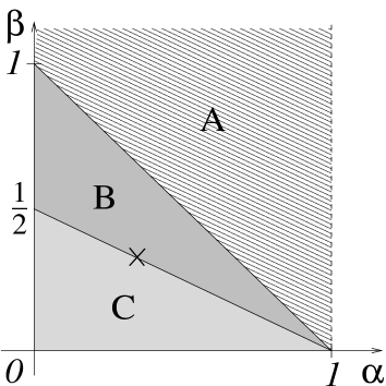
FIG. 2.: Phase diagram of the three different regimes of Lagrangian flow in the time-correlated velocities discussed here. The exponent $\alpha$ is the spatial Hölder exponent and the exponent $\beta$ controls the behavior of correlation time vs scale.

The first idea about the Lagrangian flow in the ensembles (3.1) of quasi-Lagrangian velocities may be gained by comparing the correlation time $\,\tau_{c}(\rho)\,$ to the eddy turnover time $\,\tau_{e}(\rho)=D_{2}^{-1/2}\rho^{1-\alpha}\propto{\rho}/\Sigma(\rho)$.  On the line $\,\alpha+2\beta=1\,$ which, in particular, contains the Kolmogorov point $\,\alpha=\beta={1\over 3}$ (see Fig. 2), both times have the same scale dependence. For $\,\alpha+2\beta<1\,$ (domain  C  on Fig. 2), $\,\tau_{c}\,$ becomes much shorter than $\,\tau_{e}$ at large scales and much longer at small ones. We shall see that in this domain of parameters the pair dispersion should be described at long scales (for $L=\infty)$ by the Kraichnan model with rapidly decorrelating velocities and at short scales by a model with velocities independent of time (frozen). For $\,\alpha+2\beta>1$ (domains  A  and  B  on Fig. 2), the relation between the correlation times is reversed and we could expect that the frozen model controls the large scale dispersion and the decorrelated one governs the short scale behavior. A similar picture underlined the phase diagram in a simple family of scale-invariant shear flows [26]. We shall study the asymptotics of the Lagrangian flow using scale transformations. Such transformations induce a flow in the plane of dimensional parameters of the model whose asymptotics is controlled by fixed points, as in the field theory renormalization group [1]. The perturbative renormalization group has been previously used in [2] to analyze the related scalar advection problem in the family (3.1) of velocity ensembles around $\,(\alpha,\beta)=(-1,1)\,$ and there is some overlap of those results with our conclusions. The much heavier analysis of [2] was concentrated, however, on the aspects of advection related to finer details of the Lagrangian flow, see also [8]. Our point is that the analysis of the Lagrangian dispersion may be performed, at least to at certain extent, in a straightforward and nonperturbative way.

The Kraichnan and the frozen model may be viewed as special limiting cases of the Gaussian velocity ensembles (3.1). The first one, with $\,\xi=2(\alpha+\beta)$, is obtained when $\,D_{2},D_{3}\to\infty\,$ with $\,{2D_{2}\over D_{3}}\equiv D_{1}\,$ kept constant as a consequence of the convergence

$$D_{3}k_{{}_{L}}^{2\beta}\,{\rm e}^{-|t|\,D_{3}k_{{}_{L}}^{2\beta}}\ \mathop{\longrightarrow}\limits_{D_{3}\to\infty}\ 2\,\delta(t)\,.$$ (3.2)

At $\,L=\infty$,  existence of the limit for the correlation functions of $\,\Delta v\,$ requires that $\,\xi<2$,   i.e.  that $\,\alpha+\beta<1$.  Note that the convergence is fast at large wave number $\,k$,  i.e.  at small distances, and for long times, but it becomes slow for short times and, if $\,L=\infty$,  at large distances. The frozen model is obtained by taking $\,D_{3}\to 0\,$ with $\,D_{2}={\rm const}$. In this case,

$${\rm e}^{-D_{3}|t|\,k_{{}_{L}}^{2\beta}}\ \mathop{\longrightarrow}\limits_{D_{3}\to 0}\ 1$$ (3.3)

but the convergence becomes slow at large $\,k$,  i.e.  at small distances, and for long times.

Using the evolution equation (1.4) for the trajectory separation vector, we obtain for the mean rate of growth of the square of pair dispersion:

$${d\over dt}\,\langle\,\rho^{2}(t)\,\rangle\ =\ 2\int\limits_{0}^{t}\Big{\langle}\,\Delta{\mathchoice{{\hbox{\boldmath$\displaystyle v$}}}{{\hbox{\boldmath$\textstyle v$}}}{{\hbox{\boldmath$\scriptstyle v$}}}{{\hbox{\boldmath$\scriptscriptstyle v$}}}}(t,{\mathchoice{{\hbox{\boldmath$\displaystyle\rho$}}}{{\hbox{\boldmath$\textstyle\rho$}}}{{\hbox{\boldmath$\scriptstyle\rho$}}}{{\hbox{\boldmath$\scriptscriptstyle\rho$}}}}(t))\cdot\Delta{\mathchoice{{\hbox{\boldmath$\displaystyle v$}}}{{\hbox{\boldmath$\textstyle v$}}}{{\hbox{\boldmath$\scriptstyle v$}}}{{\hbox{\boldmath$\scriptscriptstyle v$}}}}(s,{\mathchoice{{\hbox{\boldmath$\displaystyle\rho$}}}{{\hbox{\boldmath$\textstyle\rho$}}}{{\hbox{\boldmath$\scriptstyle\rho$}}}{{\hbox{\boldmath$\scriptscriptstyle\rho$}}}}(s))\,\Big{\rangle}\,\,ds\,.$$ (3.4)

Let us start by a naive mean-field-type approximate evaluation of the right hand side in the limit when $\,\rho_{0}\to 0$. Such an evaluation should render correctly the behavior of $\,\langle\,\rho^{2}(t)\,\rangle\,$ in the stochastic regime. It is obtained by rewriting Eq.  (3.4) as

$${d\over dt}\,\langle\,\rho^{2}\,\rangle\ =\ 2\,T\,\,\,\Big{\langle}\,(\Delta{\mathchoice{{\hbox{\boldmath$\displaystyle v$}}}{{\hbox{\boldmath$\textstyle v$}}}{{\hbox{\boldmath$\scriptstyle v$}}}{{\hbox{\boldmath$\scriptscriptstyle v$}}}})^{2}(t,{\mathchoice{{\hbox{\boldmath$\displaystyle\rho$}}}{{\hbox{\boldmath$\textstyle\rho$}}}{{\hbox{\boldmath$\scriptstyle\rho$}}}{{\hbox{\boldmath$\scriptscriptstyle\rho$}}}})\,\Big{\rangle}\,,$$ (3.5)

where

$$T\ =\ {\int\limits_{0}^{t}\Big{\langle}\,\Delta{\mathchoice{{\hbox{\boldmath$\displaystyle v$}}}{{\hbox{\boldmath$\textstyle v$}}}{{\hbox{\boldmath$\scriptstyle v$}}}{{\hbox{\boldmath$\scriptscriptstyle v$}}}}(t,{\mathchoice{{\hbox{\boldmath$\displaystyle\rho$}}}{{\hbox{\boldmath$\textstyle\rho$}}}{{\hbox{\boldmath$\scriptstyle\rho$}}}{{\hbox{\boldmath$\scriptscriptstyle\rho$}}}}(t))\cdot\Delta{\mathchoice{{\hbox{\boldmath$\displaystyle v$}}}{{\hbox{\boldmath$\textstyle v$}}}{{\hbox{\boldmath$\scriptstyle v$}}}{{\hbox{\boldmath$\scriptscriptstyle v$}}}}(s,{\mathchoice{{\hbox{\boldmath$\displaystyle\rho$}}}{{\hbox{\boldmath$\textstyle\rho$}}}{{\hbox{\boldmath$\scriptstyle\rho$}}}{{\hbox{\boldmath$\scriptscriptstyle\rho$}}}}(s))\,\Big{\rangle}\,\,ds\over\Big{\langle}\,(\Delta{\mathchoice{{\hbox{\boldmath$\displaystyle v$}}}{{\hbox{\boldmath$\textstyle v$}}}{{\hbox{\boldmath$\scriptstyle v$}}}{{\hbox{\boldmath$\scriptscriptstyle v$}}}})^{2}(t,{\mathchoice{{\hbox{\boldmath$\displaystyle\rho$}}}{{\hbox{\boldmath$\textstyle\rho$}}}{{\hbox{\boldmath$\scriptstyle\rho$}}}{{\hbox{\boldmath$\scriptscriptstyle\rho$}}}}(t))\,\Big{\rangle}}\,,$$ (3.6)

has, if smaller than $\,t$,  an interpretation of the correlation time of the Lagrangian velocity difference $\,\Delta{\mathchoice{{\hbox{\boldmath$\displaystyle v$}}}{{\hbox{\boldmath$\textstyle v$}}}{{\hbox{\boldmath$\scriptstyle v$}}}{{\hbox{\boldmath$\scriptscriptstyle v$}}}}(t,{\mathchoice{{\hbox{\boldmath$\displaystyle\rho$}}}{{\hbox{\boldmath$\textstyle\rho$}}}{{\hbox{\boldmath$\scriptstyle\rho$}}}{{\hbox{\boldmath$\scriptscriptstyle\rho$}}}}(t))$.  We may try to close Eq.  (3.5) by assuming that $\,T\,$ depends on the mean separation distance $\,\langle\rho^{2}\rangle^{1/2}\,$ the same way as the correlations time $\,\tau_{c}(\rho)\,$ on $\,\rho\,$ if $\,\tau_{c}(\rho)\,$ is smaller than $\,t\,$ or as $\,t\,$ otherwise:

$$T\ \approx\ {\rm min}\{\,{\cal O}(\langle\rho^{2}\rangle^{\beta})\,,\,t\,\}\,.$$ (3.7)

Different domains in the space of parameters correspond to different choices of the minimal value (3.7) for $\,T$.  As for the other term on the right hand side of (3.5), we shall again ignore the velocity dependence of $\,\rho(t)\,$ putting

$$\Big{\langle}\,(\Delta{\mathchoice{{\hbox{\boldmath$\displaystyle v$}}}{{\hbox{\boldmath$\textstyle v$}}}{{\hbox{\boldmath$\scriptstyle v$}}}{{\hbox{\boldmath$\scriptscriptstyle v$}}}})^{2}\,\Big{\rangle}\ \approx\ {\cal O}(\langle\rho^{2}\rangle^{\alpha})$$ (3.8)

Using the above approximations for long times and $L=\infty$, one obtains from (3.5):

$$\hskip 17.07182pt\langle\,\rho^{2}(t)\,\rangle\ \ \approx\ \ \hbox to85.35826pt{${\cal O}(t^{2\over 1-\alpha})$\hfill}{\rm for}\ \ \alpha+2\beta\geq 1\ \ \ \hskip 45.52458pt({\rm domains\ A\ and\ B})\,,$$ (3.9)

$$\hskip 17.07182pt\langle\,\rho^{2}(t)\,\rangle\ \ \approx\ \ \hbox to85.35826pt{${\cal O}(t^{1\over 1-\alpha-\beta})$\hfill}{\rm for}\ \ \alpha+2\beta\leq 1\ \ \ \hskip 45.52458pt({\rm domain\ C})\,.$$ (3.10)

In the same way, we may estimate the short-time behavior in the limit $\,\rho_{0}\to 0\,$ obtaining

$$\langle\,\rho^{2}(t)\,\rangle\ \ \approx\ \ \hbox to85.35826pt{${\cal O}(t^{1\over 1-\alpha-\beta})$\hfill}{\rm for}\,\ \ \hbox to113.81102pt{$\alpha+\beta<1\leq\alpha+2\beta$\hfill}({\rm domain\ B})\,,$$ (3.11)

$$\langle\,\rho^{2}(t)\,\rangle\ \ \approx\ \ \hbox to85.35826pt{${\cal O}(t^{2\over 1-\alpha})$\hfill}{\rm for}\,\ \ \hbox to113.81102pt{$\alpha+2\beta\leq 1$\hfill}({\rm domain\ C})\,.$$ (3.12)

Note that, in agreement with (3.7), it is the smaller exponent that is chosen for large times and the bigger one for short times, a manifestation of a tendency of close trajectories to stay close. The region $\,\alpha+\beta\geq 1\,$ (domain A in Fig. 2) which escapes the short-time estimates has been rigorously analyzed with the Gaussian ensemble (3.1) used to model the Eulerian velocities [14] and was conjectured to correspond to deterministic trajectories. We expect that also in the quasi-Lagrangian model the pair dispersion will concentrate in domain A at $\,\rho=0\,$ when $\,\rho_{0}\to 0$. This is consistent with the divergence of the predicted power in the short-time Richardson law (3.12) when $\,\alpha+\beta\,$ approaches $\,1\,$ from below (i.e.  from the domain B in Fig. 2). A similar divergence occurs in the weakly compressible Kraichnan model when we approach the Lipschitz regime $\,\xi>2\,$ from the non-Lipschitz one $\,\xi<2$.  It signals there the passage from the power law to the exponential separation (2.10) of trajectories.

4 Scaling arguments

The main aim of this note is to substantiate further the above conclusions based on the naive estimates (3.7) and (3.8). We shall also acquire an insight into the behavior of general moments of the pair dispersion and of the exit time and into the extent of the different Lagrangian flow regimes in the ensembles given by Eq.  (3.1). In the study of the long- and short-time behavior of trajectories, it is convenient to consider their rescaled versions $\,{\mathchoice{{\hbox{\boldmath$\displaystyle R$}}}{{\hbox{\boldmath$\textstyle R$}}}{{\hbox{\boldmath$\scriptstyle R$}}}{{\hbox{\boldmath$\scriptscriptstyle R$}}}}_{\mu}(t)=\mu^{-\sigma}{\mathchoice{{\hbox{\boldmath$\displaystyle R$}}}{{\hbox{\boldmath$\textstyle R$}}}{{\hbox{\boldmath$\scriptstyle R$}}}{{\hbox{\boldmath$\scriptscriptstyle R$}}}}(\mu t)\,$ for appropriately chosen $\sigma$.  Since

$${d{\mathchoice{{\hbox{\boldmath$\displaystyle R$}}}{{\hbox{\boldmath$\textstyle R$}}}{{\hbox{\boldmath$\scriptstyle R$}}}{{\hbox{\boldmath$\scriptscriptstyle R$}}}}_{\mu}\over dt}\ =\ {\mathchoice{{\hbox{\boldmath$\displaystyle v$}}}{{\hbox{\boldmath$\textstyle v$}}}{{\hbox{\boldmath$\scriptstyle v$}}}{{\hbox{\boldmath$\scriptscriptstyle v$}}}}_{\mu}(t,{\mathchoice{{\hbox{\boldmath$\displaystyle R$}}}{{\hbox{\boldmath$\textstyle R$}}}{{\hbox{\boldmath$\scriptstyle R$}}}{{\hbox{\boldmath$\scriptscriptstyle R$}}}}_{\mu})\,,$$ (4.1)

for the rescaled velocity $\,{\mathchoice{{\hbox{\boldmath$\displaystyle v$}}}{{\hbox{\boldmath$\textstyle v$}}}{{\hbox{\boldmath$\scriptstyle v$}}}{{\hbox{\boldmath$\scriptscriptstyle v$}}}}_{\mu}(t,{\mathchoice{{\hbox{\boldmath$\displaystyle r$}}}{{\hbox{\boldmath$\textstyle r$}}}{{\hbox{\boldmath$\scriptstyle r$}}}{{\hbox{\boldmath$\scriptscriptstyle r$}}}})=\mu^{1-\sigma}{\mathchoice{{\hbox{\boldmath$\displaystyle v$}}}{{\hbox{\boldmath$\textstyle v$}}}{{\hbox{\boldmath$\scriptstyle v$}}}{{\hbox{\boldmath$\scriptscriptstyle v$}}}}(\mu t,\mu^{\sigma}{\mathchoice{{\hbox{\boldmath$\displaystyle r$}}}{{\hbox{\boldmath$\textstyle r$}}}{{\hbox{\boldmath$\scriptstyle r$}}}{{\hbox{\boldmath$\scriptscriptstyle r$}}}})$, the path $\,{\mathchoice{{\hbox{\boldmath$\displaystyle R$}}}{{\hbox{\boldmath$\textstyle R$}}}{{\hbox{\boldmath$\scriptstyle R$}}}{{\hbox{\boldmath$\scriptscriptstyle R$}}}}_{\mu}(t)$ is a Lagrangian trajectory for $\,{\mathchoice{{\hbox{\boldmath$\displaystyle v$}}}{{\hbox{\boldmath$\textstyle v$}}}{{\hbox{\boldmath$\scriptstyle v$}}}{{\hbox{\boldmath$\scriptscriptstyle v$}}}}_{\mu}$.  There are special cases when the rescaled velocity differences have in the $\,L\to\infty\,$ limit the same distribution as the original ones for an appropriate (and unique) choice of $\,\sigma$. This happens for $\,\sigma={1\over 1-\alpha}\,$ both on the line $\,\alpha+2\beta=1\,$ and in the frozen model and for $\,\sigma={1\over 2-\xi}$ in the Kraichnan ensemble.  We infer that in those cases the pair dispersion PDF $\,{\cal P}\,$ and the exit time one $\,{\cal Q}\,$ are scale-invariant:

$$\mu^{\sigma}\,{\cal P}(\mu^{\sigma}\rho_{0},\mu^{\sigma}\rho;\mu t)\ =\ {\cal P}(\rho_{0},\rho;t)\,,\qquad\mu\,{\cal Q}(\mu t;\mu^{\sigma}\rho_{0},\mu^{\sigma}\rho_{1})\ =\ {\cal Q}(t;\rho_{0},\rho_{1})\,.$$ (4.2)

In particular, in the stochastic regime, the pair dispersion moments $\,\langle\hskip 0.71114pt\rho(t)^{n}\hskip 0.71114pt\rangle$,  if finite in the $\,\rho_{0}\to 0\,$ limit, behave as $\,{\cal O}(t^{n\sigma})\,$ for long times and become proportional to $\,t^{n\sigma}\,$ for all times when $\rho_{0}\to 0$. These conclusions fail in the deterministic regime, as we have already noticed in the Kraichnan model, see Eq.  (2.15). In all regimes, the exit time moments $\,\langle\,t^{n}\,1_{\{t<\infty\}}\,\rangle\,$ (if finite) are proportional to $\,\rho_{0}^{n/\sigma}\,$ if $\,{\rho_{1}\over\rho_{0}}\equiv\gamma\,$ is kept constant.

Out of the line $\,\alpha+2\beta=1$,  the scale invariance of the Lagrangian dispersion is broken but in a predictable way, as we shall see. The crucial observation is that the rescaled velocities $\,{\mathchoice{{\hbox{\boldmath$\displaystyle v$}}}{{\hbox{\boldmath$\textstyle v$}}}{{\hbox{\boldmath$\scriptstyle v$}}}{{\hbox{\boldmath$\scriptscriptstyle v$}}}}_{\mu}(t,{\mathchoice{{\hbox{\boldmath$\displaystyle r$}}}{{\hbox{\boldmath$\textstyle r$}}}{{\hbox{\boldmath$\scriptstyle r$}}}{{\hbox{\boldmath$\scriptscriptstyle r$}}}})\,$ are distributed with the 2-point function (3.1) with $\,D_{i}$ replaced by $\,D_{i,\mu}$ and $\,L\,$ by $\,L_{\mu}$,  where

$$D_{2,\mu}\,=\,\mu^{2[1-(1-\alpha)\sigma]}D_{2}\,\qquad D_{3,\mu}\,=\,\mu^{1-2\beta\sigma}\,D_{3}\,,\qquad L_{\mu}=\mu^{-\sigma}L\,.$$ (4.3)

For $\,\mu\,$ tending to infinity or to zero (i.e.  when exploring the long-time or the short-time behavior of the particle separation), we may choose $\sigma$ so that the distribution of the rescaled velocity differences at $\,L=\infty$ tends to the Kraichnan or to the frozen model ones (with the notable exception of the $\,\mu\to 0\,$ limit in domain A).

Consider first $\,\mu\to\infty$ at $\,L=\infty$.  Taking $\,\sigma={1\over 2(1-\alpha-\beta)}$ fixes the ratio $\,{2D_{2,\mu}\over D_{3,\mu}}\,$ with $\,D_{i,\mu}\to\infty\,$ if $\,\alpha+\beta>1\,$ (domain A in Fig. 2) or if $\,\alpha+2\beta<1$ (domain C in Fig. 2). The latter case leads to a non-singular Kraichnan ensemble of velocity differences with $\,\xi=2(\alpha+\beta)\,$ whereas the former one does not (it would correspond to $\,\xi>2,\ L=\infty$).  We may then expect that

$${\lim\limits_{\mu\to\infty}\ \mu^{\sigma}\,{\cal P}(\mu^{\sigma}\rho_{0},\mu^{\sigma}\rho;\mu t)\ \ \,=\ {\cal P}^{Kr}(\rho_{0},\rho;t)\atop\lim\limits_{\mu\to\infty}\ \mu\,\,{\cal Q}(\mu t;\mu^{\sigma}\rho_{0},\mu^{\sigma}\rho_{1})\,\,\ =\ {\cal Q}^{Kr}(t;\rho_{0},\rho_{1})}\ \bigg{\}}\quad{\rm for}\ \,\sigma={{}_{1}\over{}^{2(1-\alpha-\beta)}}\ \,{\rm and}\,\ \alpha+2\beta<1\,$$ (4.4)

where $\,{\cal P}^{Kr}\,$ and $\,{\cal Q}^{Kr}\,$ pertain to the Kraichnan model with $\,\xi=2(\alpha+\beta)\,$.  This is indeed consistent with the scaling properties of the Kraichnan model dispersion.

Taking $\,\sigma={1\over 1-\alpha}$ fixes $\,D_{2,\mu}$ with $\,D_{3,\mu}\to 0\,$ if $\,\alpha+2\beta>1\,$ (domains A and B in Fig. 2).  We then expect that

$${\lim\limits_{\mu\to\infty}\ \mu^{\sigma}\,{\cal P}(\mu^{\sigma}\rho_{0},\mu^{\sigma}\rho;\mu t)\ \ \,=\ {\cal P}^{fr}(\rho_{0},\rho;t)\atop\lim\limits_{\mu\to\infty}\ \mu\,\,{\cal Q}(\mu t;\mu^{\sigma}\rho_{0},\mu^{\sigma}\rho_{1})\,\,\ =\ {\cal Q}^{\rm fr}(t;\rho_{0},\rho_{1})}\ \bigg{\}}\quad{\rm for}\,\ \sigma={{}_{1}\over{}^{1-\alpha}}\,\ {\rm and}\,\ \alpha+2\beta>1\,,$$ (4.5)

where $\,{\cal P}^{fr}$ and $\,{\cal Q}^{fr}$ stand for the PDF’s of the frozen velocity model with Hölder exponent $\alpha$. Note again the consistency with the scaling properties of the Lagrangian dispersion in the frozen model.

Inquiring about the short-time asymptotics of the trajectory dispersion reverses the asymptotics. We should then have

$${\lim\limits_{\mu\to 0}\ \mu^{\sigma}\,{\cal P}(\mu^{\sigma}\rho_{0},\mu^{\sigma}\rho;\mu t)\ \ \,=\ {\cal P}^{\rm fr}(\rho_{0},\rho;t)\atop\lim\limits_{\mu\to 0}\ \mu\,\,{\cal Q}(\mu t;\mu^{\sigma}\rho_{0},\mu^{\sigma}\rho_{1})\,\,\ =\ {\cal Q}^{fr}(t;\rho_{0},\rho_{1})}\ \bigg{\}}\quad{\rm for}\ \,\sigma={{}_{1}\over{}^{1-\alpha}}\,\ {\rm and}\,\ \alpha+2\beta<1$$ (4.6)

(i.e.  in domain C in Fig. 2) with the same value of the Hölder exponent $\,\alpha$, and

$${\lim\limits_{\mu\to 0}\ \mu^{\sigma}\,{\cal P}(\mu^{\sigma}\rho_{0},\mu^{\sigma}\rho;\mu t)\ =\,{\cal P}^{Kr}(\rho_{0},\rho;t)\atop\lim\limits_{\mu\to 0}\ \mu\,\,{\cal Q}(\mu t;\mu^{\sigma}\rho_{0},\mu^{\sigma}\rho_{1})\,=\,{\cal Q}^{Kr}(t;\rho_{0},\rho_{1})}\ \bigg{\}}\quad{\rm for}\,\ \sigma={{}_{1}\over{}^{2(1-\alpha-\beta)}}\,\ {\rm and}\ \cases{\alpha+\beta<1\,,\cr\alpha+2\beta>1}$$ (4.7)

(i.e.  in domain B in Fig. 2) with $\xi=2(\alpha+\beta)\,$ for the Kraichnan model. Again, this is consistent with the scaling of the limiting PDF’s. In summary, the scale invariance of the statistics of the pair dispersion and of the exit time, although broken away from the $\,\alpha+2\beta=1\,$ line, should be restored at long and short times.

It has to be stressed that the relations (4.4) to (4.7) are conjectural. The PDF’s $\,{\cal P}\,$ and $\,{\cal Q}\,$ are complicated nonlinear functionals of the quasi-Lagrangian velocity statistics and the conjectured relations assume their continuity in an appropriate topology, which is not obvious. In particular, since the convergence of the rescaled velocity covariances to the one of the Kraichnan model is very slow at long distances, there is a potential threat for the corresponding convergence of the rescaled PDF’s $\,{\cal P}(\rho_{0},\rho;t)\,$ and $\,{\cal Q}(t;\rho_{0},\rho_{1})\,$ with $\,\rho_{1}<\rho_{0}\,$ coming from the contribution of trajectories that venture far apart, if such contributions are important. Similarly, the slow convergence to the frozen model at short distances could create problems for the corresponding convergence of the rescaled pair dispersion and exit time PDF’s, for the latter if $\rho_{1}>\rho_{0}$.  Whether such effects invalidate some of the conclusions (4.4) to (4.7) could be, in principle, studied in perturbation theory around the Kraichnan or frozen model. The question of the convergence of rescaled dispersion PDF to the Kraichan model has been recently rigorously studied in [12, 13]. We shall further discuss the non-uniformity of the convergence of the exit time PDF to that of the frozen model in Sect.  6.

An important question concerns the phase diagram of the Lagrangian flow for the model (3.1) of quasi-Lagrangian velocities. As mentioned above, domain A is expected to correspond to the deterministic Lagrangian flow. The rate of separation of close trajectories in this domain (Lyapunov or Richardson flow? locally separating or trapping? locally recurrent or transient?) is also an open problem. Inside domains B and C, we may try to use the conjectured convergence (4.4) to (4.7) of the rescaled pair dispersion and time exit PDF’s to characterize the nature of the Lagrangian flow. This will require even more care since some uniformity of the limits will be needed.

First, we may argue that, inside domains B and C, weak compressibility $\,\wp<{d\over 4(\alpha+\beta)^{2}}\,$ implies that the Lagrangian flow is stochastic. The argument assumes that the dichotomy “deterministic versus stochastic” may be still characterized as in Sect. 2, i.e.  by the behavior of $\,{\cal P}(\rho_{0},\rho;t)\,$ in the limit $\,\rho_{0}\to 0$. It goes as follows. Suppose that the relation (2.2) holds at some point inside B or C (for all $\,t$). Then, obviously, also

$$\lim\limits_{\rho_{0}\to 0}\,\,\mu^{\sigma}\,{\cal P}(\mu^{\sigma}\rho_{0},\mu^{\sigma}\rho;\mu t)\ =\ \delta(\rho)$$ (4.8)

for all $\,\mu$.  We expect the convergence (4.4) in domain C and (4.7) in domain B, both resulting in the Kraichnan model PDF’s, to be uniform at short distances and hence to commute with the $\,\rho_{0}\to 0\,$ limit. We may then infer from Eq.  (4.8) that (2.2) holds also for the limiting Kraichnan PDF so that $\,\wp\geq d/\xi^{2}\,$ where $\,\xi=2(\alpha+\beta)$, which implies the assertion.

The analogous argument may be applied when

$$\lim\limits_{\rho_{0}\to 0}\,\,\int{\cal Q}(t;\rho_{0},\gamma\rho_{0})\,dt\ =\ \lim\limits_{\rho_{0}\to 0}\,\,\int\,\mu\,{\cal Q}(\mu t;\mu^{\sigma}\rho_{0},\mu^{\sigma}\gamma\rho_{0})\,dt\ =\ 1$$ (4.9)

leading to the predictions that inside the domains B and C, the Lagrangian flow is locally trapping if $\,\wp\geq{d\over 4(\alpha+\beta)^{2}}\,$ and locally transient if $\,\wp<{d-2\over 4(\alpha+\beta)}+{1\over 2}$. The first claim seems somewhat more trustable since it does not involve large separations where the convergence to the Kraichnan ensemble is slowed down. Both require additionally that no mass in the exit time PDF escapes to infinity during the $\,\mu$-limits (4.4) and (4.7). This should not pose a problem since convergence to the Kraichnan model becomes very fast at long times.

In the stochastic regime, the convergence (4.4) and (4.7) should imply for the (positive) pair dispersion moments the behavior

$$\langle\,\rho^{n}(t)\,\rangle\ =\ {\cal O}(t^{n\over 2(1-\alpha-\beta)})$$ (4.10)

for long times in domain C and for $\,\rho_{0}\to 0\,$ and short times in domain B, in agreement with the naive mean-field results (3.10) and (3.11). As for the behavior of the moments of the exit time through $\,\gamma\rho_{0}\,$, the relations (4.7) and (4.4) should imply that

$$\langle\,t^{n}\,1_{\{t<\infty\}}\,\rangle\ =\ {\cal O}(\rho_{0}^{2n(1-\alpha-\beta)})$$ (4.11)

in domain B for small $\,\rho_{0}\,$ and in domain C for large ones, irrespectively of the character of the Lagrangian flow. Similarly, we should obtain in domain B the convergence

$$\lim\limits_{\mu\to 0}\,\,\int f(t)\,\,{\cal Q}(t;\mu^{\sigma}\rho_{0},\mu^{\sigma}\gamma\rho_{0})\,dt\ =\ f(0)\int{\cal Q}^{Kr}(t;\rho_{0},\rho_{1})\,dt$$ (4.12)

characteristic of the Richardson flow in our terminology.

Similar use of the conjectured convergences (4.5) and (4.6) to the frozen model PDF’s in order to argue about the Lagrangian flow dichotomies and the evolution of dispersion and exit times moments poses two problems. First is the poor knowledge of the flow behavior in the frozen model, see, however, Sect. 5. Second, even more serious one, is the non-uniform nature of the convergence that becomes slow at small distances and long times. It is still plausible, however, that the convergence (4.5) is uniform enough as to imply that

$$\langle\,\rho^{n}(t)\,\rangle\ =\ {\cal O}(t^{n\over(1-\alpha)})$$ (4.13)

for long times and for sufficiently high $\,n\,$ in the stochastic regime in domains A and B.  Similarly, relations (4.5) and (4.6) may still imply that for sufficiently negative moments,

$$\langle\,t^{n}\,\rangle\ =\ {\cal O}(\rho_{0}^{n(1-\alpha)})$$ (4.14)

in domains A and B for large $\,\rho_{0}\,$ and in domain C for small ones, see Sect.  6. The same way, the convergence (4.12) should still hold in domain C for test functions $\,f\,$ decaying fast at infinity and $\,Q^{Kr}\,$ replaced by $\,{\cal Q}^{fr}$.

Summarizing, we predict, with various level of confidence, that the Lagrangian flow is

deterministic

in domain A

stochastic, Richardson, locally transient

in domains B and C  for $\,\wp<{d-2\over{}^{4(\alpha+\beta)}}+{1\over 2}\,$,

stochastic, Richardson

in domains B and C  for $\,{d-2\over{}^{4(\alpha+\beta)}}+{1\over 2}\leq\wp<{d\over 4(\alpha+\beta)^{2}}\,$,

Richardson, locally trapping

in domains B and C  for $\,\wp\geq{d\over 4(\alpha+\beta)^{2}}\,$.

The degree of confidence of the predictions depends on which of relations (4.4) to (4.7) was used in the argument and with what uniformity assumptions. The predictions are consistent with the intuition that increase of the compressibility degree $\,\wp\,$ enhances the trapping of the fluid particles. It will be interesting to confirm (or infirm) them by further analytic arguments and by numerical simulations. Note that, in particular, we expect that in domains B and C the incompressible Lagrangian flow is stochastic, Richardson and locally transient, and that, if the dimension $\,d\geq 4$,  it stays such, whatever compressibility.

5 One-dimensional frozen ensemble

The frozen model was left out from the discussion of the phase diagram in the last section. Our arguments were based mainly on the convergence of the rescaled velocity ensemble (3.1) to the Kraichnan model and such convergence is, of course, absent for the frozen model. One may expect appearance of discontinuity in the character of the Lagrangian flow in the frozen model limit $\,D_{3}\to 0\,$ which is is very non-uniform at short distances and long times, leading to a strong enhancement of trapping. This effect will be analyzed in next Section. Here we shall try to find out what happens in the frozen velocities which, in general, are the hard to analyze. One case where some analytic results may be obtained is the one-dimensional Gaussian model with the Hölder exponent $\alpha={1\over 2}$ and 2-point function

$$\langle v(x)\,v(y)\rangle\ =\ \int{{\rm e}^{ik(x-y)}\over k^{2}+L^{-2}}\,{dk\over 2\pi}\ =\ {{}_{1}\over{}^{2}}{L}\,{\rm e}^{-|x-y|/L}\,,$$ (5.1)

where, for simplicity, we have set $\,D_{2}=1\,$ (what may be always achieved by rescaling $\,v\mapsto\sqrt{D_{2}}\,v$). A simplifying feature of this case, studied already in [29], is that $v(x)$ forms a stationary Markov (Ornstein-Uhlenbeck) process with the generator

$${\cal L}\ =\ -{{}_{1}\over{}^{2}}{{}_{d^{2}}\over{}^{dv^{2}}}+{{}_{v}\over{}^{L}}{{}_{d}\over{}^{dv}}$$ (5.2)

corresponding to the Focker-Planck harmonic oscillator Hamiltonian

$${\cal H}\ =\ {\rm e}^{-{v^{2}\over 2L}}{\cal L}\,\,{\rm e}^{\,v^{2}\over 2L}\ =\ -{{}_{1}\over{}^{2}}{{}_{d^{2}}\over{}^{dv^{2}}}+{{}_{v^{2}}\over{}^{2L^{2}}}-{{}_{1}\over{}^{2L}}\,.$$ (5.3)

The velocity $\,v(x)\,$ with fixed $\,x\,$ is distributed according to the invariant measure of the process

$$d\nu(v)\ =\ {{}_{1}\over{}^{\sqrt{\pi L}}}\,\,{\rm e}^{-{v^{2}\over L}}\,dv\,.$$ (5.4)

The transition probabilities of the process are

$$p(v_{0},v;t)\,dv\, = \,{\rm e}^{-t\,{\cal L}}(v_{0},v)\,dv\ =\ {{}_{1}\over{}^{\sqrt{\pi L(1-{\rm e}^{-2t/L})}}}\,\,{\rm e}^{-{({\rm e}^{-t/L}v_{{}_{0}}-v)^{2}\over L(1-{\rm e}^{-2t/L})}}\,dv\,.$$ (5.5)

In the limit $L\to\infty$, the velocity difference $\,\Delta v(x)=v(x)-v(0)\,$ becomes the one-dimensional two-sided Brownian motion $\,w(x)$.  The quasi-Lagrangian Eq.  (1.4) for the trajectory separation takes then the form of the steepest descent equation

$${d\rho\over dt}\ =\ \,w(\rho)\ =\ -{d\over d\rho}\phi(\rho)\,.$$ (5.6)

in the potential $\,\phi(x)=-\,\int\limits_{0}^{x}w(y)\,dy$. The solution $\,\rho(t)\,$ slides to the bottom of the potential well in which the initial point $\,\rho_{0}=\rho(0)\,$ is situated, i.e. to the closest zero $\,\rho_{+}$ of $\,w(\rho)\,$ to the right of $\,\rho_{0}$ if $\,w(\rho_{0})>0\,$ or $\,\rho_{-}$ to the left of $\,\rho_{0}$ is $\,w(\rho_{0})<0$.  The only difference with the case of smooth potential with wells approximately quadratic around typical minima, is that, as we show below, the solution will arrive to the bottom of the well in a finite rather than infinite time. This is due to the roughness of the Brownian motion. After arriving at the bottom, the solution will stay locked there in subsequent times.

We may restrict ourselves to the case $\,\rho_{0}>0$. Suppose also that $\,w(\rho_{0})>0$. The first value $\,\rho_{+}$ to the right of $\,\rho_{0}$ such that $\,w(\rho_{+})=0$ is finite with probability one. The time $\,t_{+}$ that the solution $\,\rho(t)\,$ of Eq.  (5.6) starting at $\,\rho_{0}$ at time zero takes to reach $\,\rho_{+}$ is

$$t_{+}\ =\ \int\limits_{\rho_{0}}^{\rho_{+}}{d\rho\over w(\rho)}\,.$$ (5.7)

Let us compute the expectation $\,\langle\,t_{+}\,1_{\{w(\rho_{0})>0,\,\rho_{+}\leq\rho_{2}\}}\rangle\,$ of times $\,t_{+}$ over the Brownian paths $\,w(\rho)\,$ such that $\,w(\rho_{0})>0\,$ and $\,\rho_{+}\leq\rho_{2}\,$ for certain $\,\rho_{2}>\rho_{0}$. It is equal to

$$\int\limits_{\rho_{0}}^{\rho_{2}}d\rho\int\limits_{0}^{\infty}{\rm e}^{-{w_{0}^{2}\over 2\rho_{0}}}{{}_{dw_{0}}\over{}^{\sqrt{2\pi\rho_{0}}}}\int\limits_{0}^{\infty}\Big{(}{\rm e}^{-{(w_{0}-w)^{2}\over 2(\rho-\rho_{0})}}-\,{\rm e}^{-{(w_{0}+w)^{2}\over 2(\rho-\rho_{0})}}\Big{)}{{}_{dw}\over{}^{\sqrt{2\pi(\rho-\rho_{0})}\,w}}\int\limits_{0}^{\infty}{\rm e}^{-{(w+w_{2})^{2}\over 2(\rho_{2}-\rho)}}{{}_{2\,dw_{2}}\over{}^{\sqrt{2\pi(\rho_{2}-\rho)}}}\,.$$ (5.8)

The origin of this formula is straightforward. The probability that $\,w(\rho_{0})\,$ belongs to $\,[w_{0},w_{0}+dw_{0}]\,$ is $\,{\rm e}^{-{w_{0}^{2}\over 2\rho_{0}}}{dw_{0}\over\sqrt{2\pi\rho_{0}}}$.  The one that $\,w(\rho)\,$ belongs to $\,[w,w+dw]\,$ without passing through zero between $\,\rho_{0}\,$ and $\,\rho\,$ is $\,\Big{(}{\rm e}^{-{(w_{0}-w)^{2}\over 2(\rho-\rho_{0})}}-\,{\rm e}^{-{(w_{0}+w)^{2}\over 2(\rho-\rho_{0})}}\Big{)}{dw\over\sqrt{2\pi(\rho-\rho_{0})}}$, given that $\,w(\rho_{0})=w_{0}$, (it is expressed by the heat kernel with the Dirichlet condition at $\,w=0$).  Finally, the last integral on the right hand side of (5.8) is equal to the probability that the Brownian trajectory crosses zero between $\,\rho\,$ and $\,\rho_{2}$, given that $\,w(\rho)=w$.  In Appendix  1 we show that

$$\langle\,t_{+}\,1_{\{w(\rho_{0})>0,\,\rho_{+}\leq\rho_{2}\}}\rangle\ \leq\ {C_{+}}\,\rho_{0}^{1/2}\,\ln{{}_{\rho_{2}}\over{}^{\rho_{0}}}\,,$$ (5.9)

where $\,C_{+}\,$ is a dimensionless constant. This proves that the time $\,t_{+}\,$ is almost surely finite although the unrestricted mean $\,\langle\,t_{+}\,1_{\{w(\rho_{0})>0\}}\,\rangle$,  given by the $\,\rho_{2}\to\infty\,$ limit of (5.8) under which the last integral on the right hand side tends to one, diverges. The divergence is due to the contribution of the Brownian paths that travel far before falling back to zero. In the Ornstein-Uhlenbeck process with $\,L<\infty$,  the weight of such paths is suppressed and it is not difficult to show that $\,\langle\,t_{+}\,1_{\{w(\rho_{0})>0\}}\,\rangle\,$ is finite then.

Similarly, let $\,w(\rho_{0})<0$ and $\,0\leq\rho_{-}<\rho_{0}$ be the first value to the left of $\,\rho_{0}$ such that $\,w(\rho_{-})=0$. The time $\,t_{-}$ that the solution $\,\rho(t)\,$ of Eq.  (5.6) starting at $\,\rho_{0}$ at time zero takes to reach $\,\rho_{-}$ is given by Eq.  (5.7) with $\,t_{+}$ replaced by $\,t_{-}$ and $\,\rho_{+}$ by $\,\rho_{-}$.  The expectation value $\,\langle\,t_{-}\,1_{\{w(\rho_{0})<0\}}\,\rangle\,$ is given by

$$-\int\limits_{0}^{\rho_{0}}d\rho\int\limits_{-\infty}^{0}{\rm e}^{-{w^{2}\over 2\rho}}{{}_{dw}\over{}^{\sqrt{2\pi\rho}\,\,w}}\int\limits_{-\infty}^{0}\Big{(}{\rm e}^{-{(w-w_{0})^{2}\over 2(\rho_{0}-\rho)}}-\,{\rm e}^{-{(w+w_{0})^{2}\over 2(\rho_{0}-\rho)}}\Big{)}{{}_{dw_{0}}\over{}^{\sqrt{2\pi(\rho_{0}-\rho)}}}$$ (5.10)

which is easily seen to be finite, e.g.  by bounding the last integral by $\,\sqrt{2\over\pi(\rho_{0}-\rho)}\,|w|$. We infer that

$$\langle\,t_{-}\,1_{\{w(\rho_{0})<0\}}\,\rangle\ =\ {C_{-}}\,\rho_{0}^{1/2}\,,$$ (5.11)

where $\,C_{-}$ is another dimensionless constant.

A  Exit time

As for the exit time that the process $\,\rho(t)\,$ takes to grow from $\,\rho_{0}\,$ to $\,\rho_{1}>\rho_{0}$,  it is finite if and only if $\,\rho(t)\,$ is not stuck at a zero $\,\rho_{\pm}<\rho_{1}$ of $\,w(\rho)$, i.e.  if $\,w\,$ is positive on the interval $\,[\rho_{0},\rho_{1})$.  It is then given by the formula

$$t\ =\ \int\limits_{\rho_{0}}^{\rho_{1}}{d\rho\over w(\rho)}\,.$$ (5.12)

The probability that $\,t<\infty\,$ is given by

$$\langle\,1_{\{t<\infty\}}\,\rangle\ =\ \int\limits_{0}^{\infty}{\rm e}^{-{w_{0}^{2}\over 2\rho_{0}}}{{}_{dw_{0}}\over{}^{\sqrt{2\pi\rho_{0}}}}\int\limits_{0}^{\infty}\Big{(}{\rm e}^{-{(w_{0}-w_{1})^{2}\over 2(\rho_{1}-\rho_{0})}}-\,{\rm e}^{-{(w_{0}+w_{1})^{2}\over 2(\rho_{1}-\rho_{0})}}\Big{)}{{}_{dw_{1}}\over{}^{\sqrt{2\pi(\rho_{1}-\rho_{0})}}}\,.$$ (5.13)

Note that the last expression depends only on $\,{\rho_{1}\over\rho_{0}}$,  is smaller than $\,1/2\,$ and tends to zero when $\,\rho_{0}\to 0\,$ with $\,\rho_{1}$ fixed.  With the complementary probability, the solution $\,\rho(t)\,$ starting from $\,\rho_{0}>0\,$ will never reach $\,\rho_{1}$,  i.e.  the exit time $\,t\,$ is infinite.  The averages of positive powers of the exit time constraint to be finite are expressed by the relation

$$\langle\,t^{n}\,1_{\{t<\infty\}}\,\rangle\ =\ n!\int\limits_{\rho_{0}\leq\rho^{\prime}\leq\dots\leq\rho^{(n)}\leq\rho_{1}}d\rho^{\prime}\cdots d\rho^{(n)}\ \int\limits_{0}^{\infty}{\rm e}^{-{w_{0}^{2}\over 2\rho_{0}}}{{}_{dw_{0}}\over{}^{\sqrt{2\pi\rho_{0}}}}\hskip 56.9055pt\,\,$$ (5.14)

$$\cdot\ \prod\limits_{i=1}^{n}\int\limits_{0}^{\infty}\Big{(}{\rm e}^{-{(w^{(i-1)}-w^{(i)})^{2}}\over 2(\rho^{(i)}-\rho^{(i-1)})}-\,{\rm e}^{-{(w^{(i-1)}+w^{(i)})^{2}}\over 2(\rho^{(i)}-\rho^{(i-1)})}\Big{)}{{}_{dw^{(i)}}\over{}^{\sqrt{2\pi(\rho^{(i)}-\rho^{(i-1)})}\,\,w^{(i)}}}\,\,\,$$ (5.15)

$$\cdot\ \int\limits_{0}^{\infty}\Big{(}{\rm e}^{-{(w^{(n)}-w_{1})^{2}\over 2(\rho_{1}-\rho^{(n)})}}-\,{\rm e}^{-{(w^{(n)}+w_{1})^{2}\over 2(\rho_{1}-\rho^{(n)})}}\Big{)}{{}_{dw_{1}}\over{}^{\sqrt{2\pi(\rho_{1}-\rho^{(n)})}}}$$ (5.16)

with $\,\rho^{(0)}\equiv\rho_{0}\,$ and $\,w^{(0)}\equiv w_{0}$.  It is easy to show that the expression on the right hand side is finite. Indeed, bounding the last integral by $\,\sqrt{2\over\pi(\rho_{1}-\rho^{(n)})}w^{(n)}\,$ as in estimating (5.10) and proceeding further the same way, we obtain the inequality

$$\langle\,t^{n}\,1_{\{t<\infty\}}\,\rangle\ \leq\ {{}_{1}\over{}^{\pi}}\left({{}_{2}\over{}^{\pi}}\right)^{n/2}\sqrt{\rho_{0}}\,\ n!\int\limits_{\rho_{0}\leq\rho^{\prime}\leq\dots\leq\rho^{(n)}\leq\rho_{1}}{{}_{d\rho^{\prime}\cdots d\rho^{(n)}}\over{}^{\sqrt{(\rho^{\prime}-\rho_{0})\cdots(\rho_{1}-\rho^{(n)})}}}\,\,$$ (5.17)

$$\leq\ {{}_{2^{n}}\over{}^{\sqrt{2\pi}}}\,{{}_{n!}\over{}^{(n-1)!!}}\,({{}_{\rho_{1}}\over{}^{\rho_{0}}}-1)^{{}^{n-1\over 2}}\,\rho_{0}^{{}^{n\over 2}}\,,$$ (5.18)

where the last line results from the inductive calculation of the $\rho^{(i)}$ integrals. As a consequence of the scaling properties of the right hand side of Eq.  (5.16),

$$\langle\,t^{n}\,1_{\{t<\infty\}}\,\rangle\ =\ {C_{n}}\,\rho_{0}^{n/2}\ =\ C_{n}\,\tau_{e}^{n}\,$$ (5.19)

where $\,C_{n}\,$ are dimensionless constants depending on the ratio $\,\gamma={\rho_{1}\over\rho_{0}}>1\,$ and $\,\tau_{e}=(\rho_{0}/D_{2})^{1/2}\,$ is the eddy turnover time at scale $\,\rho_{0}\,$ (recalled that we have set $D_{2}=1$ above).

The bounds (5.18), which respect the above scaling, imply that the characteristic function $\,\langle\,{\rm e}^{i\omega t}\,1_{\{t<\infty\}}\,\rangle\,$ is entire in $\omega$ and that the large $\,t\,$ decay of the PDF $\,{\cal Q}(t;\rho_{0},\rho_{1})\,$ is at least $\,\propto{\rm e}^{-{\cal O}(t^{2})}$.  Due to Eq.  (5.12), the characteristic function may be expressed by the path integral

$$\langle\,{\rm e}^{i\omega t}\,1_{\{t<\infty\}}\,\rangle\,\ =\ {{}_{1}\over{}^{\cal N}}\,\int\limits_{0}^{\infty}{\rm e}^{-{w_{0}^{2}\over 2\rho_{0}}}{{}_{dw_{0}}\over{}^{\sqrt{2\pi\rho_{0}}}}\int{\rm e}^{\,\int\limits_{\rho_{0}}^{\rho_{1}}\left({i\omega\over w(\rho)}\,-\,{1\over 2}{\dot{w}}^{2}(\rho)\right)d\rho}\,{\cal D}w$$ (5.20)

over the paths $\,[\rho_{0},\rho_{1}]\ni\rho\mapsto w(\rho)\in(0,\infty)\,$ such that $\,w(\rho_{0})=w_{0}$,  with $\,{\cal N}\,$ being an appropriate normalization factor. The expression permits to evaluate the large $\,|\omega|$-behavior along the positive imaginary axis of $\,\omega\,$ by the semi-classical calculation. The extremal trajectory $\,w(\rho)\,$ describes a motion of a unit mass particle climbing up in the potential $\,-{1\over w}\,$ until a total stop. It satisfies the equation

$${{}_{\sin{\varphi_{0}}}\over{}^{\cos^{3}{\varphi_{0}}}}\left(\varphi+\sin{\varphi}\cos{\varphi}\right)\ =\ {{}_{\rho_{1}}\over{}^{\rho_{0}}}-{{}_{\rho}\over{}^{\rho_{0}}}$$ (5.21)

for $\,\cos^{2}{\varphi}={w(\rho)\over w(\rho_{1})}$, $\,\cos^{2}{\varphi_{0}}={w(\rho_{0})\over w(\rho_{1})}\,$ and $\,\varphi\,$ between zero and $\,\varphi_{0}<{\pi\over 2}$.  In particular, $\,\varphi_{0}\,$ is determined by Eq.  (5.21) with $\,\varphi=\varphi_{0}\,$ and $\,\rho=\rho_{0}$.  It depends only on the ratio $\,{\rho_{1}\over\rho_{0}}$.  The action of the classical trajectory is $\,S_{0}=|\omega|^{2/3}\rho_{0}^{1/3}s_{0}\,$ with a dimensionless constant $\,s_{0}={3\varphi_{0}\,\sin^{1/3}{\varphi_{0}}\over 2^{1/3}\cos{\varphi_{0}}}\,$ growing with the $\,{\rho_{1}\over\rho_{0}}$.  The decay $\,\sim{\rm e}^{-S_{0}}\,$ of the characteristic function along the positive imaginary axis corresponds to the small $\,t\,$ behavior $\,\sim{\rm e}^{-{4\over 27}\,\rho_{0}\,s_{0}^{3}\,t^{-2}}={\rm e}^{-{4\over 27}\,s_{0}^{3}\,(\tau_{e}/t)^{2}}\,$ of the exit time PDF $\,{\cal Q}(t;\rho_{0},\rho_{1})\,$ (up to powers of $\,t$).  One could expect that for short times the trajectories move almost ballistically:

$$\rho(t)\ \simeq\ \rho_{0}+w(\rho_{0})t$$ (5.22)

which would give $\,t\simeq{\rho_{1}-\rho_{0}\over w(\rho_{0})}\,$ and a short time tale $\,\sim{\rm e}^{-{(\rho_{1}-\rho_{0})^{2}\over 2\rho_{0}}\,t^{-2}}\,$ of the exit time PDF. This reproduces well the power of $\,t\,$ in the exponential but not the coefficient. The latter, divided by $\,\rho_{0}$,  agrees only to the order $\,({\rho_{1}\over\rho_{0}}-1)^{2}$ with the correct expression $\,{4\over 27}s_{0}^{3}$.

For $\,\omega\,$ on the imaginary axis, the path-integral on the right hand side of Eq.  (5.20) may be re-expressed in the operator language via the Feynman-Kac formula. Using also the invariance of the Brownian motion under the scale transformations $\,w(x)\mapsto|\omega|^{-1}w(|\omega|^{2}x)$,  we obtain the identity

$$\langle\,{\rm e}^{i\omega t}\,1_{\{t<\infty\}}\,\rangle\,\ =\ \int\limits_{0}^{\infty}{\rm e}^{-{w_{0}^{2}\over 2|\omega|^{2}\rho_{0}}}{{}_{dw_{0}}\over{}^{\sqrt{2\pi\rho_{0}}\,|\omega|}}\int\limits_{0}^{\infty}{\rm e}^{-|\omega|^{2}(\rho_{1}-\rho_{0}){\cal K}_{{}_{\pm}}}(w_{0},w_{1})\,dw_{1}\,,$$ (5.23)

where the operator

$${\cal K}_{\pm}\ =\ -{{}_{1}\over{}^{2}}{{}_{d^{2}}\over{}^{dw^{2}}}\pm{{}_{1}\over{}^{w}}$$ (5.24)

on the interval $\,[0,\infty)\,$ is a 1-dimensional Schrödinger operator with Dirichlet boundary condition at zero. The signs pertain to the positive or negative imaginary $\,\omega$-axis and result in a repulsive or an attractive potential, respectively. An explicit expression for the kernel of the exponential of $\,{\cal K}_{-}$,  see Appendix  2, shows the growth of the characteristic function for $\,\omega=-i|\omega|\,$ dominated by the lowest bound state contribution $\,\sim{\rm e}^{\,-|\omega|^{2}(\rho_{1}-\rho_{0})E_{0}}\,$ with $\,E_{0}=-{1\over 2}$.  This implies the decay $\,\sim{\rm e}^{-{1\over(\rho_{1}-\rho_{0})}\,t^{2}}={\rm e}^{-{1\over\gamma-1}\,(t/\tau_{e}(\rho_{0}))^{2}}\,$ of the PDF $\,{\cal Q}(t;\rho_{0},\rho_{1})\,$ for large $\,t$.

The above analytic predictions may be used to validate the numerical method to be applied later for the cases $\alpha\neq 1/2$, where such rigorous results are not available. The velocity field is generated by using a straightforward Fourier method, i.e. generating the Fourier modes by a standard Gaussian random number generator and transforming back to real space by Fast Fourier Transform. The resolution which we used was $2^{20}$. The initial separation is set at $20,000$ and we measure the PDF of the time taken to reach $5$ times the initial separation. The curve is shown in Fig. 3. The agreement with the superposed predictions indicates that the choice of the resolution and the initial separation are appropriate to avoid contamination by periodicity and/or discretization effects.

FIG. 3.: The PDF of the exit times for the frozen flow with $\alpha=1/2$. The dotted curves are the analytical predictions at small and large times, respectively.

The time in which $\,\rho(t)\,$ decreases from $\,\rho_{0}\,$ to a positive value $\,\rho_{1}<\rho_{0}\,$ is finite and still determined by Eq.  (5.12) if and only if $\,w<0\,$ on the interval $\,(\rho_{1},\rho_{0}]$.  It is easy to see that

$${\cal Q}(t;\rho_{0},\rho_{1})\ =\ {\cal Q}(t;\rho_{1},\rho_{0})$$ (5.25)

since for $\,\rho_{1}<\rho_{0}\,$ the characteristic function $\,\langle\,{\rm e}^{i\omega t}\,1_{\{t<\infty\}}\,\rangle\,$ is given by the expression (5.20) with $\,\rho_{0}\,$ and $\,\rho_{1}\,$ interchanged.

The scaling property (4.2) with $\,\sigma=2\,$ and the fact that the exit time is infinite with a positive probability depending on $\,{\rho_{1}\over\rho_{0}}\,$ imply that

$$\lim\limits_{\rho_{0}\to 0}\,\,{\cal Q}(t;\rho_{0},\gamma\rho_{0})=c(\gamma)\,\delta(t)$$ (5.26)

for any positive $\,\gamma\not=1\,$ with $\,0<c(\gamma)<1$.  It follows that the Lagrangian flow is Richardson. locally trapping and locally transient in the terminology of Sect. 2A.

B  Pair dispersion

The pair dispersion in the model is closely related to the exit time. The reason is that the solution $\,\rho(t)\,$ of Eq.  (5.6) never changes direction. As a result, the solution that starts at $\,\rho_{0}\,$ at time zero satisfies $\,\rho(t)\geq\rho_{1}\geq\rho_{0}\,$ or $\,\rho(t)\leq\rho_{1}\leq\rho_{0}\,$ if and only if it exits through $\,\rho_{1}\,$ in time shorter than $\,t$.  It follows that

$$\int\limits_{\rho_{1}}^{\infty}{\cal P}(\rho_{0},\rho;t)\,d\rho\ =\ \int\limits_{0}^{t}{\cal Q}(s;\rho_{0},\rho_{1})\,ds\qquad{\rm for}\quad\rho_{1}\geq\rho_{0}\,,$$ (5.27)

$$\int\limits_{0}^{\rho_{1}}{\cal P}(\rho_{0},\rho;t)\,d\rho\ =\ \int\limits_{0}^{t}{\cal Q}(s;\rho_{0},\rho_{1})\,ds\qquad{\rm for}\quad\rho_{1}\leq\rho_{0}\,\,$$ (5.28)

or that

$${\cal P}(\rho_{0},\rho;t)\ =\ \mp\,\partial_{\rho}\int\limits_{0}^{t}{\cal Q}(s;\rho_{0},\rho)\,ds\qquad{\rm for}\quad\rho\,\,{{}_{{}_{>}}\atop{}^{{}^{<}}}\,\hskip 0.71114pt\rho_{0}\,.$$ (5.29)

The right hand side of Eq.  (5.27) is bounded by $\,\int\limits_{0}^{\infty}{\cal Q}(s;\rho_{0},\rho_{1})\,ds\,$ which tends to zero when $\,\rho_{0}\to 0\,$ for $\,\rho_{1}>0\,$ fixed,  see Eq.  (5.13). It follows that

$$\lim\limits_{\rho_{0}\to 0}\ {\cal P}(\rho_{0},\rho;t)\ =\ \delta(\rho)\,,$$ (5.30)

in agreement with the fact that the trajectories are determined by the initial condition. Hence the Lagrangian flow is deterministic. Note the important difference with the phase V of the Kraichnan model, see Fig. 1. There the trapping effects resulted in the coalescence of fluid particles signaled by the singular form (2.13) of the pair dispersion PDF. With the use of symmetry (5.25), the left hand side of Eq.  (5.28) may be bounded by $\,\int\limits_{0}^{\infty}{\cal Q}(s;\rho_{1},\rho_{0})\,ds\,$ and hence tends to zero when $\,\rho_{1}\to 0\,$ for fixed $\,\rho_{0}>0$.  As a result, the PDF $\,{\cal P}(\rho_{0},\rho;t)\,$ cannot have a contribution proportional to $\,\delta(\rho)\,$ for $\,\rho_{0}>0$.  It is, instead, regular in $\,\rho$.   The reason is that in the quasi-Lagrangian model of particle separation (5.6), the solutions $\,\rho(t)\,$ are trapped with probability 1 at positive zeros of $\,w\,$ (there is an infinity of such zeros) and never arrive at $\,\rho=0$. This seems to be an artifact of the frozen one-dimensional model but it serves as a warning that the behavior of trajectories in the time-correlated velocities may be richer than what was observed for the Kraichnan model, with a possible occurrence of phase

VI.  deterministic, Richardson, locally trapping, locally transient

characterized by a combination of properties that did not occur in the time-decorrelated model.

C  Case with $\,\alpha\not={1\over 2}$

Several of the features analytically established for the one-dimensional frozen model with the Hölder exponent $\,\alpha={1\over 2}\,$ may be generalized to the case of general $\,\alpha\,$ in the interval $\,(0,1)$,  although the absence of the Markov property in the process $\,v(x)\,$ makes the arguments more difficult, see [21]. In the limit $\,L\to\infty$,  the equation for the trajectory separation still has the form (5.6) with $\,w(x),\ x\geq 0,\,$ being (upon a right choice of the normalization constant $D_{2}$) the two-sided fractional Brownian motion (fBm), i.e.  the Gaussian process with mean zero and 2-point function

$$\langle w(x)\,w(y)\rangle\ =\ {{}_{1}\over{}^{2}}(x^{2\alpha}+y^{2\alpha}-|x-y|^{2\alpha})\ \equiv\ G(x,y)\,$$ (5.31)

for $\,x,\,y\geq 0$.  The 2-point function (5.31) is a kernel of a positive operator on the half-axis $\,[0,\infty)\,$ that we shall denote by $\,G$. Note the scale invariance under $\,w(x)\mapsto\mu^{-\alpha}w(\mu x)\,$ of the fBm. The basic result of [27] asserts that the probability that $\,w(x)<w_{0}\,$ for $\,w_{0}>0\,$ and all $\,x\,$ in the interval $\,(0,\rho_{0})\,$ behaves like $\,{\cal O}((\rho_{0}w_{0}^{-1/\alpha})^{1-\alpha})\,$ for large values of $\,\rho_{0}w_{0}^{-1/\alpha}$.   Similarly as for the Brownian motion, the fBm lives on continuous trajectories and has zeros in any interval $\,(0,\rho_{0})\,$ or $\,(\rho_{0},\infty)$. One may again prove that, with probability 1, the solution $\,\rho(t)\,$ of Eq.  (5.6) starting at any $\,\rho_{0}>0\,$ arrives in finite time at the closest zero $\,\rho_{\pm}\,$ to the right or left of $\,\rho_{0}$,  see [21].

As in the case $\,\alpha={1\over 2}$,  the exit time $\,t\,$ through $\,\rho_{1}>\rho_{0}\,$ is finite if and only if $\,w>0\,$ on the interval $\,[\rho_{0},\rho_{1})\,$ and the probability $\,\langle\,1_{\{t<\infty\}}\,\rangle\,$ of such an event depends only on $\,{\rho_{1}\over\rho_{0}}\,$ and tends to zero when $\,\rho_{0}\to 0$. It should be again possible to extract the behaviors of the exit time PDF $\,{\cal Q}(t;\rho_{0},\rho_{1})\,$ for large and small time by looking at the large $\,|\omega|\,$ behavior of

$$\langle\,{\rm e}^{\pm|\omega|t}\,1_{\{t<\infty\}}\,\rangle\ =\ \langle\,{\rm e}^{\pm|\omega|\int\limits_{\rho_{0}}^{\rho_{1}}{d\rho\over w(\rho)}}\,1_{\{w>0\ {\rm on}\ [\rho_{0},\rho_{1})\}}\,\rangle\,,$$ (5.32)

where the last expectation is with respect to the Gaussian measure of the fBm $\,w$.  For the

negative sign, this expression should be still dominated for large $\,|\omega|\,$ by the semi-classical contribution $\,\sim{\rm e}^{-S_{0}}$.  The classical trajectory $\,w(\rho)=|\omega|^{1/3}\rho_{0}^{(1+2\alpha)/3}(Gu)({\rho\over\rho_{0}}),$  where $\,u\,$ is a function that does not vanish only on the interval $\,(1,{\rho_{1}\over\rho_{0}})\,$ and such that

$$u\ =\ (Gu)^{-2}$$ (5.33)

there. Note that it follows that $\,w(\rho)>0\,$ for $\,\rho>0\,$ since $\,G(x,y)>0\,$ except for $\,x,y=0$.  The action of the classical trajectory is $\,S_{0}=|\omega|^{2/3}\,\rho_{0}^{2(1-\alpha)/3}\,s_{0}\,\,$ for

$$s_{0}\ =\ \int\limits_{1}^{\rho_{1}/\rho_{0}}\Big{[}{{}_{1}\over{}^{(Gu)(x)}}\,+\,{{}_{1}\over{}^{2}}\,u(x)\,(Gu)(x)\Big{]}\,dx\,.$$ (5.34)

Such a semi-classical dominance implies again the small time tail $\,\,\sim{\rm e}^{-{4\over 27}\,\rho_{0}^{2(1-\alpha)}\,s_{0}^{3}\,t^{-2}}={\rm e}^{-{\cal O}((\tau_{e}/t)^{2})}\,$ of the exit time PDF $\,{\cal Q}(t;\rho_{0},\rho_{1})\,$ (with the eddy turnover time $\,\tau_{e}=D_{2}^{-1/2}\rho_{0}^{1-\alpha}$).

With the use of the scale invariance of the fBm, one may also absorb the $\,|\omega|$-dependence of the characteristic function into the length of the $\,\rho$-interval in Eq.  (5.32):

$$\langle\,{\rm e}^{\pm|\omega|t}\,1_{\{t<\infty\}}\,\rangle\ =\ \langle\,{\rm e}^{\pm\int\limits_{\rho^{\prime}_{0}}^{\rho^{\prime}_{1}}{d\rho\over w(\rho)}}\,1_{\{w>0\ {\rm on}\ [\rho^{\prime}_{0},\rho^{\prime}_{1})\}}\,\rangle\,,$$ (5.35)

where $\,\rho^{\prime}_{i}=|\omega|^{1\over 1-\alpha}\rho_{i}$.  For the positive sign in Eq.  (5.35) and $\,\alpha={1\over 2}$,  we have used the Feynman-Kac formula in order to extract the extensive behavior of the right hand side for large $\,|\omega|$.  For other values of $\,\alpha\in(0,1)\,$ such a formula is not available but the expectation (5.35) may be viewed as the partition function of a one-dimensional continuous spin system with long-range 2-spin interactions decaying as $\,distance^{-2(1+\alpha)}\,$ and with partially confining (as opposed to the case with negative sign) single-spin potential. It is plausible that the extensive behavior of the partition function $\,\,\sim\,{\rm e}^{-|\omega|^{{}_{1}\over{}^{1-\alpha}}(\rho_{1}-\rho_{0})E_{0}}\,\,$ for large $\,|\omega|\,$ with free energy density $\,E_{0}<0\,$ persists for such systems. Such a behavior would result in the long-time tail $\,\,\sim\,{\rm e}^{-\alpha({1-\alpha\over|(\rho_{1}-\rho_{0})E_{0}|})^{(1-\alpha)/\alpha}\,t^{1/\alpha}}={\rm e}^{-{\cal O}((t/\tau_{e})^{1/\alpha})}\,$ of the PDF $\,{\cal Q}(t;\rho_{0},\rho_{1})$.  The validity of this prediction is confirmed by Figs. 4 and 5 where we present the PDF’s of the exit times for the two cases $\alpha=0.4$ and $0.75$. The numerical simulations are realized by the same method previously validated in the case $\alpha=1/2$.

The statistics of the time of exit through $\,\rho_{1}<\rho_{0}\,$ is again obtained from that for $\,\rho_{1}>\rho_{0}\,$ by interchanging $\,\rho_{0}\,$ and $\,\rho_{1}$ and the pair dispersion PDF is still given by Eq.  (5.29). The remarks about the phase VI type behavior of Lagrangian flow carry over from the case $\,\alpha={1\over 2}$.

FIG. 4.: The PDF of the exit times for the 1$d$ frozen velocities with $\alpha=0.4$. The dotted curve is a fit of the form ${\rm e}^{-{\rm const.}\,t^{1/\alpha}}$.

FIG. 5.: The PDF of the exit times for the 1$d$ frozen velocities with $\alpha=3/4$. The solid curve is a fit of the form ${\rm e}^{-{\rm const.}\,t^{1/\alpha}}$. Since the curve gives the visual impression of an exponential decay, we also plot in the inset $\ln|\ln({\cal Q}(t;\rho_{0},\rho_{1}))|$ vs $\log t$ and compare the slopes $0.75$ and $1$ to validate the former.

6 Effect of long time velocity correlations

The presence of permanent trapping of trajectories in one-dimensional frozen ensemble, leading to events with infinite exit time through $\,\rho_{1}=\gamma\rho_{0}$,  should also occur in higher-dimensional frozen ensembles obtained by setting $\,D_{3}=0\,$ in Eq.  (3.1). It is plausible that, at least in the presence of compressibility, the sets of velocities trapping trajectories in a given region have positive probability. If, however, one reintroduces finite temporal correlations of velocities by taking positive $\,D_{3}\,$ in (3.1), the particles will eventually be released from traps after the time evolution changes the velocity field configuration, i.e.  after time of order $\,\tau_{c}(\rho)=D_{3}^{-1}\rho^{2\beta}\,$ for traps of size $\,\rho$.  If for $\,D_{3}>0\,$ the exit times are finite so that $\,\int\limits_{0}^{\infty}{\cal Q}(t)\,dt=1$,  then the missing probability $\,1-\int\limits_{0}^{\infty}{\cal Q}(t)\,dt>0\,$ for $\,D_{3}=0\,$ should be built from the long-time tails of $\,{\cal Q}\,$ at positive $\,D_{3}$,  as the latter is taken to zero. We may then expect that, loosely speaking, for fixed $\,\rho_{0}$, $\,\gamma\,$ and $\,D_{2}$,

$${\cal Q}(t;\rho_{0},\gamma\rho_{0})\ \approx\tau_{c}^{-1}\,{\cal Q}^{\infty}(t/\tau_{c},\gamma)\qquad{\rm for}\quad t/\tau_{c}\gg 1\,.$$ (6.1)

with $\,\tau_{c}=\tau_{c}(\rho_{0})\,$ and the function $\,{\cal Q}^{\infty}\,$ having a (Poissonian) exponential tail. Let us concentrate on the one-dimensional situation where the frozen exit-time PDF is expected to have a stretched exponential tail $\,\sim{\rm e}^{-{\cal O}((t/\tau_{e})^{1/\alpha})}\,$ with the scale set by the eddy turnover time $\,\tau_{e}=D_{2}^{-1/2}\rho_{0}^{1-\alpha}$.  Note that the latter attains the value of order $\,\tau_{c}^{-1}\,$ for $\,t=\tau^{\prime}\,$ with $\,\tau^{\prime}/\tau_{e}={\cal O}((\ln(\tau_{c}/\tau_{e}))^{\alpha})={\cal O}(|\ln D_{3}|^{\alpha})$. The “minimal” scenario would be that the frozen PDF passes into the form of (6.1) around $\,t=\tau^{\prime}$.  More precisely, we may postulate the convergence

$${\cal Q}(t;\rho_{0},\gamma\rho_{0})\,\,1_{\{t<\tau^{\prime}\}} \mathop{\longrightarrow}\limits_{D_{3}\to 0} \ \quad{\cal Q}^{fr}(t;\rho_{0},\gamma\rho_{0})$$ (6.2)

$$\tau_{c}\,\,{\cal Q}(s\tau_{c};\rho_{0},\gamma\rho_{0})\,\,1_{\{s\geq\tau^{\prime}/\tau_{c}\}} \mathop{\longrightarrow}\limits_{D_{3}\to 0} \ \quad{\cal Q}^{\infty}(s;\gamma)$$ (6.4)

in a strong enough sense. The above relations imply that the large exit time behavior becomes self-similar for small $\,D_{3}$,  with the characteristic scale equal to $\tau_{c}$,  with no intermediate regime between the frozen type behavior and the self-similar tail. It is also possible that a different intermediate regime sets in between times of order $\,\tau^{\prime}\,$ and $\,\tau_{c}$, with $\,\tau^{\prime}\,$ depending differently on $\,D_{3}$.

The minimal scenario would make explicit the large $\,t\,$ non-uniformity of the conjectured convergence of the exit time PDF’s, see (4.5) and (4.6). Recall that the conjecture was based on the scaling relation that may be rewritten as the identity

$$\rho_{0}^{1-\alpha}\,{\cal Q}(\rho_{0}^{1-\alpha}t;\rho_{0},\gamma\rho_{0})|_{{}_{D_{3}}}\ =\ {\cal Q}(t;1,\gamma)|_{{}_{D_{3}(\rho_{0})}}$$ (6.5)

for $\,D_{3}(\rho_{0})=\rho_{0}^{1-\alpha-2\beta}D_{3}\,$ and $\,D_{2}\,$ unchanged, see (4.3). When $\,\rho_{0}\to\infty\,$ in domain A and B and $\,\rho_{0}\to 0\,$ in domain C then $\,D_{3}(\rho_{0})\to 0\,$ so that we fall into the situation considered in the scenario (LABEL:scen). The latter becomes then the assertion that

$$\rho_{0}^{1-\alpha}\,{\cal Q}(\rho_{0}^{1-\alpha}t,\rho_{0},\gamma\rho_{0})\,\,1_{\{t<\tau^{\prime}(\rho_{0})\}} \mathop{\longrightarrow}\limits_{\rho_{0}\to{\infty\atop 0}} \ \quad{\cal Q}^{fr}(t;1,\gamma)$$ (6.6)

$$D_{3}^{-1}\rho_{0}^{2\beta}\,{\cal Q}(D_{3}^{-1}\rho_{0}^{2\beta};\rho_{0},\gamma\rho_{0})\,\,1_{\{s\geq D_{3}(\rho_{0})\tau^{\prime}(\rho_{0})\}} \mathop{\longrightarrow}\limits_{\rho_{0}\to{\infty\atop 0}} \ \quad{\cal Q}^{\infty}(s;\gamma)$$ (6.8)

for $\,\tau^{\prime}(\rho_{0})={\cal O}(|\ln\rho_{0}|^{\alpha})$.

One of the consequences of such a limiting behavior would be a bifractal scaling with $\,\rho_{0}\to\infty\,$ or $\,\rho_{0}\to 0\,$ of the moments of the exit time. Indeed,

$$\int\limits_{0}^{\infty}t^{n}\,\,{\cal Q}(t;\rho_{0},\gamma\rho_{0})\,dt\ =\ \rho_{0}^{(1-\alpha)n}\int\limits_{0}^{\tau^{\prime}(\rho_{0})}t^{n}\,\rho_{0}^{1-\alpha}\,{\cal Q}(\rho_{0}^{1-\alpha}t;\rho_{0},\gamma\rho_{0})\,dt\,\,$$ (6.9)

$$+\ D_{3}^{-n}\rho_{0}^{2\beta n}\int\limits_{D_{3}(\rho_{0})\tau^{\prime}(\rho_{0})}^{\infty}s^{n}\,D_{3}^{-1}\,\rho_{0}^{2\beta}\,{\cal Q}(D_{3}^{-1}\,\rho_{0}^{2\beta}s;\rho_{0},\gamma\rho_{0})\,ds\,.$$ (6.10)

In the regime of extreme values of $\,\rho_{0}$,  the first term on the right hand side behaves like $\,\,\rho_{0}^{(1-\alpha)n}\int\limits_{0}^{\infty}t^{n}\,{\cal Q}^{fr}(t;1,\gamma)\,dt\,\,$ if we assume (LABEL:scen') with a sufficiently strong convergence. Similarly the second term would behave like $\,\,D_{3}^{-n}\rho_{0}^{2\beta n}\int\limits_{D_{3}(\rho_{0})\tau^{\prime}(\rho_{0})}^{\infty}s^{n}\,{\cal Q}^{\infty}(s;\gamma)\,ds$.  If $\,Q^{\infty}(s,\gamma)$ is integrable at zero, the first term dominates for negative $\,n\,$ and the second one for positive $\,n\,$ when it behaves as $\,{\cal O}(\rho_{0}^{2\beta n})$.  The “minimal” scenario (LABEL:scen) would then imply that

$$\langle\,t^{n}\,\rangle\ =\ \cases{\hbox to85.35826pt{${\cal O}(\rho_{0}^{n(1-\alpha)})$\hfill}{\rm for}\quad n\leq 0\,,\cr\cr\hbox to85.35826pt{${\cal O}(\rho_{0}^{2\beta n})$\hfill}{\rm for}\quad n\geq 0}$$ (6.11)

for large $\,\rho_{0}\,$ in domain A and B and for small $\,\rho_{0}\,$ in domain C. Such a bifractal behavior is, of course, consistent with the earlier conjecture (4.14).  The missing probability in the frozen case would be given by $\,\int\limits_{0}^{\infty}{\cal Q}^{\infty}(s;\gamma)\,ds$.  Even in the presence of an intermediate regime in the exit time PDF, the scaling (6.11) should set in for $\,|n|\gg 1$.  The convexity (concavity) of the large (small) $\,\rho_{0}\,$ exponent as a function of $\,n$,  together with its vanishing at $\,n=0$,  would then impose the behavior (6.11) for all $\,n$.

We have tested the scenario (LABEL:scen) numerically. The one-dimensional velocity field with temporal correlations was obtained again using the Fourier method. Each Fourier mode $v_{k}(t)$ was generated by integrating the corresponding Uhlenbeck-Ornstein differential equation:

$${dv_{k}(t)}\ =\ -{v_{k}(t)\over\tau(k)}dt\,+\,\Big{(}{2E(k)\over\tau(k)}\Big{)}^{{}^{1/2}}dW(t)\,,$$ (6.12)

where $\,\tau(k)\,$ scales as $\,k^{-2\beta}\,$, the energy spectrum of the field is denoted by $\,E(k)\propto k^{-1-2\alpha}\,$ and $\,dW(t)\,$ is a standard Brownian motion. The stochastic differential equations (6.12) were integrated by using a simple Euler scheme of order ${1\over 2}$ [22].

FIG. 6.: The PDF of the exit times for the flow with $\,\alpha=0.75\,$ and $\,\beta=0.3\,$ at six initial separations $\,\rho_{0}=400,800,1200,1500,1800,2100$.  The resolution is $32768$.

    

FIG. 7.: The same PDF as in the previous figure but plotted now as $\,\rho_{0}^{1-\alpha}{\cal Q}\,$ vs $\,\rho_{0}^{\alpha-1}t\,$ to display the collapse at small exit times.

  

FIG. 8.: The same PDF as in the previous figure but plotted now as $\,\rho_{0}^{2\beta}{\cal Q}\,$ vs $\,\rho_{0}^{-2\beta}t\,$ to display the collapse at large exit times.

The parameters of the flow where $\,\alpha=0.75\,$ and $\,\beta=0.3$. The exit times for six different initial separations was measured. Their PDF’s $\,{\cal Q}(t;\rho_{0},1.05\rho_{0})\,$ are shown in Fig. 6. According to (LABEL:scen'), by plotting $\,\rho_{0}^{1-\alpha}{\cal Q}$ versus $\rho_{0}^{\alpha-1}t\,$ all the curves should collapse at small exit times, as confirmed in Fig. 7. Furthermore, the prediction (LABEL:scen') at large exit times is verified in Fig. 8 by collapsing the long-time parts of the curves by plotting $\,\rho_{0}^{2\beta}\,{\cal Q}\,$ versus $\,\rho_{0}^{-2\beta}t$.  Note that the curves for the two smallest values of $\,\rho_{0}\,$ are not collapsing, in agreement with the previous arguments predicting that the asymptotic behavior sets in at large $\,\rho_{0}$’s. The simulations are consistent with the absence of an intermediate regime but do not really allow to exclude such a possibility.

7 Eulerian Gaussian velocities:  sweeping effects

Let us discuss how the Lagrangian flow changes if the Gaussian velocity ensemble 3.1 is used to model the Eulerian velocities rather than the quasi-Lagrangian ones. As already mentioned, the main difference is that, unlike for the Kraichnan model, the separation of two trajectories is not any more a function of velocity differences only and it is strongly influenced by large-scale eddies or the so called sweeping. This effect grows with growing integral scale $\,L\,$ and we shall attempt to study its large $\,L\,$ asymptotics. It seems to be stronger for small values of $\,\beta$,  i.e.  for velocities that are almost frozen at small distances.

The r.m.s. value of velocity in the ensemble (3.1) is proportional to $\,L^{\alpha}$,  i.e.  it becomes large for large $\,L$.  On the other hand, the r.m.s. equal-time velocity differences on scales much smaller than $\,L\,$ are of the order $\,distance^{\alpha}$.  In particular, on the scales $\sim L^{\alpha}\,$ they are of the order $\,L^{\alpha^{2}}\ll L^{\alpha}$.   Rewriting the trajectory equation (1.1) as

$$\mathchoice{{\hbox{\boldmath$\displaystyle R$}}}{{\hbox{\boldmath$\textstyle R$}}}{{\hbox{\boldmath$\scriptstyle R$}}}{{\hbox{\boldmath$\scriptscriptstyle R$}}}(t)\ =\ \int\limits_{0}^{t}\mathchoice{{\hbox{\boldmath$\displaystyle v$}}}{{\hbox{\boldmath$\textstyle v$}}}{{\hbox{\boldmath$\scriptstyle v$}}}{{\hbox{\boldmath$\scriptscriptstyle v$}}}(s,\mathchoice{{\hbox{\boldmath$\displaystyle 0$}}}{{\hbox{\boldmath$\textstyle 0$}}}{{\hbox{\boldmath$\scriptstyle 0$}}}{{\hbox{\boldmath$\scriptscriptstyle 0$}}})\,ds\ +\ \int\limits_{0}^{t}[\mathchoice{{\hbox{\boldmath$\displaystyle v$}}}{{\hbox{\boldmath$\textstyle v$}}}{{\hbox{\boldmath$\scriptstyle v$}}}{{\hbox{\boldmath$\scriptscriptstyle v$}}}(s,\mathchoice{{\hbox{\boldmath$\displaystyle R$}}}{{\hbox{\boldmath$\textstyle R$}}}{{\hbox{\boldmath$\scriptstyle R$}}}{{\hbox{\boldmath$\scriptscriptstyle R$}}}(s))-\mathchoice{{\hbox{\boldmath$\displaystyle v$}}}{{\hbox{\boldmath$\textstyle v$}}}{{\hbox{\boldmath$\scriptstyle v$}}}{{\hbox{\boldmath$\scriptscriptstyle v$}}}(s,\mathchoice{{\hbox{\boldmath$\displaystyle 0$}}}{{\hbox{\boldmath$\textstyle 0$}}}{{\hbox{\boldmath$\scriptstyle 0$}}}{{\hbox{\boldmath$\scriptscriptstyle 0$}}})]\,ds\,,$$ (7.1)

we may expect that, for fixed $\,t$,  the first integral is of the order $\,L^{\alpha}\,$ and the second of the order $\,L^{\alpha^{2}}\ll L^{\alpha}$. For bounded times, the first integral should then give the term of the order $\,L^{\alpha}\,$ of the solution and the second one, with $\,\mathchoice{{\hbox{\boldmath$\displaystyle R$}}}{{\hbox{\boldmath$\textstyle R$}}}{{\hbox{\boldmath$\scriptstyle R$}}}{{\hbox{\boldmath$\scriptscriptstyle R$}}}(s)\,$ replaced by the approximation $\,\sim L^{\alpha}$,  the term of the order $\,L^{\alpha^{2}}$.  More precisely, let us observe that the Gaussian process with the components $\,L^{-\alpha}\mathchoice{{\hbox{\boldmath$\displaystyle v$}}}{{\hbox{\boldmath$\textstyle v$}}}{{\hbox{\boldmath$\scriptstyle v$}}}{{\hbox{\boldmath$\scriptscriptstyle v$}}}(t,\mathchoice{{\hbox{\boldmath$\displaystyle 0$}}}{{\hbox{\boldmath$\textstyle 0$}}}{{\hbox{\boldmath$\scriptstyle 0$}}}{{\hbox{\boldmath$\scriptscriptstyle 0$}}})\,$ and $\,L^{-\alpha^{2}}[\mathchoice{{\hbox{\boldmath$\displaystyle v$}}}{{\hbox{\boldmath$\textstyle v$}}}{{\hbox{\boldmath$\scriptstyle v$}}}{{\hbox{\boldmath$\scriptscriptstyle v$}}}(t,L^{\alpha}\mathchoice{{\hbox{\boldmath$\displaystyle r$}}}{{\hbox{\boldmath$\textstyle r$}}}{{\hbox{\boldmath$\scriptstyle r$}}}{{\hbox{\boldmath$\scriptscriptstyle r$}}})-\mathchoice{{\hbox{\boldmath$\displaystyle v$}}}{{\hbox{\boldmath$\textstyle v$}}}{{\hbox{\boldmath$\scriptstyle v$}}}{{\hbox{\boldmath$\scriptscriptstyle v$}}}(t,\mathchoice{{\hbox{\boldmath$\displaystyle 0$}}}{{\hbox{\boldmath$\textstyle 0$}}}{{\hbox{\boldmath$\scriptstyle 0$}}}{{\hbox{\boldmath$\scriptscriptstyle 0$}}})]\,$ converges in law when $\,L\to\infty\,$ to the $\,t$-independent Gaussian process $\,(\mathchoice{{\hbox{\boldmath$\displaystyle v$}}}{{\hbox{\boldmath$\textstyle v$}}}{{\hbox{\boldmath$\scriptstyle v$}}}{{\hbox{\boldmath$\scriptscriptstyle v$}}}_{0},\,\mathchoice{{\hbox{\boldmath$\displaystyle w$}}}{{\hbox{\boldmath$\textstyle w$}}}{{\hbox{\boldmath$\scriptstyle w$}}}{{\hbox{\boldmath$\scriptscriptstyle w$}}}(\mathchoice{{\hbox{\boldmath$\displaystyle r$}}}{{\hbox{\boldmath$\textstyle r$}}}{{\hbox{\boldmath$\scriptstyle r$}}}{{\hbox{\boldmath$\scriptscriptstyle r$}}}))\,$ with the 2-point functions

$$\hbox to79.6678pt{$\langle\,\mathchoice{{\hbox{\boldmath$\displaystyle v$}}}{{\hbox{\boldmath$\textstyle v$}}}{{\hbox{\boldmath$\scriptstyle v$}}}{{\hbox{\boldmath$\scriptscriptstyle v$}}}_{0}\,\mathchoice{{\hbox{\boldmath$\displaystyle v$}}}{{\hbox{\boldmath$\textstyle v$}}}{{\hbox{\boldmath$\scriptstyle v$}}}{{\hbox{\boldmath$\scriptscriptstyle v$}}}_{0}\,\rangle$\hfill}=\ \ D_{2}\int{1\over k_{1}^{d+2\alpha}}\,{d\mathchoice{{\hbox{\boldmath$\displaystyle k$}}}{{\hbox{\boldmath$\textstyle k$}}}{{\hbox{\boldmath$\scriptstyle k$}}}{{\hbox{\boldmath$\scriptscriptstyle k$}}}\over(2\pi)^{d}}\,,$$ (7.2)

$$\hbox to79.6678pt{$\langle\,\mathchoice{{\hbox{\boldmath$\displaystyle w$}}}{{\hbox{\boldmath$\textstyle w$}}}{{\hbox{\boldmath$\scriptstyle w$}}}{{\hbox{\boldmath$\scriptscriptstyle w$}}}(\mathchoice{{\hbox{\boldmath$\displaystyle r$}}}{{\hbox{\boldmath$\textstyle r$}}}{{\hbox{\boldmath$\scriptstyle r$}}}{{\hbox{\boldmath$\scriptscriptstyle r$}}})\,\mathchoice{{\hbox{\boldmath$\displaystyle w$}}}{{\hbox{\boldmath$\textstyle w$}}}{{\hbox{\boldmath$\scriptstyle w$}}}{{\hbox{\boldmath$\scriptscriptstyle w$}}}(\mathchoice{{\hbox{\boldmath$\displaystyle r$}}}{{\hbox{\boldmath$\textstyle r$}}}{{\hbox{\boldmath$\scriptstyle r$}}}{{\hbox{\boldmath$\scriptscriptstyle r$}}}^{\prime})\,\rangle$\hfill}=\ \ D_{2}\int{(1-{\rm e}^{i\mathchoice{{\hbox{\boldmath$\displaystyle k$}}}{{\hbox{\boldmath$\textstyle k$}}}{{\hbox{\boldmath$\scriptstyle k$}}}{{\hbox{\boldmath$\scriptscriptstyle k$}}}\cdot\mathchoice{{\hbox{\boldmath$\displaystyle r$}}}{{\hbox{\boldmath$\textstyle r$}}}{{\hbox{\boldmath$\scriptstyle r$}}}{{\hbox{\boldmath$\scriptscriptstyle r$}}}})(1-{\rm e}^{-i\mathchoice{{\hbox{\boldmath$\displaystyle k$}}}{{\hbox{\boldmath$\textstyle k$}}}{{\hbox{\boldmath$\scriptstyle k$}}}{{\hbox{\boldmath$\scriptscriptstyle k$}}}\cdot\mathchoice{{\hbox{\boldmath$\displaystyle r$}}}{{\hbox{\boldmath$\textstyle r$}}}{{\hbox{\boldmath$\scriptstyle r$}}}{{\hbox{\boldmath$\scriptscriptstyle r$}}}^{\prime}})\over k^{d+2\alpha}}\,{d\mathchoice{{\hbox{\boldmath$\displaystyle k$}}}{{\hbox{\boldmath$\textstyle k$}}}{{\hbox{\boldmath$\scriptstyle k$}}}{{\hbox{\boldmath$\scriptscriptstyle k$}}}\over(2\pi)^{d}}\,,$$ (7.3)

$$\hbox to79.6678pt{$\langle\,\mathchoice{{\hbox{\boldmath$\displaystyle v$}}}{{\hbox{\boldmath$\textstyle v$}}}{{\hbox{\boldmath$\scriptstyle v$}}}{{\hbox{\boldmath$\scriptscriptstyle v$}}}_{0}\,\mathchoice{{\hbox{\boldmath$\displaystyle w$}}}{{\hbox{\boldmath$\textstyle w$}}}{{\hbox{\boldmath$\scriptstyle w$}}}{{\hbox{\boldmath$\scriptscriptstyle w$}}}(\mathchoice{{\hbox{\boldmath$\displaystyle r$}}}{{\hbox{\boldmath$\textstyle r$}}}{{\hbox{\boldmath$\scriptstyle r$}}}{{\hbox{\boldmath$\scriptscriptstyle r$}}})\,\rangle$\hfill}=\ \ 0\,\,.$$ (7.4)

Note the independence of $\,\mathchoice{{\hbox{\boldmath$\displaystyle v$}}}{{\hbox{\boldmath$\textstyle v$}}}{{\hbox{\boldmath$\scriptstyle v$}}}{{\hbox{\boldmath$\scriptscriptstyle v$}}}_{0}\,$ and $\,\mathchoice{{\hbox{\boldmath$\displaystyle w$}}}{{\hbox{\boldmath$\textstyle w$}}}{{\hbox{\boldmath$\scriptstyle w$}}}{{\hbox{\boldmath$\scriptscriptstyle w$}}}(\mathchoice{{\hbox{\boldmath$\displaystyle r$}}}{{\hbox{\boldmath$\textstyle r$}}}{{\hbox{\boldmath$\scriptstyle r$}}}{{\hbox{\boldmath$\scriptscriptstyle r$}}})$.  It is then natural to conjecture that the following convergence in law takes place:

$$\hbox to130.88284pt{$L^{-\alpha}\mathchoice{{\hbox{\boldmath$\displaystyle R$}}}{{\hbox{\boldmath$\textstyle R$}}}{{\hbox{\boldmath$\scriptstyle R$}}}{{\hbox{\boldmath$\scriptscriptstyle R$}}}(t)$\hfill}\ \mathop{\longrightarrow}\limits_{L\to\infty}\qquad\mathchoice{{\hbox{\boldmath$\displaystyle v$}}}{{\hbox{\boldmath$\textstyle v$}}}{{\hbox{\boldmath$\scriptstyle v$}}}{{\hbox{\boldmath$\scriptscriptstyle v$}}}_{0}t\,,$$ (7.5)

$$\hbox to130.88284pt{$L^{-\alpha^{2}}\Big{[}\mathchoice{{\hbox{\boldmath$\displaystyle R$}}}{{\hbox{\boldmath$\textstyle R$}}}{{\hbox{\boldmath$\scriptstyle R$}}}{{\hbox{\boldmath$\scriptscriptstyle R$}}}(t)-\int\limits_{0}^{t}\mathchoice{{\hbox{\boldmath$\displaystyle v$}}}{{\hbox{\boldmath$\textstyle v$}}}{{\hbox{\boldmath$\scriptstyle v$}}}{{\hbox{\boldmath$\scriptscriptstyle v$}}}(s,\mathchoice{{\hbox{\boldmath$\displaystyle 0$}}}{{\hbox{\boldmath$\textstyle 0$}}}{{\hbox{\boldmath$\scriptstyle 0$}}}{{\hbox{\boldmath$\scriptscriptstyle 0$}}})\,ds\Big{]}$\hfill}\ \mathop{\longrightarrow}\limits_{L\to\infty}\qquad\int\limits_{0}^{t}\mathchoice{{\hbox{\boldmath$\displaystyle w$}}}{{\hbox{\boldmath$\textstyle w$}}}{{\hbox{\boldmath$\scriptstyle w$}}}{{\hbox{\boldmath$\scriptscriptstyle w$}}}(\mathchoice{{\hbox{\boldmath$\displaystyle v$}}}{{\hbox{\boldmath$\textstyle v$}}}{{\hbox{\boldmath$\scriptstyle v$}}}{{\hbox{\boldmath$\scriptscriptstyle v$}}}_{0}s)\,ds\,.$$ (7.6)

In the frozen case or if $\,\alpha\leq\beta\,$ or $\,\alpha>\beta>\alpha(1-\alpha)$,  the limits describe the leading terms in the single trajectory statistics for large $\,L$.  For $\beta\leq\alpha(1-\alpha)$,   one should also take into account the term coming from $\,\int\limits_{0}^{t}[\mathchoice{{\hbox{\boldmath$\displaystyle v$}}}{{\hbox{\boldmath$\textstyle v$}}}{{\hbox{\boldmath$\scriptstyle v$}}}{{\hbox{\boldmath$\scriptscriptstyle v$}}}(s,\mathchoice{{\hbox{\boldmath$\displaystyle 0$}}}{{\hbox{\boldmath$\textstyle 0$}}}{{\hbox{\boldmath$\scriptstyle 0$}}}{{\hbox{\boldmath$\scriptscriptstyle 0$}}})-\mathchoice{{\hbox{\boldmath$\displaystyle v$}}}{{\hbox{\boldmath$\textstyle v$}}}{{\hbox{\boldmath$\scriptstyle v$}}}{{\hbox{\boldmath$\scriptscriptstyle v$}}}(0,\mathchoice{{\hbox{\boldmath$\displaystyle 0$}}}{{\hbox{\boldmath$\textstyle 0$}}}{{\hbox{\boldmath$\scriptstyle 0$}}}{{\hbox{\boldmath$\scriptscriptstyle 0$}}})]\,ds\,$ which is of order $\,L^{\alpha-\beta}$. The dominant term of order $\,L^{\alpha}\,$ in $\,\mathchoice{{\hbox{\boldmath$\displaystyle R$}}}{{\hbox{\boldmath$\textstyle R$}}}{{\hbox{\boldmath$\scriptstyle R$}}}{{\hbox{\boldmath$\scriptscriptstyle R$}}}(t)\,$ describes the ballistic motion with the random velocity of the largest scale eddies that sweep the Lagrangian particle along. In Appendix 3 we prove convergence (7.5) in the frozen one-dimensional model with $\,\alpha={1\over 2}$.

How does the presence of large scale $\,L\,$ in Eulerian velocities influence the Lagrangian particle separation? Let us try to understand this in the one-dimensional frozen model. We shall consider two particle trajectories $\,x(t)\,$ and $\,x(t)+\rho_{0}\,$  starting at time zero at zero and  $\rho_{0}>0$,  respectively, and we shall try to estimate the behavior of their separation $\,\rho(t)$.  First notice that $\,\rho(t)\geq 0$, i.e. the order of the particles on the line will never change. For large $\,L$,  the dominant events are when the velocities of the particles and at the points between them are all of the order $\,L^{\alpha}\,$ and of the same sign during the time interval $\,(0,t)$.  Let us suppose that they are positive, see Fig. 9 (the case of negative velocities can be treated in a symmetric way). The crucial fact resulting from the one-dimensional geometry is the magic identity

$$\int\limits_{0}^{\rho_{0}}{{d\rho}\over{v(\rho)}}\ \ =\ \int\limits_{x(t)}^{x(t)+\rho(t)}{{d\rho}\over{v(\rho)}}\,.$$ (7.7)

The left hand side is the time $\,\Delta t\,$ that the first particle takes to reach the initial position of the second one. The best way to understand the above identity is by releasing the second particle after the delay $\,\Delta t\,$ so that both particles move subsequently together. The delay changes nothing in the movement of the second particle since the velocity field is frozen. The delayed particle will then be at position $\,x(t)\,$ at time $\,t\,$ (together with the first particle) and at position $\,x(t)+\rho(t)\,$ at time $\,t+\Delta t$. But the right hand side of Eq.  (7.7) is the time that the second particle takes to move from $\,x(t)\,$ to $\,x(t)+\rho(t)$.

FIG. 9.: Positions of two right-moving particles in $1d$ frozen velocity

Hence the identity which may be also proven more formally by noticing that the time derivative of its right hand side vanishes. Writing for large $\,L$

$$x(t)\ =\ L^{\alpha}v_{0}t\,+\ {\cal O}(L^{\alpha^{2}})\,,\qquad v(x(t))\ =\ L^{\alpha}v_{0}\,+\,L^{\alpha^{2}}w(v_{0}t)\,+\ {\cal O}(L^{\alpha^{3}})\,,$$ (7.8)

see relations (7.5) and (7.6), and anticipating that $\,\rho(t)={\cal O}(1)$,  Eq.  (7.7) may be approximated as

$${{\rho_{0}}\over{L^{\alpha}v_{0}}}\ =\ {{\rho(t)}\over{L^{\alpha}v_{0}+L^{\alpha^{2}}w(v_{0}t)}}\,+\,{\cal O}(L^{\alpha^{3}-2\alpha})$$ (7.9)

from which we infer that

$$\rho(t)-\rho_{0}\ =\ L^{\alpha^{2}-\alpha}\rho_{0}\,v_{0}^{-1}w(v_{0}t)\ +\ {\cal O}(L^{\alpha^{3}-\alpha})\,.$$ (7.10)

The process $\,w(x)\,$ is the fBm with the 2-point function (5.31) (up to normalization). The precise conjecture would then assert the convergence in law

$$L^{\alpha(1-\alpha)}\,[\rho(t)-\rho_{0}]\ \quad\mathop{\longrightarrow}\limits_{L\to\infty}\ \quad\rho_{0}\,v_{0}^{\alpha-1}\,w(t)\,.$$ (7.11)

Note that the above calculations indicate that not only a single particle motion, but also the separation of trajectories in the Eulerian frozen one-dimensional velocity ensemble are dominated by the scale $\,L\,$ velocities, i.e.  by the large eddy sweeping. The effect on the pair dispersion is, however, inverse to that on the single particle motion. Whereas the latter one becomes very fast for large $\,L$,  the trajectory separation becomes essentially frozen to the initial value in a localization-type effect. It would be interesting to know if such localizing tendency persists in the more general Eulerian Gaussian ensembles (3.1).

That the sweeping modifies the pair separation statistics for finite $\,L\,$ may be seen in the following way. There is a competition between two types of contributions to the dynamics of the pair dispersion $\,\rho(t)$.  The first comes from the configurations where the velocity differences at distances of order $\,\rho(t)\,$ are much smaller than the velocity of each particle. The second one from the opposite regime. The two contributions may be separated if we fix the initial velocity $\,v(0)\,$ of the first particle, with $\,v(0)<D_{2}^{1/2}\rho_{0}^{\alpha}\,$ corresponding to the first regime and $\,v(0)>D_{2}^{1/2}\rho_{0}^{\alpha}\,$ to the second one. Denote by $\,{\cal Q}(t;\rho_{0},\rho_{1}|\hskip 0.71114ptv(0))\,$ the conditional PDF of the exit times for fixed $\,v(0)$.  In particular, $\,{\cal Q}(t;\rho_{0},\rho_{1}|0)\,$ is the quasi-Lagrangian PDF studied in the $\,L\to\infty\,$ limit in previous Section. As long as $\rho_{0},\,\rho_{1}\ll L\,$ and $\,v(0)\ll D_{2}^{1/2}L^{\alpha}$,  the conditional PDF should be approximately $\,L$-independent and, consequently, it should satisfy the scaling identity

$$\mu\,{\cal Q}(\mu t;\mu^{\sigma}\rho_{0},\mu^{\sigma}\rho_{1}|\hskip 0.71114pt\mu^{\sigma-1}v(0))\ \simeq\ {\cal Q}(t;\rho_{0},\rho_{1}|v(0))$$ (7.12)

for $\,\sigma={1\over 1-\alpha}$.  We infer that

$${\cal Q}(t;\rho_{0},\rho_{1}|v(0))\ \simeq\ \rho_{0}^{\alpha-1}\,{\cal Q}(\rho_{0}^{\alpha-1}t;1,\gamma\hskip 0.71114pt|\hskip 0.71114pt\rho_{0}^{-\alpha}v(0))\,.$$ (7.13)

where, as usually, $\,\gamma={\rho_{1}\over\rho_{0}}$.  Deep in the regime $\,v(0)<D_{2}^{1/2}\rho_{0}^{\alpha}\,$ the PDF $\,{\cal Q}(t;\rho_{0},\rho_{1}|v(0))\,$ is then essentially quasi-Lagrangian. As for the opposite regime, we may use the magic formula (7.7) with $\,\rho(t)=\gamma\rho_{0}$.  Deep in that regime, the fluctuations of $\,v(\rho)\,$ in both integrals are small and Eq.  (7.7) reduces to the approximate identity

$$v(x(t))\ \simeq\ \gamma\,v(0)$$ (7.14)

from which $\,\rho_{0}\,$ dropped out and which states that the exit time $\,t\,$ is the first time when the velocity on the trajectory of the first particle reaches the value $\,\gamma\,v(0)$.  In the scaling regime, we obtain then

$${\cal Q}(t;\rho_{0},\rho_{1}|\hskip 0.71114ptv(0))\ \simeq\ v(0)^{1-1/\alpha}\,{\cal Q}^{sc}(v(0)^{1-1/\alpha}t;\gamma)$$ (7.15)

which is consistent with (7.13) in the crossover region $\,v(0)={\cal O}(\rho^{\alpha})$,  Even for $\,v(0)\gtrsim D_{2}^{1/2}L^{\alpha}\,$ where the scaling breaks, the $\,\rho_{0}$-independence of $\,{\cal Q}(t;\rho_{0},\rho_{1}|\hskip 0.71114ptv(0))\,$ persist so that the contribution of the region $\,v(0)>D_{2}^{1/2}\rho_{0}^{\alpha}\,$ to the moments of exit time is approximately $\,\rho_{0}$-independent for fixed $\,\gamma$. On the other hand, the contribution of the quasi-Lagrangian regime $\,v(0)<D_{2}^{1/2}\rho_{0}^{\alpha}\,$ to the $\,n^{\rm th}$-moment is approximately proportional to

$$\int\limits_{0}^{D_{2}^{1/2}\rho_{0}^{\alpha}}dv(0)\int t^{n}\,{\cal Q}(t;\rho_{0},\gamma\rho_{0}|v(0))\hskip 0.71114pt\,dt\ \simeq\ D_{2}^{1/2}\rho_{0}^{\alpha+n(1-\alpha)}\int t^{n}\,{\cal Q}(t;1,\gamma\hskip 0.71114pt|\hskip 0.71114pt0)\hskip 0.71114pt\,dt\,.$$ (7.16)

It dominates for small $\,\rho_{0}\,$ if $\,n<-{\alpha\over 1-\alpha}$. Altogether, we then expect that in the frozen one-dimensional Eulerian model and for small $\,\rho_{0}$,

$$\langle\,t^{n}\,1_{\{t<\infty\}}\,\rangle\ =\ {\cal O}(\rho_{0}^{\zeta_{n}})\quad\ {\rm with\quad\ }\zeta_{n}\ =\ \cases{\hbox to85.35826pt{$\ \alpha+n(1-\alpha)$\hfill}{\rm for}\quad\ n\leq-{\alpha\over 1-\alpha}\,,\cr\hbox to85.35826pt{$\ 0$\hfill}{\rm for}\quad\ n\geq-{\alpha\over 1-\alpha}\,,}$$ (7.17)

i.e.  again a bifractal situation. The prediction seems to be confirmed, at least for large $\,|n|$,  by numerical simulations, see Fig. 10.

FIG. 10.: Scaling exponents of exit-time moments in Eulerian $1d$ simulations for two different box sizes. Illustration of the sweeping effects

Appendix A

We shall establish here the estimate (5.9) on the average time, given by Eq.  (5.8), that the trajectory takes to reach the first zero of $\,w(\rho)\,$ between $\,\rho_{0}$ and $\,\rho_{2}$.  To this end, let us note that for $\,\delta>0$,

$$\int\limits_{0}^{\infty}{\rm e}^{-{(w+w_{2})^{2}\over 2(\rho_{2}-\rho)}}{{}_{\sqrt{2}\,dw_{2}}\over{}^{\sqrt{\pi(\rho_{2}-\rho)}}}\leq\sqrt{2}\,{\rm e}^{-{w^{2}\over 4(\rho_{2}-\rho)}}\leq\sqrt{2}\left({{}_{\rho_{2}}\over{}^{\rho_{2}-\rho}}\right)^{\delta}{\rm e}^{-{w^{2}\over 4(\rho_{2}-\rho)}}\leq{\sqrt{2}\,(4\delta)^{\delta}{\rm e}^{-\delta}}{{}_{\rho_{2}^{\,\delta}}\over{}^{w^{2\delta}}}\,.$$ (A.1)

Employing this bound for $\,0<\delta<1/2\,$ and extending the integral over $\,\rho\,$ in (5.8) to infinity with the use of the identity

$$\int\limits_{\rho_{0}}^{\infty}\Big{(}{\rm e}^{-{(w_{0}-w)^{2}\over 2(\rho-\rho_{0})}}-\,{\rm e}^{-{(w_{0}+w)^{2}\over 2(\rho-\rho_{0})}}\Big{)}{{}_{d\rho}\over{}^{\sqrt{2\pi(\rho-\rho_{0})}}}\ =\ w_{0}+w-|w_{0}-w|\,,$$ (A.2)

we obtain

$$\langle\,t_{+}\,1_{\{w(\rho_{0})>0,\,\rho_{+}\leq\rho_{2}\}}\rangle\ \leq\ {\sqrt{2}}\,(4\delta)^{\delta}\,{\rm e}^{-\delta}\,\rho_{2}^{\,\delta}\int\limits_{0}^{\infty}{\rm e}^{-{w_{0}^{2}\over 2\rho_{0}}}{{}_{dw_{0}}\over{}^{\sqrt{2\pi\rho_{0}}}}\int\limits_{0}^{\infty}{{}_{(w_{0}+w-|w_{0}-w|)\,dw}\over{}^{w^{1+2\delta}}}\,\,$$ (A.3)

(A.4)

$$={{}_{(2\delta)^{\delta}{\rm e}^{-\delta}\Gamma(1-\delta)}\over{}^{\sqrt{\pi}\,\delta(1-2\delta)}}\,\rho_{0}^{1/2-\delta}\rho_{2}^{\,\delta}\,.$$ (A.5)

The minimization over $\delta$ gives the inequality (5.9).

Appendix B

This appendix is devoted to the spectral analysis of the operator $\,{\cal K}_{-}\,$ given by Eq.  (5.24) with the attractive potential, pertaining to the long-time behavior of the $\,d=1$, $\,\alpha={1\over 2}\,$ exit times. The two eigen-solutions of $\,{\cal K}_{-}\,$ corresponding to an eigenvalue $\,\lambda\,$ may be expressed by the Whittaker functions

$$\psi_{\lambda}(w)\ =\ M_{{1\over\sqrt{-2\lambda}},\,{1\over 2}}(2\sqrt{-2\lambda}\,\,w)\,,\qquad\varphi_{\lambda}(w)\ =\ W_{{1\over\sqrt{-2\lambda}},\,{1\over 2}}(2\sqrt{-2\lambda}\,\,w)\,.$$ (B.1)

The spectrum of $\,{\cal K}_{-}\,$ on the positive half-line and with the Dirichlet boundary condition at the origin is composed of the half-line $\,[0,\infty)\,$ (continuous spectrum) and of discrete negative eigenvalues $\,E_{n}=-{1\over 2n^{2}}\,$ for $\,n=1,2,\dots$  The eigenfunctions in the spectrum are $\,\psi_{{}_{E}}(w)\,$ where in (B.1) for $\,E>0\,$ we choose the square root with positive imaginary part and for $\,E=E_{n}\,$ the positive one. These functions vanish at zero. They are imaginary and oscillating at infinity for $\,E>0$.  For $\,E=E_{n}$,  they are real and decaying exponentially. In the latter case, the two eigen-solutions (B.1) become proportional and may be expressed by the Laguerre polynomials, similarly as for the three-dimensional Schrödinger operator in the attractive Coulomb potential:

$$M_{n,{1\over 2}}({{}_{2}\over{}^{n}}\,w)\ =\ {{}_{(-1)^{n-1}}\over{}^{n!}}\,\,W_{n,{1\over 2}}({{}_{2}\over{}^{n}}\,w)\,\,$$ (B.2)

$$=\ {{}_{2}\over{}^{n^{2}}}\,w\,{\rm e}^{-{1\over n}\,w}\,\,L^{1}_{n-1}({{}_{2}\over{}^{n}}\,w)\ =\ {{}_{1}\over{}^{n!}}\,\,{\rm e}^{z/2}\,{{}_{d^{n-1}}\over{}^{dz^{n-1}}}\left(z^{n}\,{\rm e}^{-z}\right)\Big{|}_{z={2\over n}\,w}\,.$$ (B.3)

The resolvent kernel of $\,{\cal K}_{-}\,$ takes the form

$$({\cal K}_{-}-\lambda)^{-1}(w_{0},w_{1})\ =\ {{}_{2}\over{\cal W}}\,\cases{\psi_{\lambda}(w_{0})\,\varphi_{\lambda}(w_{1})\qquad{\rm for}\quad w_{0}\leq w_{1}\,,\cr\varphi_{\lambda}(w_{0})\,\psi_{\lambda}(w_{1})\qquad{\rm for}\quad w_{0}\geq w_{1}\,,}$$ (B.4)

with the Wronskian

$${\cal W}\ =\ \varphi_{\lambda}(w)\,\partial_{{}_{w}}\psi_{\lambda}(w)-\psi_{\lambda}(w)\,\partial_{{}_{w}}\varphi_{\lambda}(w)\ =\ {2\sqrt{-2\lambda}/\Gamma(1-{{}_{1}\over{}^{\sqrt{-2\lambda}}})}\,,$$ (B.5)

where in the expression for the resolvent the square roots are taken positive for $\,\lambda\,$ sufficiently negative and continued analytically to the other values of $\,\lambda\,$ outside the spectrum. The discrete eigenvalues $\,E_{n}$ appear as poles in the right hand side of (B.4) with the residue

$$-\sqrt{-2E_{n}}\,\psi_{{}_{E_{n}}}(w_{0})\,\overline{\psi_{{}_{E_{n}}}(w_{1})}$$ (B.6)

originating in the zeros of the Wronskian. Along the positive axis of $\,\lambda$,  the right hand side of (B.4) has a cut

$${{}_{\pi i}\over{}^{E}}\Big{(}1-{\rm e}^{-{2\pi\over\sqrt{2E}}}\Big{)}^{-1}\,\psi_{{}_{E}}(w_{0})\,\overline{\psi_{{}_{E}}(w_{1})}\,.$$ (B.7)

It follows that the spectral density of $\,{\cal K}_{-}\,$ has the form

$$\nu(E)\ =\ \sum\limits_{n=1}^{\infty}\sqrt{-2E_{n}}\,\,\delta(E-E_{n})\,+\,{{}_{1}\over{}^{2E}}\Big{(}1-{\rm e}^{-{2\pi\over\sqrt{2E}}}\Big{)}^{-1}$$ (B.8)

and that

$$\int\limits_{0}^{\infty}{\rm e}^{-|\omega|^{2}(\rho_{1}-\rho_{0}){\cal K}_{-}}(w_{0},w_{1})\,\,dw_{1}\ =\ \sum\limits_{n=1}^{\infty}{{\rm e}^{\,{|\omega|^{2}(\rho_{1}-\rho_{0})\over 2\,n^{2}}}\,{{}_{1}\over{}^{n}}}\,\,M_{n,{1\over 2}}({{}_{2}\over{}^{n}}\,w_{0})\,\int\limits_{0}^{\infty}M_{n,{1\over 2}}({{}_{2}\over{}^{n}}\,w_{1})\,\,dw_{1}\,\,$$ (B.9)

$$\qquad-\ \int\limits_{0}^{\infty}dw_{1}\int\limits_{0}^{\infty}{{}_{{\rm e}^{-|\omega|^{2}(\rho_{1}-\rho_{0})E}}\over{}^{2E\Big{(}1-{\rm e}^{-{2\pi\over\sqrt{2E}}}\Big{)}}}\,\,M_{{1\over i\sqrt{2E}},\,{1\over 2}}(2i\sqrt{2E}\,w_{0})\,\,M_{{1\over i\sqrt{2E}},\,{1\over 2}}(2i\sqrt{2E}\,w_{1})\,\,dE\,.$$ (B.10)

Substituting this expression to Eq.  (5.23), one can see that the contribution of the ground state of $\,{\cal K}_{-}\,$ dominates for $\,\omega=-i|\omega|$ and large $\,|\omega|\,$ so that

$$\langle\,{\rm e}^{i\omega t}\,1_{\{t<\infty\}}\,\rangle\,\ =\ {{}_{2\sqrt{2}}\over{}^{\sqrt{\pi\rho_{0}}\,\,|\omega|}}\,\,{\rm e}^{\,{|\omega|^{2}(\rho_{1}-\rho_{0})\over 2}}\,(1\,+\,{\cal O}(|\omega|^{-2})\,.$$ (B.11)

Appendix C

As an illustration to Sec. 7, we shall prove here the convergence (7.5) for the one-dimensional frozen case of the Gaussian ensemble (3.1) of Eulerian velocities with $\,\alpha={1\over 2}$.  Using the scaling properties of the frozen velocities, both $\,x(t)\,$ and $\,v_{0}\,$ may be realized on the same probability space corresponding to the velocity process $\,\widetilde{v}(x)\,$ with $\,L\,=1$. This is done by setting

$$x(t)\ =\ L\widetilde{x}(L^{-{{}_{1}\over{}^{2}}}t)\,,\qquad v_{0}\ =\ \widetilde{v}(0)\,,$$ (C.1)

where $\,\widetilde{x}(t)\,$ is the Lagrangian trajectory in the field $\,\widetilde{v}(x)\,$ such that $\,\widetilde{x}(0)=0$.  We shall prove the (stronger) convergence (3.1) in the $\,L^{2}$-norm on the probability space of $\,\widetilde{v}\,$:

$$\langle\,[\,L^{{}_{1}\over{}^{2}}\widetilde{x}(L^{-{{}_{1}\over{}^{2}}}t)\,-\,\widetilde{v}(0)t\,]^{2}\,\rangle\quad\mathop{\longrightarrow}\limits_{L\to\infty}\quad 0\,.$$ (C.2)

If $\,\widetilde{v}(0)>0\,$ then $\,\widetilde{x}(t)>0\,$ and, symmetrically, if $\,\widetilde{v}(0)<0\,$ then $\,\widetilde{x}(t)<0$. The contributions of the two cases to the expectation (C.2) are equal so that we may restrict ourselves to the case $\,\widetilde{v}(0)>0$. It will be more convenient to estimate the expectations of the exit time $\,\widetilde{t}(x)\,$ of $\,\widetilde{x}\,$ through $\,x>0\,$ related to $\,\widetilde{x}(t)\,$ by the identity

$$1_{\{\hskip 0.71114pt\widetilde{x}(t)\geq x\hskip 0.71114pt\}}\ =\ 1_{\{\hskip 0.71114pt\widetilde{t}(x)\leq t\hskip 0.71114pt\}}\,.$$ (C.3)

Since $\,\widetilde{t}(x)=\int\limits_{0}^{x}{dy\over\widetilde{v}(y)}\,$ if $\,\widetilde{v}>0\,$ on $\,[0,x)$ and is infinite otherwise, we have easy bounds

$$1_{\{\hskip 0.71114pt\widetilde{v}_{\rm min}\geq x/t\hskip 0.71114pt\}}\ \leq\ 1_{\{\hskip 0.71114pt\widetilde{t}(x)\leq t\hskip 0.71114pt\}}\ \leq\ 1_{\{\hskip 0.71114pt\widetilde{v}_{\rm av}\geq x/t\hskip 0.71114pt\}}$$ (C.4)

with $\,\widetilde{v}_{\rm min}\,$ being the minimum of $\,\widetilde{v}\,$ on the interval $\,[0,x]\,$ and $\,\widetilde{v}_{\rm av}={1\over x}\int\limits_{0}^{x}\widetilde{v}\,$ its average value. Now, with the use of the identity (C.3) and integration by parts, the $\,L^{2}$-norm on the left hand side of (C.2) may be rewritten as

$$4\int\limits_{0}^{\infty}x\,\,\langle\,1_{\{\,\widetilde{t}(L^{-{{}_{1}\over{}^{2}}}x)\leq L^{-{{}_{1}\over{}^{2}}}t\,\}}\,\rangle\,\,dx\ -\ 4t\int\limits_{0}^{\infty}\langle\,1_{\{\,\widetilde{t}(L^{-{{}_{1}\over{}^{2}}}x)\leq L^{-{{}_{1}\over{}^{2}}}t\,\}}\,\widetilde{v}(0)\,\rangle\,\,dx\ +\ t^{2}\,\langle\,\widetilde{v}(0)^{2}\,\rangle\,.$$ (C.5)

From the explicit expressions for the Gaussian field expectations, it follows that, for $\,\widetilde{v}_{\rm min}\,$ and $\,\widetilde{v}_{\rm av}\,$ standing now for the minimum and the mean of $\,\widetilde{v}\,$ over the interval $\,[0,L^{-{{}_{1}\over{}^{2}}}x]$,

$$\lim\limits_{L\to\infty}\ \langle\,1_{\{\,\widetilde{v}_{\rm min}\geq x/t\,\}}\,\rangle\ =\ \lim\limits_{L\to\infty}\ \langle\,1_{\{\,\widetilde{v}_{\rm av}\geq x/t\,\}}\,\rangle\ =\ \langle\,1_{\{\,\widetilde{v}(0)>x/t\,\}}\,\rangle\,,$$ (C.6)

so that also

$$\lim\limits_{L\to\infty}\ \langle\,1_{\{\,\widetilde{t}(L^{-{{}_{1}\over{}^{2}}}x)\leq L^{-{{}_{1}\over{}^{2}}}t\,\}}\,\rangle\ =\ \langle\,1_{\{\,\widetilde{v}(0)>x/t\,\}}\,\rangle$$ (C.7)

and similarly with the insertion of $\,\widetilde{v}(0)$.  It is also easy to show a uniform in $\,L\,$ bound $\,\,\langle 1_{\{\,\widetilde{v}_{\rm min}\geq x/t\,\}}\rangle\leq{\rm e}^{-C(x/t)^{2}}$. From the Dominated Convergence Theorem, the limit of (C.5) is then equal to the expression

$$4\int\limits_{0}^{\infty}x\,\langle\,1_{\{\,\widetilde{v}(0)\geq x/t\,\}}\,\rangle\,dx\ -\ 4t\int\limits_{0}^{\infty}\langle\,1_{\{\,\widetilde{v}(0)\geq x/t\,\}}\,\widetilde{v}(0)\,\rangle\,dx\ +\ t^{2}\,\langle\,\widetilde{v}(0)^{2}\,\rangle$$ (C.8)

which vanishes in a Gaussian ensemble. Generalization of this proof to the case with $\,\alpha\not=0\,$ does not pose much problem.

References

References

- [1] Amit, D. J.: “Field Theory, the Renormalization Group and Critical Phenomena”, World Scientific, Singapore 1984
- [2] Antonov, N. V.: “Anomalous scaling regimes of a passive scalar advected by the synthetic velocity field”, Phys. Rev. E 60 (1999) 6691-6707
- [3] Bernard, D., Gawȩdzki, K., Kupiainen, A.: “Slow modes in passive advection”, J. Stat. Phys. 90 (1998), 519-569.
- [4] Boffetta, G., Celani, A., Crisanti, A., Vulpiani, A: “Pair dispersion in synthetic fully developed turbulence”, Phys. Rev. E 60 (1999), 6734-6741
- [5] Borodin, A., Salminen, P.: “Handbook of Brownian Motion: Facts and Formulae”, Birkhäuser, Boston 1996
- [6] Breiman, L.: “Probability”, Addison-Wesley, Reading MA 1968
- [7] Chertkov, M., Falkovich, G., Kolokolov, I., Lebedev, V.: “Statistics of a passive scalar advected by a large-scale 2D velocity field: analytic solution”, Phys. Rev. E 51 (1995), 5609-5627
- [8] Chertkov, M., Falkovich, G., Lebedev, V.: “Nonuniversality of the scaling exponents of a passive scalar convected by a random flow”, Phys. Rev. Lett. 76 (1996), 3707-3710
- [9] Chertkov, M., Kolokolov, I., Vergassola, M.: “Inverse versus direct cascades in turbulent advection”, Phys. Rev. Lett. 80 (1998), 512-515
- [10] Falkovich, G., Gawȩdzki, K., Vergassola, M.: “Particles and fields in fluid turbulence”, Rev. Mod. Phys. 73 (2001), 913-975
- [11] Fannjiang, A.: “Phase diagram for turbulent transport: sampling drift, eddy diffusivity and variational principles”, Physica D 136 (2000), 145-174, Erratum: Physica D 157 (2001), 166-168
- [12] Fannjiang, A.: “Richardson’s laws for relative dispersion in colored-noise flows with Kolmogorov-type spectra”, arXiv:math-ph/0209007
- [13] Fannjiang, A.: “Convergence of passive scalars in Ornstein-Uhlenbeck flows to Kraichnan’s model”, arXiv:math-ph/0209011
- [14] Fannjiang, A., Komorowski, T., Peszat, S.: “Lagrangian dynamics for a passive tracer in a class of Gaussian Markovian flows”, Stoch. Proc. and their Appl. 97 (2002), 171-198
- [15] Feller, W.: “The parabolic differential equations and the associated semi-groups of transformations”, Ann. Math. 55 (1952), 468-519
- [16] Frisch, U., Mazzino, A., Vergassola, M.: “Intermittency in passive scalar advection”, Phys. Rev. Lett. 80 (1998), 5532-5535
- [17] Gat, O., Zeitak, R.: “Multiscaling in passive scalar advection as stochastic shape dynamics”, Phys. Rev. 57, 5511-5519
- [18] Gawȩdzki, K.: “Turbulent advection and breakdown of the Lagrangian flow”, in: Intermittency in Turbulent Flows, ed. J. C. Vassilicos, Cambridge University Press, Cambridge 2001, pp. 86-104
- [19] Gawȩdzki, K., Vergassola, M.: “Phase transition in the passive scalar advection”, Physica D 138 (2000), 63-90
- [20] Horvai, P., in preparation
- [21] Horvai, P., Komorowski, T., Wehr, J, in preparation
- [22] Kloeden, P.E., Platen, E.: “Numerical Solution of Stochastic Differential Equations”, Springer, Berlin 1992
- [23] Kraichnan, R. H.: “Small-scale structure of a scalar field convected by turbulence”, Phys. Fluids 11 (1968), 945-963
- [24] Le Jan, Y., Raimond, O.: “Integration of Brownian vector fields”, Ann. Probab. 30 (2002), 826-873
- [25] Le Jan, Y., Raimond, O.: “Flows, coalescence and noise”, arXiv:math.PR/0203221
- [26] Majda, A.: “Explicit inertial range renormalization theory in a model for turbulent diffusion”. J. Stat. Phys. 73 (1993), 515-542
- [27] Molchan, G. M.: “Maximum of a fractional Brownian motion: probabilities of small values”, Commun. Math. Phys. 205 (1999), 97-111
- [28] Richardson, L. F.: “Atmospheric diffusion shown on a distance-neighbour graph”, Proc. R. Soc. Lond. A 110 (1926), 709-737
- [29] E, W., Vanden Eijnden, E.: “Statistical description of turbulence. Application to anomalous transport in plasmas”, Ph.D. thesis, Université Libre de Bruxelles 1997
- [30] E, W., Vanden Eijnden, E.: “Generalized flows, intrinsic stochasticity, and turbulent transport”, Proc. Natl. Acad. Sci. USA, 97 (2000), 8200-8205
- [31] E, W., Vanden Eijnden, E.: “Turbulent Prandtl number effect on passive scalar advection”, Physica D 152-153 (2001), 636-645