Reverse Integration for Computing Stationary Points of Unstable Stiff Systems

Abstract

Using existing, forward-in-time integration schemes, we demonstrate that it is possible to compute unstable, saddle-type fixed points of stiff systems of ODEs when the stable compenents are fast (i.e., rapidly damped) while the unstable components are slow. The approach has implications for the reverse (backward in time) integration of such stiff systems, and for the “coarse reverse” integration of microscopic/stochastic simulations.

Keywords Reverse Integration, saddle points, differential equations.

1 Introduction

We consider the problem of computing a stationary point, $y_{0}:f(y_{0})=0$, of the differential equation

$$\frac{dy}{dt}=f(y)$$

when $y_{0}$ is unstable. Here $f$ is $\Re^{n}\mapsto\Re^{n}$.

If the differential equation is exponentially stable to a stationary point in reverse time then an integration backwards in time will approach that stationary point. In a neighborhood of such a point the eigenvalues of

$$J=\frac{\partial f}{\partial y}$$

will be in the positive half plane. In that case we can simply numerically integrate in the reverse direction (negative t), and, if we start sufficiently close to the stationary point and use a small enough step size, we will asymptotically approach it.

We are interested in various situations in which backward integration is not feasible. If all we have is a “black box” time-stepper, appropriate only for integration in the forward direction (this could be a legacy code, or a stochastic kinetic Monte Carlo simulator which only works in forward time) we cannot integrate backwards directly. If there are eigenvalues in both half planes, then the differential equation is unstable in either direction and an accurate integration will have the same properties. We are particularly interested in the case that the instability in the forward direction is “mild” - that is, the eigenvalues in the positive half plane are fairly close to the origin, while the instability in the reverse direction is “severe” - that is, the remaining eigenvalues have quite negative real parts and the corresponding solution components are strongly stable in the forward direction. This type of situation arises in many physical problems where strongly damped components are coupled with mildly growing components - that is, in stiff system where the slow components are unstable. This type of problem could arise, for example, in a singular perturbation context, or when a Differential-Algebraic equation is regularized by converting the algebraic terms into stiffly stable differential components.

In an earlier paper ([2] we considered projective methods for stiff problems with gaps in their spectra. In the projective method, a numerical solution is computed at a sequence of relatively closely spaced points in time using a conventional integrator with small time steps, and then a “giant” step is taken using polynomial extrapolation from the last few of the points computed by the small steps. This giant step was called the projective step. It was taken forward in time. The small steps stabilized the fast (“strongly stable”) components; the large, projective step had a stability region associated with explicit, large step methods that are stable for slowly damped components. The combined method had a stability region for linear problems that had two components, one that caused damping of the fast components and one that caused damping of the slow.

In the discussion below we will continue to talk about the “rapidly damped” components, referring to those that are damped in the forward time direction, and to unstable components as those that grow in the forward time direction. We will do this even when we discuss integrating in the reverse direction, so as to avoid always having to qualify the terms “stable components” and “unstable components.”

In this note we consider using projective methods in which the projective step is taken backwards in time while the small steps using the conventional integrator remain forward in time. Thus the overall reverse projective integration step consists of small regular forward steps followed by a “giant” reverse step, giving a net integration backwards in time. We will show that the resulting stability regions consist, once again, of two components. The first is due to the conventional small step forward integrator and as before leads to stability of the rapidly damped components. The second, due to the projective step, now leads to stability of the slowly growing, unstable components of the differential equation.

2 Analysis

We will analyze the simplest of these methods following the technique used in [2]. The reverse projective integration step we will discuss here consists of $k+1$ inner integration steps of size $h$ forward from $t_{n}$ to $t_{n+k+1}$, followed by one projective step of size $-Mh$ to arrive at $t_{k+1-M}$. The projective step takes the form

$$y^{p}_{k+1-M}=My_{k}-(M-1)y_{k+1}$$

As in [2] we assume that the error amplification of an inner integrator step is $\rho(h\lambda)$. Assuming that the inner integrator is first order accurate we have

$$\rho(h\lambda)=1+h\lambda+{\rm O}(h\lambda)^{2}$$

and if the inner integrator is the forward Euler method, the last term can be dropped. Then we see that the reverse projective method has an error amplification $\sigma$ given by

$$\sigma=\rho^{k}(M-(M-1)\rho).$$

As before, we define the stability region in the $\rho$-plane as the set of $\rho$ for which $\sigma$ is not outside the unit disk, and plot its boundary by finding the set of $\rho$ such that $|\sigma|=1$. Figure 1 shows the plots for $k=2$ and four different values of $M$. Note that, because the process goes forward $k+1=3$ steps before going backwards $M$ steps, the values actually correspond to net reverse steps of $h,2h,4h$, and $8h$ respectively. The method is stable inside the regions shown. As $M$ gets large, these regions asymptotically tend to a pair of disks. One, centered at $1+1/M$ and of radius $1/M$, corresponds to the stability region of the forward Euler method because the reverse projective step is the equivalent of a forward Euler method in the reverse direction. The second is centered at the origin and has radius $M^{-1/k}$. It represents the region where the damping of $\rho^{k}$ is sufficient to overcome the growth proportional to $M$. In other words, the regions are essentially similar to those for forward projective methods, except that the stability region due to the projective step corresponds to $h\lambda$ in the positive half plane since that step is taken in the reverse direction.

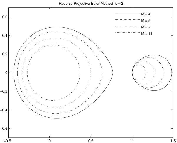
Figure 1: Stability Regions for Reverse Projective Methods.

3 Stationary Methods

In the above we have taken $M>k+1$ so that the net progress is negative in time. If we choose $M=k+1$ the total step length of the reverse projective integration method will be zero; we will call this a stationary projective method. It has the curious stability region shown in Figure 2. It is stable along a section of the real axis that includes $\rho=1$ (which is $h\lambda=0$). The boundary crosses itself at $\rho=1$. The intersection is at right angles because in the neighborhood of $\rho=1$ simple algebra shows that $\sigma$ is given by

$$\sigma=1-k(k+1)/2(\rho-1)^{2}-k^{2}(k-1)/2(\rho-1)^{3}$$ (1)

so the stability in the neighborhood of $\rho=1$ is equivalent to requiring that

$${\rm Real}((\rho-1)^{2})\geq 0$$

which happens when ${\rm Arg}(\rho)\in[-\pi/4,\pi/4]$ or $[3\pi/4,5\pi/4]$. The form of eq. (1) arises because the first-order accuracy of the method for a net step size of length zero means that

$$\sigma(0\lambda)=1+0\lambda+{\rm O}(h\lambda)^{2}=1+{\rm O}(\rho-1)^{2}$$

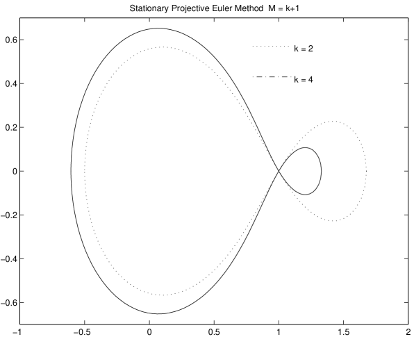
Figure 2: Stability Regions for Stationary Projective Methods.

It is possible that this procedure will be of value in the context of finding consistent initial conditions for differential algebraic equations (see [1]). If the algebraic components of a DAE were converted to stiff components (as has been advocated by some), the initialization problem is to find an initial condition that is “on the slow manifold” (i.e., the solution manifold of the original DAE.)

4 Comments

The procedure we just outlined will converge to saddle-type points whose linearization is characterized by a gap between strong stable modes and weak unstable ones. An existing forward simulation code will not in general converge to such points (the numerical trajectories will move away forward in time, and “explode away” backward in time). We can therefore think of our procedure as a computational superstructure that transforms a forward simulation code into a contraction mapping capable of converging to such saddle unstable points. The zero-net backward movement process described at the end can be related to consistent initialization algorithms for differential-algebraic equations.

Beyond the computation of saddle-type fixed points, however, if the forward in time dynamics possess such a separation of time scales globally, and an attracting, forward-invariant, low-dimensional slow manifold exists, the procedure becomes an “on manifold” reverse time integration scheme. That is, the regularizing action of the forward integration allows us to follow the on-manifold well-behaved trajectories backward in time. This may then provide a meaningful -and very simple to implement- way of regularizing the reverse, “on the slow manifold”, dynamics of stiff sets of ODEs and even discretizations of disspative PDEs. For example, in contexts where a low-dimensional inertial manifold exists for a dissipative PDE [4], our superstructure enables a direct simulation of an accurate discretization of the PDE to follow backward trajectories on the inertial manifold without ever having to explicitly derive an inertial form (or approximate inertial form).

In the spirit of the last observation, it is interesting to consider the implications of such a process for a meaningful reverse integration of systems described by microscopic/stochastic simulators. In many practically relevant cases, the coarse-grained behavior of such simulators can be described by the evolution in time of a few “master” moments of microscopically evolving distributions. The remaining, higher moments, become quickly slaved by forward simulation to the slow, master moments. We have recently proposed coarse projective integration schemes that use short bursts of appropriately initialized microscopic/stochastic simulation to estimate the time-derivative of the unavailable coarse equations for the master modes, and “project” these modes forward in time [5, 6, 7] If the coarse projection is performed backward in time, the procedure will allow us to follow the regularized reverse time behavior of the coarse variables. This is done using the microscopic/stochastic forward-in-time simulator directly, circumventing the necessity of deriving an explicit macroscopic closure. It becomes therefore possible to use a forward-in-time molecular dynamics simulator to extract regularized reverse-time information of coarse system variables. We have already demonstrated the feasibility of this technique in the case of coarse molecular dynamics simulations of a dipeptide folding kinetics in water [7]. Coarse reverse integration allows us to use microscopic simulators to quickly escape free-energy minima, to converge on certain transition states (saddles on the free-energy surface) and, more generally, may enhance our ability to explore the structure of free energy surfaces.

In summary, the technique holds promise towards (a) the computation of unstable, saddle-type fixed points using existing simulators; (b) the regularized, “on manifold” backward-in-time integration of certain dissipative PDEs possessing low-dimensional, exponentially attracting slow manifolds; and (c) the use of microscopic/stochastic simulators to track coarse-grained behavior backward in time, enhancing the ability to escape free energy minima and to locate saddle-type coarse-grained “transition states”.

Acknolwedgements. This work was partially supported by AFOSR (Dynamics and Control, Dr. B. King) and an NSF ITR grant. Discussions with Profs. P. G. Kevrekidis (UMass), Ju Li (OSU) and Dr. G. Hummer (NIH) are gratefully acknowledged.

References

- [1] Brown P. N., Hindmarsh A. C. and Petzold L. R. (1998). Consistent initial condition calculation for differential-algebraic systems, SIAM J. Sci. Comput., 19, 1495
- [2] Gear, C. W. and Kevrekidis, I. G, Projective Methods for Stiff Differential Equations: problems with gaps in their eigenvalue spectrum, NEC Research Institute Report 2001-029, in press, SIAM J. Sci. Comp.
- [3] Gear, C. W. and Kevrekidis, I. G, Telescopic Projective Methods for Stiff Differential Equations, NEC Research Institute Report 2001-122, in press, J. Comp. Phys.
- [4] Temam, R. (1988) Infinite Dimensional Dynamical Systems in Mechanics and Physics Springer Verlag, NY.
- [5] Gear, C. W., Kevrekidis, I. G. and Theodoropoulos, K. (2002) Coarse Integration/Bifurcation Analysis via Microscopic Simulators: micro-Galerkin methods, Comp. Chem. Engng. 26 pp.941-963
- [6] Siettos, C. I., Graham, M. D. and Kevrekidis, I. G. Coarse Brownian Dynamics Computations for Nematic Liquid Crystals” submitted to J. Chem. Phys.; can be obtained as cond-mat/0211455 at arXiv.org.
- [7] Hummer, G. and Kevrekidis, I. G. Coarse molecular dynamics of a peptide fragment: free energy, kinetics and long time dynamics computations”, submitted to J. Chem. Phys., Can be obtained as physics/0212108 at arXiv.org.