Wavefunction statistics in open chaotic billiards

Abstract

We study the statistical properties of wavefunctions in a chaotic billiard that is opened up to the outside world. Upon increasing the openings, the billiard wavefunctions cross over from real to complex. Each wavefunction is characterized by a phase rigidity, which is itself a fluctuating quantity. We calculate the probability distribution of the phase rigidity and discuss how phase rigidity fluctuations cause long-range correlations of intensity and current density. We also find that phase rigidities for wavefunctions with different incoming wave boundary conditions are statistically correlated.

Microwave cavities have been used as a quantitative experimental testing ground for theories of quantum chaos Stöckmann (1999). In quasi two-dimensional cavities, the component of the electric field perpendicular to the surface of the cavity satisfies a scalar Helmholtz equation that is formally equivalent to the Schrödinger equation. Complex field patterns, which model the wavefunction of an electron in a magnetic field, can be obtained making judicious use of magneto-optical effects So et al. (1995); Stoffregen et al. (1995). Alternatively, complex “wavefunctions” can be observed as travelling waves in open microwave cavities Pnini and Shapiro (1996); Barth and Stöckmann (2002). Measured distributions of real and complex wavefunctions in microwave cavities with chaotic ray dynamics, where, traditionally, “complex” means that time-reversal symmetry is fully broken and the phase of the wavefunction has no long-range correlations, agree with a theoretical description in terms of a random superposition of plane waves Berry (1977), as well as with random matrix theory Guhr et al. (1998) and supersymmetric field theories Efetov (1997).

Recently, it has become possible to study the full real-to-complex crossover using microwave techniques Barth and Stöckmann (2002); Chung et al. (2000). The crossover regime is qualitatively different from the “pure” cases of real or fully complex wavefunctions. Unlike in the pure cases, the statistical distribution of wavefunctions in the crossover regime depends on the choice of the ensemble: whether variations are taken with respect to the coordinate ${\bf r}$, the frequency $\omega$, or both. Whereas the theoretical work has been roughly equally divided between the two approaches, experiments usually need the additional average over frequency to obtain sufficient statistics So et al. (1995); Stoffregen et al. (1995); Wu et al. (1998); Chung et al. (2000) (see, however, Ref. Barth and Stöckmann, 2002 for an exception).

In general, a complex wavefunction may be written as

$$\psi({\bf r})=e^{i\phi}(\psi_{\rm r}({\bf r})+i\psi_{\rm i}({\bf r})),$$ (1)

where $\psi_{\rm r}$ and $\psi_{\rm i}$ are orthogonal but need not have the same normalization French et al. (1988). The ratio of $\psi_{\rm r}$ and $\psi_{\rm i}$ is parameterized in terms of the normalized scalar product of $\psi$ and its time-reversed,

$$\rho = \frac{\int d{\bf r}\,\psi({\bf r})^{2}}{\int d{\bf r}\,|\psi({\bf r})|^{2}}=e^{2i\phi}\frac{\int d{\bf r}\,|\psi_{\rm r}({\bf r})|^{2}-|\psi_{\rm i}({\bf r})|^{2}}{\int d{\bf r}\,|\psi_{\rm r}({\bf r})|^{2}+|\psi_{\rm i}({\bf r})|^{2}}.$$ (2)

The square modulus $|\rho|^{2}$ is known as the “phase rigidity” of the wavefunction $\psi$ van Langen et al. (1997). Real wavefunctions have $\rho=1$, whereas $\rho=0$ if $\psi$ is fully complex, i.e., $\psi_{\rm r}$ and $\psi_{\rm i}$ have the same magnitude. If the average is taken over the coordinate ${\bf r}$ only, whereas the frequency $\omega$ of the wavefunction is kept fixed, the wavefunction distribution follows by describing $\psi_{\rm r}$ and $\psi_{\rm i}$ as random superpositions of standing waves Źyczkowski and Lenz (1991); Kanzieper and Freilikher (1996); Pnini and Shapiro (1996). The resulting wavefunction distribution depends parametrically on the phase rigidity $|\rho|^{2}$. Using a microwave billiard with a movable antenna, Barth and Stöckmann have measured such a “single-wavefunction distribution” and found good agreement with the theory, obtaining $\rho$ from an independent measurement Barth and Stöckmann (2002). It is the fact that $\rho$ is different for each wavefunction that leads to the different results for averages over ${\bf r}$ only and over both ${\bf r}$ and $\omega$. A calculation of averages with respect to frequency requires a theory of the probability distribution of $\rho$. Such a full wavefunction distribution, which needs theoretical input beyond the ansatz that each wavefunction $\psi$ is a random superposition of plane waves, was first calculated by Sommers and Iida for the Pandey-Mehta Hamiltonian from random-matrix theory Sommers and Iida (1994) and by Fal’ko and Efetov Fal’ko and Efetov (1994, 1996) for a disordered quantum dot in a uniform magnetic field.

Fluctuations of the phase rigidity $|\rho|^{2}$ have been identified as the root cause for several striking phenomena in the crossover regime, such as long-range intensity correlations Fal’ko and Efetov (1996) and a non-Gaussian distribution of level velocities van Langen et al. (1997). Further, the existence of correlations between phase rigidities of different wavefunctions causes long-range correlations between wavefunctions at different frequencies Adam et al. (2002). The experimental verification of these effects addresses aspects of random wavefunctions that have not previously been tested. The relative magnitude of the phase rigidity fluctuations is numerically small, leading to long-range wavefunction correlations of order of 10 percent or less Fal’ko and Efetov (1996); Adam et al. (2002). This could explain why intensity distributions measured by Chung et al. could not distinguish between theories with and without phase rigidity fluctuations Chung et al. (2000).

In this letter, we consider wavefunctions in a billiard that is opened up to the outside world and calculate the probability distribution of phase rigidities for this case. Although time-reversal symmetry is not broken on the level of the wave equation itself, it is broken by the fact that one looks at a scattering state with incoming flux in one waveguide only Pnini and Shapiro (1996). As we show here, random wavefunctions in open cavities also have a fluctuating phase rigidity, and, hence, exhibit the same variety of phenomena as those in cavities with broken time-reversal symmetry, while they are much easier to generate in microwave experiments Barth and Stöckmann (2002). An additional advantage of the open-billiard geometry is the absence of fit parameters: The only parameter entering the wave-function distribution is the total number $N$ of propagating modes in the waveguides between the billiard and the outside world, which can be measured independently.

Following previous works on this subject, we consider the parameter regime in which the frequency average is taken over a window $\Delta\omega\ll c/L\ll\omega$, where $c$ is the velocity of wave propagation and $L$ the size of the billiard, and in which the openings occupy only a small fraction of the billiard’s boundary. It is only in this regime that wavefunctions have a universal distribution and a description in terms of a random superposition of plane waves is appropriate. We limit ourselves to (quasi) two-dimensional billiards, in which the electric field perpendicular to the billiard plane is identified with the wavefunction $\psi$ and the Poynting vector with the current density ${\bf j}\propto\mbox{Im}\,\psi^{*}{\bf\nabla}\psi$ Šeba et al. (1999). A calculation of wavefunctions inside an open billiard is complementary to a transport study, for which one is primarily intersted in the relation between amplitudes of ingoing and outgoing waves in the waveguides attached to the billiard, not in the wavefunction inside the cavity. Single-wavefunction statistics in open billiards in the universal regime was first considered by Pnini and Shapiro Pnini and Shapiro (1996) and subsequently by Ishio et al. Ishio et al. (2001); Saichev et al. (2002). Experimentally, wavefunctions in open billiards were investigated by Barth and Stöckmann Barth and Stöckmann (2002).

The key to the calculation of $P(\rho)$ in an open cavity is a relation between the scalar products of the in-cavity parts of scattering states $\psi_{\mu}$ and $\psi_{\nu}$ and the Wigner-Smith time-delay matrix $Q$ Smith (1960),

$$\int_{\rm cavity}d{\bf r}\psi_{\mu}({\bf r})\psi_{\nu}^{*}({\bf r})=Q_{\mu\nu},\ \$$ (3)

where the scattering states have been normalized to unit incoming flux. Here the index $\mu=1,\ldots,N$ labels the waveguide and the transverse mode from which the field is injected into the cavity. The time-delay matrix $Q=-iS^{\dagger}{\partial S}/{\partial\omega}$ is the derivative of the scattering matrix $S$. In order to calculate the scalar product $\rho_{\mu\mu}$ of the scattering state $\psi_{\mu}$ and its time-reversed $\psi_{\mu}^{*}$, we perform a unitary transformation $U$ that diagonalizes the Wigner-Smith time-delay matrix $Q$ and rotates the scattering matrix $S$ to the unit matrix Brouwer et al. (1997),

$$S=U^{\rm T}U,\ \ Q=U^{\dagger}\mbox{diag}\,(\tau_{1},\ldots,\tau_{N})U.$$ (4)

The positive numbers $\tau_{i}$, $i=1,\ldots,N$, are the “proper delay times”, the eigenvalues of the Wigner-Smith time-delay matrix. Note that the incoming modes are transformed according to the unitary transformation $U$, while the outgoing modes transform according to $U^{*}$, as required by time-reversal symmetry. In the transformed basis, all scattering states are standing waves and, hence, have $\rho_{jj}=1$. Transforming back to the original basis, we find

$$\rho_{\mu\mu}=\frac{\sum_{j=1}^{N}U_{j\mu}^{2}\tau_{j}}{\sum_{j=1}^{N}|U_{j\mu}|^{2}\tau_{j}}.$$ (5)

The joint distribution of the scattering matrix $S$ and the Wigner-Smith time-delay matrix $Q$ of a chaotic billiard is known from random-matrix theory Beenakker (1997): The distribution of the proper time delays $\tau_{i}$ is Brouwer et al. (1997)

$$P(\tau_{1},\ldots,\tau_{N}) = \prod_{j=1}^{N}\theta(\tau_{j})\tau_{j}^{-3N/2-1}e^{-N\tau_{\rm av}/2\tau_{j}}$$ (6)

$$\mbox{}\times\prod_{i<j}|\tau_{i}-\tau_{j}|,$$

where $\tau_{\rm av}$ is the average delay time and $\theta(x)=1$ for $x>0$ and $0$ otherwise, whereas the unitary matrix $U$ is uniformly distributed in the group of unitary $N\times N$ matrices. A numerical evaluation of the probability distribution of the phase rigidity $|\rho|^{2}$ is shown in Fig. 1 for several values of $N$. For the case $N=2$ of two single-mode waveguides, the probability distribution $P(\rho)$ can be found in closed form,

$$P(\rho) = \frac{6+2(1-|\rho|^{2})^{-1/2}}{3\pi(1+(1-|\rho|^{2})^{1/2})^{3}},\ \ 0\leq|\rho|<1.$$ (7)

For a billiard coupled to the outside world via $N\gg 1$ channels $P(\rho)$ becomes Gaussian,

$$P(\rho)=\frac{N}{4\pi}e^{-N|\rho|^{2}/4}.$$ (8)

This is the same functional form as the phase-rigidity distribution for a quantum dot in a large uniform magnetic field Fal’ko and Efetov (1994, 1996); van Langen et al. (1997).

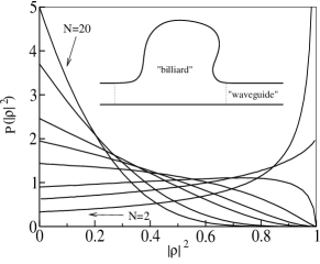
Figure 1: Probability distribution of the phase rigidity $|\rho|^{2}$ for a wavefunction in an open chaotic billiard, for different numbers of propagating modes connecting the billiard to the outside world. From bottom to top at the left end of the figure, curves correspond to $N=2$, $3$, $4$, $6$, $8$, $10$, $15$, and $20$. Inset: schematic drawing of billiard and waveguides.

Following Refs. Źyczkowski and Lenz, 1991; Pnini and Shapiro, 1996; Saichev et al., 2002, the joint distributions of intensities and current densities away from the boundary of the cavity for one wavefunction $\psi_{\mu}$ can then be calculated from Berry’s ansatz that $\psi_{\mu}$ can be written as a random superposition of plane waves Berry (1977),

$$\psi_{\mu}({\bf r})=\sum_{{\bf k}}a_{\mu}({\bf k})e^{i{\bf k}\cdot{\bf r}}.$$ (9)

In Eq. (9), all wavevectors ${\bf k}$ have the same modulus, while the amplitudes $a_{\mu}({\bf k})$ are random complex numbers. For a closed cavity, amplitudes of time-reversed plane waves are related, $a_{\mu}({\bf k})=e^{2i\phi}a_{\mu}(-{\bf k})^{*}$, where $\phi$ does not depend on ${\bf k}$. For an open cavity, no such strict relation exists, although some degree of correlation between $a_{\mu}({\bf k})$ and $a_{\mu}(-{\bf k})$ persists in order to ensure the correct value of the scalar product of $\psi_{\mu}$ and $\psi^{*}_{\mu}$, cf. Eq. (2) Saichev et al. (2002),

$$\rho_{\mu\mu}=\frac{\sum_{{\bf k}}a_{\mu}({\bf k})a_{\nu}(-{\bf k})}{\sum_{{\bf k}}|a_{\mu}({\bf k})|^{2}}.$$ (10)

Taking the amplitudes corresponding to wavevectors pointing in different directions from identical and independent distributions, we see that Eq. (10) implies a relation between the second moments of the amplitude distribution,

$$\langle a_{\mu}({\bf k})a_{\mu}(-{\bf k})\rangle = \rho_{\mu\mu}\langle|a_{\mu}({\bf k})|^{2}\rangle.$$ (11)

This, together with the normalization condition $\sum_{{\bf k}}\langle|a({\bf k})|^{2}\rangle=1/A$, where $A$ is the area of the billiard, and the central limit theorem, provides sufficient information to determine the full distribution of the wavefunction $\psi$.

As an example, we consider the joint distribution of the normalized intensity $I({\bf r})=|\psi({\bf r})|^{2}A$ and the magnitude of the normalized current density $J=|{\bf j}({\bf r}^{\prime})|$, ${\bf j}=(A/k)\mbox{Im}\,\psi^{*}{\bf\nabla}\psi$ at the positions ${\bf r}$ and ${\bf r}^{\prime}$ where $k=\omega/c$. The single-wavefunction distribution factorizes into separate probability distributions for $I$ and $J$ that each depend parametrically on the phase rigidity $|\rho|^{2}$ Źyczkowski and Lenz (1991); Saichev et al. (2002),

$$P_{\rho}[I({\bf r}),J({\bf r}^{\prime})] = \frac{8J}{(1-|\rho|^{2})^{3/2}}\,K_{0}\left(\frac{2J\sqrt{2}}{\sqrt{1-|\rho|^{2}}}\right)$$

$$\mbox{}\times I_{0}\left(\frac{I|\rho|}{1-|\rho|^{2}}\right)\exp\left(-\frac{I}{1-|\rho|^{2}}\right),$$

where $I_{0}$ and $K_{0}$ are Bessel functions. When both position and frequency are varied to obtain the ensemble average, a further average over $\rho$ is required,

$$P(I({\bf r}),J({\bf r}^{\prime}))=\int d\rho P(\rho)P_{\rho}(I({\bf r}),J({\bf r}^{\prime})).$$ (13)

After such average, $P(I,J)$ no longer factorizes. The degree of correlation is measured through the correlator

$$\langle I({\bf r})^{2}J({\bf r}^{\prime})^{2}\rangle_{c} = -\frac{1}{2}\mbox{var}\,|\rho|^{2},$$ (14)

where $\langle AB\rangle_{c}=\langle AB\rangle-\langle A\rangle\langle B\rangle$ denotes the connected average. (Since normalization implies that $\langle I({\bf r})\rangle=1$ for each wavefunction, correlators involving the first power of $I$ factorize.) For a billiard with two single-mode waveguides, $\mbox{var}\,|\rho|^{2}=8(148\ln 2-128(\ln 2)^{2}-41)/9\approx 0.078$, cf. Eq. (7). Similarly, we find for the correlator of intensities

$$\langle I({\bf r})^{2}I({\bf r}^{\prime})^{2}\rangle_{c} = \mbox{var}\,|\rho|^{2},$$ (15)

plus additional terms that describe short-range correlations.

Thus far we have studied the distribution of a single scattering state in an open billiard. However, for a billiard that is coupled to the outside world via, in total, $N$ propagating modes, there are $N$ orthogonal scattering states at each frequency. In the remainder of this letter we address the question of possible correlations between these scattering states.

This question can be studied using the framework of Ref. Adam et al., 2002, which generalizes the above considerations to the problem of correlations between wavefunctions. Again, the starting point is Berry’s ansatz (9), with a different set of amplitudes $a_{\mu}({\bf k})$ for each scattering state $\psi_{\mu}$, $\mu=1,\ldots,N$. We continue to take amplitudes $a_{\mu}({\bf k})$ from identical and independent distributions for different directions of ${\bf k}$, whereas we allow for correlations between amplitudes of time-reversed waves and between amplitudes of different scattering states. Such correlations are necessary, because the in-cavity parts of different scattering states and their time-reversed states are not orthogonal, see, e.g., Eq. (3). Hence, the second moments of the amplitudes $a_{\mu}({\bf k})$ should be chosen such that

$$n_{\mu\nu} \equiv \frac{\sum_{{\bf k}}a_{\mu}({\bf k})a_{\nu}({\bf k})^{*}}{(\sum_{{\bf k}}|a_{\mu}({\bf k})|^{2})^{1/2}(\sum_{{\bf k}}|a_{\nu}({\bf k})|^{2})^{1/2}},$$ (16)

$$= \frac{\int d{\bf r}\,\psi_{\mu}({\bf r})^{*}\psi_{\nu}({\bf r})}{(\int d{\bf r}\,|\psi_{\mu}({\bf r})|^{2}\int d{\bf r}^{\prime}\,|\psi_{\nu}({\bf r}^{\prime})|^{2})^{1/2}},$$

$$\rho_{\mu\nu} \equiv \frac{\sum_{{\bf k}}a_{\mu}({\bf k})a_{\nu}(-{\bf k})}{(\sum_{{\bf k}}|a_{\mu}({\bf k})|^{2})^{1/2}(\sum_{{\bf k}}|a_{\nu}({\bf k})|^{2})^{1/2}}$$ (17)

$$= \frac{\int d{\bf r}\,\psi_{\mu}({\bf r})\psi_{\nu}({\bf r})}{(\int d{\bf r}\,|\psi_{\mu}({\bf r})|^{2}\int d{\bf r}^{\prime}\,|\psi_{\nu}({\bf r}^{\prime})|^{2})^{1/2}},$$

where, as before, the integrals are taken over the billiard only and we have chosen the normalization such that $n_{\mu\mu}=1$. Equations (16) and (17) then impose the following relations for second moments of the amplitude distributions:

$$\langle a_{\mu}({\bf k})a_{\nu}({\bf k})^{*}\rangle = n_{\mu\nu}\langle|a_{\mu}({\bf k})|^{2}\rangle,$$ (18)

$$\langle a_{\mu}({\bf k})a_{\nu}(-{\bf k})\rangle = \rho_{\mu\nu}\langle|a_{\mu}({\bf k})|^{2}\rangle.$$ (19)

Repeating the same arguments as those leading to Eq. (5), we find that $n_{\mu\nu}$ and $\rho_{\mu\nu}$ can be expressed in terms of eigenvectors and eigenvalues of the time-delay matrix,

$$n_{\mu\nu} = \frac{\sum_{j}U_{j\mu}^{*}U_{j\nu}\tau_{j}}{(\sum_{j}|U_{j\mu}|^{2}\tau_{j}\sum_{i}|U_{i\nu}|^{2}\tau_{i})^{1/2}},$$

$$\rho_{\mu\nu} = \frac{\sum_{j}U_{j\mu}U_{j\nu}\tau_{j}}{(\sum_{j}|U_{j\mu}|^{2}\tau_{j}\sum_{i}|U_{i\nu}|^{2}\tau_{i})^{1/2}}.$$ (20)

The full distribution of the complex numbers $n_{\mu\nu}$ and $\rho_{\mu\nu}$ then follow from the known distributions of the $N\times N$ unitary matrix $U$ and the proper time delays $\tau_{j}$, $j=1,\ldots,N$. A simple expression is obtained in the limit $N\gg 1$, when $n_{\mu\nu}$ and $\rho_{\mu\nu}$ acquire a Gaussian distribution, with zero mean and with variance given by

$$\langle n_{\mu\nu}n_{\sigma\tau}\rangle=\frac{1}{N}\delta_{\mu\tau}\delta_{\nu\sigma}\ \ \mbox{if $\mu\neq\nu$},$$

$$\langle\rho_{\mu\nu}\rho_{\tau\sigma}^{*}\rangle=\frac{2}{N}(\delta_{\mu\tau}\delta_{\nu\sigma}+\delta_{\mu\sigma}\delta_{\nu\tau}),$$

$$\langle n_{\mu\nu}\rho_{\sigma\tau}\rangle=\langle\rho_{\mu\nu}\rho_{\tau\sigma}\rangle=0.$$ (21)

Short range correlations between different scattering modes arise from the fact that $\rho_{\mu\nu}$ and $n_{\mu\nu}$ are nonzero for $\mu\neq\nu$. These correlations exist both if statistics is taken as a function of position only and if the ensemble also involves a frequency average. For example, for the second moment of the intensity and current density distributions, we find from Eq. (9)

$$\langle I_{\mu}({\bf r})I_{\nu}({\bf r}^{\prime})\rangle_{c} = (|n_{\mu\nu}|^{2}+|\rho_{\mu\nu}|^{2})J_{0}(k|{\bf r}-{\bf r}^{\prime}|),$$ (22)

$$\langle j_{\mu,\alpha}({\bf r})j_{\nu,\beta}({\bf r}^{\prime})\rangle = \frac{1}{4}\delta_{\alpha\beta}(|n_{\mu\nu}|^{2}+|\rho_{\mu\nu}|^{2})J_{0}(k|{\bf r}-{\bf r}^{\prime}|),$$

with $\alpha,\beta=x,y$. For the case $N=2$ of a billiard with two single-mode waveguides one has $\langle|\rho_{12}|^{2}\rangle=(64\ln 2-37)/15\approx 0.49$ and $\langle|n_{12}|^{2}\rangle=(26-32\ln 2)/15\approx 0.25$. Long-range correlations arise from the fluctuations of the “scalar products” $n_{\mu\nu}$ and $\rho_{\mu\nu}$ and exist only if the ensemble involves a frequency average. The lowest moment with long-range correlations is

$$\langle I_{\mu}({\bf r})^{2}I_{\nu}({\bf r}^{\prime})^{2}\rangle_{c} = -2\langle I_{\mu}({\bf r})^{2}J_{\nu}({\bf r}^{\prime})^{2}\rangle_{c}$$

$$= \langle|\rho_{\mu\mu}|^{2}|\rho_{\nu\nu}|^{2}\rangle-\langle|\rho_{\mu\mu}|^{2}\rangle\langle|\rho_{\nu\nu}|^{2}\rangle.$$

For $N=2$ one has $\langle|\rho_{11}|^{2}|\rho_{22}|^{2}\rangle-\langle|\rho_{11}|^{2}\rangle\langle|\rho_{22}|^{2}\rangle=8(5792\,\ln 2-4480(\ln 2)^{2}-1861)/315\approx 0.032$.

In conclusion, we have calculated the wavefunction distribution for wavefunctions in an open chaotic billiard for the case that the ensemble average involves both an average over frequency and position. Fluctuations and correlations of the phase rigidities lead to long range correlations between intensities and current densities. Our results are relevant for a fit-parameter free measurement of the real-to-complex wavefunction crossover.