Chapter 0 Nonlinear Vibration in Gear Systems G. Litak and M.I. Friswell

Grzegorz Litak¹ and Michael I. Friswell²

Gear box dynamics is characterised by a periodically changing stiffness and a backlash which can lead to a loss of the contact between the teeth. Due to backlash, the gear system has piecewise linear stiffness characteristics and, in consequence, can vibrate regularly or chaoticaly depending on the system parameters and the initial conditions. We examine the possibility of a nonfeedback system control by introducing a weak resonant excitation term and through adding an additional degree of freedom to account for shaft flexibility on one side of the gearbox. We shall show that by correctly choosing the coupling values the system vibrations may be controlled.

1 Introduction

Gear box dynamics is based on a periodically changing meshing stiffness complemented by a nonlinear effect of backlash between the teeth. Recently, their regular and chaotic vibrations have been predicted theoretically and examined experimentally [2, 3, 4, 5, 6, 7, 8]. The theoretical description of this phenomenon has been based mainly on single degree of freedom models [2, 3, 4, 5, 6, 7, 9] or multi degree models neglecting backlash [10, 11]. This paper examines the possibility of taming chaotic vibrations and reducing the amplitude by nonfeedback control methods. Firstly, we will introduce a weak resonant excitation through an additional small external excitation term (torque) with a different phase [12, 13]. Secondly, we will examine the effect of an additional degree of freedom to account for shaft flexibility on one side of the gearbox [8]. This may also be regarded as a single mode approximation to the torsional system dynamics, or alternatively as a simple model for a vibration neutraliser or absorber installed in one of the gears.

2 One Stage Gear Model

We start our analysis with modelling the relative vibrations of a single stage transmission gear [7]. Figure 1 shows a schematic picture of the physical system. The gear wheels are shown with moments of inertia $I_{1}$ and $I_{2}$ and are coupled by the stiffness and damping of the teeth mesh, represented by $k_{Z}$ and $c_{Z}$.

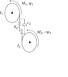
Figure 1: The physical model of a one stage transmission gear system.

The equations of motion of the system may be written in terms of the two degrees of freedom, $\psi_{1}$, $\psi_{2}$ that represent the rotational angles of the gear wheels. These angles are those that remain after the steady rotation of the system is removed [7]. Thus, if the backlash is initially neglected, we have

$$I_{1}\ddot{\psi}_{1}+\left[k_{Z}(r_{1}\psi_{1}-r_{2}\psi_{2})+c_{Z}(r_{1}\dot{\psi}_{1}-r_{2}\dot{\psi}_{2})\right]r_{1} = M_{1},$$

$$I_{2}\ddot{\psi}_{2}-\left[k_{Z}(r_{1}\psi_{1}-r_{2}\psi_{2})+c_{Z}(r_{1}\dot{\psi}_{1}-r_{2}\dot{\psi}_{2})\right]r_{2} = -M_{2},$$ (1)

where $r_{1}$ and $r_{2}$ are the radii of the gear wheels and the overdot represents differentiation with respect to time $t$.

Figure 2: The meshing stiffness $k(\tau)$.

Figure 3: The amplitude of vibration (a) and the maximal Lyapunov exponent $\lambda_{1}$ (b) versus frequency $\omega$ obtained by simulation. The initial conditions were assumed to be $x_{0}=-2.0$ and $v_{0}=\dot{x}_{0}=-0.5$ for small $\omega$ ($\omega_{0}=0.1$) and for each new $\omega$ ($\omega_{i+1}$) calculations were performed for $400$ excitation cycles. Each time new initial conditions $(x_{0},v_{0})$ were chosen as the last pair of values of $(x,v)$ for previous $\omega_{i}$ ($(x_{0},v_{0})|_{new}=(x,v)|_{old}$). Curves ’1’ and ’2’ correspond to cases with $D=0$ and $D=2$, respectively.

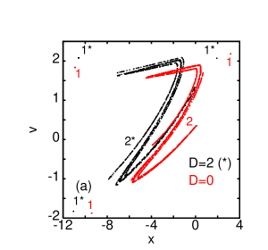
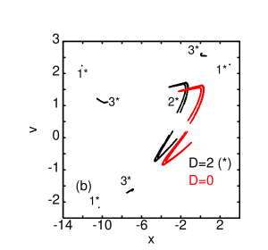
Figure 4: The Poincare maps calculated for ten randomly chosen initial conditions for $\omega=1.5$ (a) and $\omega=1.6$ the gray colour corresponds to simulations with respect to (Eq. 2) while the black one to (Eq. 6), respectively.

In fact, it is possible to reduce the above two equations to one using the new relative displacement coordinate $x=r_{1}\psi_{1}-r_{2}\psi_{2}$. That coordinate represents the relative displacement of the gear wheels at the teeth. The equation of motion for $x$ is obtained by subtracting $r_{2}/I_{2}$ times first equation from $r_{1}/I_{1}$ times the second one (Eqs. 1). Thus, in non-dimensional form, the equation of motion can be rewritten as

$$\frac{{\rm d}^{2}}{{\rm d}\tau^{2}}x+\frac{2\zeta}{\omega}\frac{{\rm d}}{{\rm d}\tau}x+\frac{k(\tau)g(x,\eta)}{\omega^{2}}=\frac{\bar{B}(\tau)}{\omega^{2}}=\frac{B_{0}+B_{1}cos(\tau+\Theta)}{\omega^{2}},$$ (2)

where the parameters are easily derived from Eqs. (1-2), as

$$\tau = \omega t,$$

$$2\zeta = c_{Z}\left[r_{1}^{2}/I_{1}+r_{2}^{2}/I_{2}\right],$$ (3)

$$\bar{B}(\tau) = r_{1}M_{1}/I_{1}+r_{2}M_{2}/I_{2}.$$

$\zeta$, $k(\tau)$, $g(x,\eta)$ and $\bar{B}(\tau)$ are defined as in reference [7]. Note that the backlash and time dependent meshing stiffness have been included by rewriting the meshing force as [7]

$$k_{Z}\left[r_{1}^{2}/I_{1}+r_{2}^{2}/I_{2}\right]x=k(\tau)g(x,\eta).$$ (4)

Equations (3) and (4) have assumed that the moments on the gear system are composed of a sinusoidal moment at frequency $\omega$ with a constant offset.

The meshing stiffness is periodic and the backlash is described by a piecewise linear function. Figure 2 shows a typical time dependent mesh stiffness variation $k(\tau)$ [7] and the backlash is modelled for a clearance $\eta$ as

$$g\left({x,\eta}\right)=\left\{{\begin{array}[]{*{20}c}x&&{x\geq 0}\\ 0&&{-\eta<x<0}\\ {x+\eta}&&{x\leq\eta}.\\ \end{array}}\right.$$ (5)

3 Vibrations of a Gear System in Presence of a Weak Resonance Term

Now we are going to examine the gear system described by Eqs. (1-5) subjected to to an additional external periodic excitation with a relatively small value $D$

$$\frac{{\rm d}^{2}}{{\rm d}\tau^{2}}x+\frac{2\zeta}{\omega}\frac{{\rm d}}{{\rm d}\tau}x+\frac{k(\tau)g(x,\eta)}{\omega^{2}}=\frac{B_{0}+B_{1}cos(\tau+\Theta)+Dcos(\tau+\Theta^{\prime})}{\omega^{2}},$$ (6)

where the phase angle $\Theta^{\prime}\neq\Theta$. Such inclusion has been discussed earlier in the literature as a suitable method of chaos control for Josephson junction circuits [12] and Froude pendulum motion [13]. In those papers the authors claimed that the resonant term, if used adequately, can tame or include chaotic motion. We have performed numerical simulations of Eqs. (2) and (6) to highlight the effect of the addition of resonant term $D$ on the basic equation of motion (Eq. 2). In particular we were interested in changes in vibration amplitude. The type of motion was analysed using Lyapunov exponents obtained by the algorithm of Wolf et al. [14]. System parameters have been used as in [7]: $\omega=1.5$, $B_{0}=1$, $B_{1}=4$, $\Theta=0$, $\zeta=0.08$, $\eta=10$ while the additional excitation term 6 was introduced as $D=2$, $\Theta^{\prime}=0.1$.

Figure 3a shows the calculated vibration amplitude of the relative motions of the gear wheels, $A$, defined as

$$A=\left|\frac{x_{max}-x_{min}}{2}\right|.$$ (7)

The maximal Lyapunov exponent $\lambda_{1}$ versus frequency $\omega$, obtained by simulation, is plotted in Fig. 3b. Note, the initial conditions were assumed to be $x_{0}=-2.0$ and $v_{0}=\dot{x}_{0}=-0.5$ for small starting $\omega$ ($\omega=0.1$) and for each new $\omega_{i+1}$ calculations were performed for $400$ excitation cycles with where new initial conditions were the last pair of values of $(x,v)$ for the previous frequency $\omega_{i}$. Curves marked by ’1’ correspond to solutions of Eq. 2 while those marked by ’2’ correspond to Eq. 6. One can easily note that the amplitude of the modified system is slightly larger but simultaneously the system behaves more regularly. In most of cases where the original system was in a chaotic state ($\lambda_{1}>1$ for the curve ’1’, Fig. 3b) it vibrates regularly in the presence resonant term ($\lambda_{1}<1$ for the curve ’2’ in Fig. 3b). Unfortunately the taming of the chaotic motion was accompanied by additional features visible in Fig. 3a. Clearly, the curve ’2’ describing the amplitude of motion shows a number of jumps, i.e. for $\omega\approx 1.36$ and 1.70. These jumps may be associated with transitions to other solutions (attractors) with changing $\omega$. This effect is typical for many nonlinear systems but it seems to be more transparent for $D\neq 0$. To explore further this effect we have also calculated Poincare maps for many initial conditions chosen randomly. The results for frequencies $\omega=1.5$ and 1.6 are shown in Fig. 4. In this figure, one can see that for $\omega=1.5$ attractors (in gray colour) for $D=0$ and (in black colour) for $D\neq 0$ are similar. Here, numbers ’1’ and ’2’ denote the regular and chaotic attractors, respectively. But if we move $\omega$ to a larger value ($\omega$= 1.6) the regular attractor for $D=0$ disappears. The attractor remains for $D\neq 0$, but interestingly another chaotic attractor emerges. For some other frequencies additional attractors also exist, which supports the proposed explanation of the jumping phenomenon.

4 Vibrations of a Gear System with a Flexible Shaft

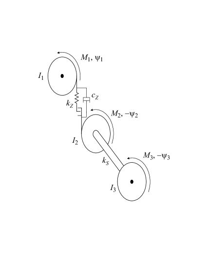
Figure 5: The physical model of the gear model with an additional degree of freedom introduced by a disk fixed by a flexible shaft to one of gear wheels.

Here we examine the effect of adding an additional degree of freedom to the gear system (Fig. 5) by using a flexible shaft on one side of the gearbox [8].

Now the equations of motion of the system may be written in terms of the three degrees of freedom, $\psi_{1}$, $\psi_{2}$ and $\psi_{3}$, related to the rotational angles of the gear wheels and disk, and have the following form

$$I_{1}\ddot{\psi}_{1} + \left[k_{Z}(r_{1}\psi_{1}-r_{2}\psi_{2})+c_{Z}(r_{1}\dot{\psi}_{1}-r_{2}\dot{\psi}_{2})\right]r_{1}=M_{1},$$

$$I_{2}\ddot{\psi}_{2} - \left[k_{Z}(r_{1}\psi_{1}-r_{2}\psi_{2})+c_{Z}(r_{1}\dot{\psi}_{1}-r_{2}\dot{\psi}_{2})\right]r_{2}-k_{S}(\psi_{3}-\psi_{2})=-M_{2},$$

$$I_{3}\ddot{\psi}_{3} + k_{S}(\psi_{3}-\psi_{2})=-M_{3}.$$ (8)

Figure 6: The amplitude of vibration (a) and the maximal Lyapunov exponent $\lambda_{1}$ (b) versus frequency $\omega$ obtained by simulations. The initial conditions were assumed to be $x_{10}=-2.0$, $v_{10}=\dot{x}_{10}=-0.5$ and $x_{20}=0$ $v_{20}=\dot{x}_{20}=0$ for small $\omega$ ($\omega=0.1$) and for each new $\omega_{i+1}$ calculations were performed for $400$ excitation cycles where the new initial conditions were the last pair of values of $(x_{1},v_{1},x_{2},v_{2})$ for the previous $\omega_{i}$. Curves ’1’,’2’,’3’ were obtained for $k_{S}=0$, 0.1 and 1.0, respectively. Four nonzero Lyapunov exponents $\lambda_{i}$ ($i=1,2,3,4$) versus frequency $\omega$ are shown for $k_{S}=0.1$ (c) and $k_{S}=1.0$ (d).

As in the previous case (Eqs. 1, 2) the above set of equations may be decoupled by using the new relative displacement coordinates $x_{1}=r_{1}\psi_{1}-r_{2}\psi_{2}$ and $x_{2}=r_{2}(\psi_{3}-\psi_{2})$. Thus we reduce the number of equations from three to two

$$\frac{{\rm d}^{2}}{{\rm d}\tau^{2}}x_{1} + \frac{2\zeta}{\omega}\frac{{\rm d}}{{\rm d}\tau}x_{1}+\frac{k(\tau)g(x_{1},\eta)}{\omega^{2}}+\frac{\beta_{1}k_{S}x_{2}}{\omega^{2}}$$ (9)

$$= \frac{B_{0}+B_{1}cos(\omega t+\Theta)}{\omega^{2}},$$

$$\frac{{\rm d}^{2}}{{\rm d}\tau^{2}}x_{2} + \frac{\beta_{2}k_{S}x_{2}}{\omega^{2}}+\frac{2\beta_{3}\zeta}{\omega}\frac{{\rm d}}{{\rm d}\tau}x_{1}+\frac{\beta_{3}k(\tau)g(x_{1},\eta)}{\omega^{2}}=0,$$

where most of parameters have already been defined in Eqs. 3 and 4. The rest of them are easily derived from Eqs. (8-9), as

$$\beta_{1} = 1/I_{2},$$

$$\beta_{2} = 1/I_{2}+1/I_{3},$$

$$\beta_{3} = (r_{2}^{2}/I_{2})/\left[r_{1}^{2}/I_{1}+r_{2}^{2}/I_{2}\right],$$ (10)

$$0 = r_{2}M_{2}/I_{2}-r_{2}M_{3}/I_{3}.$$

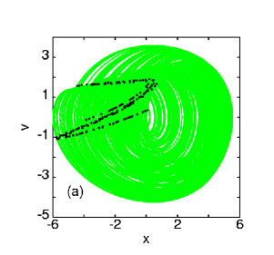
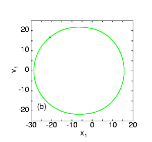
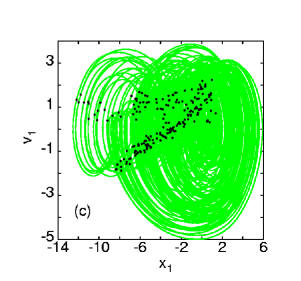
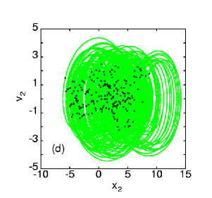
Figure 7: Phase portraits (gray lines) and Poincare maps (black points) for $\omega=1.5$ and $k_{S}=0$ (a), $k_{S}=1.0$ (b) and $k_{S}=0.1$ (c-d). The initial conditions: $x_{10}=-2.0$, $v_{10}=\dot{x}_{10}=-0.5$ and $x_{20}=0$ $v_{20}=\dot{x}_{20}=0$.

The simulation results of the above system (Eq. 9, Fig. 5) are presented in Fig. 6 and 7. First of all we have repeated the calculations of the amplitude and Lyapunov exponents. The results for the amplitude $A$ with various couplings ($k_{S}$) are summarized in Fig. 6a. Curves ’1’,’2’,’3’ correspond to for $k_{S}=0$, 0.1 and 1.0, respectively. One can see that a suitable change to $k_{S}$ may lead to the lowering of the amplitude. This effect is more efficient in the case of $k_{S}=1.0$. Comparing the corresponding values of the maximal Lyapunov exponents one can investigate the chaotic nature of the vibrations (Fig. 6b). Namely, the case $k_{S}=0.1$ (the curve ’2’) does not reduce the original chaoticity in region around $\omega\approx 1.0$ and $\omega\in[1.24,1.62]$ (the curve ’1’) while $k_{S}=1.0$ is large enough to tame the chaos in these regions as well as to make the vibration amplitude smaller.

It should be noted that for $k_{S}\neq 0$ there are four nonzero exponents to be examined. The positive value of the largest one $\lambda_{1}$, is presented in Fig. 6b. It detects frequency regions of chaotic vibrations. But it is also interesting to see what has happened to the other exponents, especially for our multidimensional system. They were also calculated and are plotted for comparison in Figs. 6c-d. For a small coupling stiffness, $k_{S}=0.1$, we have the surprising result that most of the chaotic regions are characterized by two positive exponents (Fig. 6c), which is a signal that the system is truly hyperchaotic [15, 16, 11]. In this case two initially close trajectories escape exponentially in two different directions. The results of calculations with larger $k_{S}$ ($k_{S}=1.0$) are different (Fig. 6), where regions of chaotic motion with only one positive Lyapunov exponent were found, which signals typical chaotic behaviour. To clarify this point we plot the phase portrait and Poincare maps for the chosen frequency $\omega=1.5$. Figure 7a shows the portrait plane and the Poincare map of chaotic attractor for $k_{S}=0$ while in Fig. 7b, for $k_{S}=1.0$, the corresponding attractor is regular, synchronized with the excitation frequency $\omega$. Figures 7c and d show the phase portrait and the Poincare map of the hyperchaotic attractor.

5 Conclusions

This paper has examined the effect of adding an additional small resonance excitation term or an additional degree of freedom to a simple model of gear vibration (Figs. 1 and 2). We have shown that the resonance term can successively reduce chaoticity in the dynamical system (Fig. 3b), although the vibration amplitude increases to a larger value than that for the basic system. We also noted several sudden jumps in the vibration amplitude value (Fig. 3a) which could destroy a real gearbox. The jumps are presumably caused by the creation of a larger number of attractors in the presence of the resonance term (Fig. 4). The extra degree of freedom (Fig. 5), which may represent a flexible shaft or a vibration neutraliser, also has a considerable effect on the dynamics. We noted that the suitable use of the coupling value, shaft stiffness $k_{S}$, can lead to regular attractors ($k_{S}=1.0$) and, simultaneously, to a reduction in the vibration amplitude (Fig. 6a-b). Interestingly we have found that for a small value of the coupling stiffness, $k_{S}=0.1$, two of the four Lyapunov exponents were positive, leading to hyperchaos phenomenon. The study of the hyperchaotic attactor will be reported in a separate article. Thus the coupling $k_{S}$ is a proper bifurcation parameter giving a wide range of system behaviour. The correct choice of this stiffness value can also be used to control the system vibrations.

References

- [1] [1]99
- [2] A. Kahraman and R. Singh, Non–linear dynamics of a spur gear pair, Journal of Sound and Vibration 142 (1990), 49–75.
- [3] K. Sato, S. Yammamoto, T. Kawakami, Bifurcation sets and chaotic states of a gear system subjected to harmonic excitation, Computational Mechanics 7 (1991), 171–182.
- [4] G.W. Blankenship and A. Kahraman, Steady state forced response of a mechanical oscillator with combined parametric excitation and clearance type non–linearity, Journal of Sound and Vibration 185 (1995), 743–765.
- [5] A. Kahraman and G.W. Blankenship, Experiments on nonlinear dynamic behavior of an oscillator with clearance and periodically time–varying parameters, ASME Journal of Applied Mechanics 64 (1997), 217–226.
- [6] A. Raghothama and S. Narayanan, Bifurcation and chaos in geared rotor bearing system by incremental harmonic balance method, Journal of Sound and Vibration 226 (1999), 469–492.
- [7] J. Warmiński, G. Litak, K. Szabelski, Dynamic phenomena in gear boxes, in M. Wiercogroch and B. De Kraker, editors. Applied nonlinear dynamics and chaos of mechanical systems with discontinuities, Series on Nonlinear Science Series A vol. 28, World Scientific, Singapore 2000, 177–205.
- [8] G. Litak and M.I. Friswell, Vibrations in gear systems, Chaos, Solitons & Fractals 16 (2003), 145–150.
- [9] K. Szabelski, G. Litak, J. Warmiński and G. Spuz–Szpos, Chaotic vibrations of the parametric system with baclash and non–linear elasticity, in Proc. of EUROMECH – 2nd European Nonlinear Oscillation Conference, vol. 1, Prague, September 1996, 431–435.
- [10] G. Schmidt, A. Tondl, Non-linear vibrations, Akademie-Verlag, Berlin 1986.
- [11] J. Warmiński, G. Litak and K. Szabelski, Synchronisation and chaos in a parametrically and self–excited system with two degrees of freedom, Nonlinear Dynamics 22 (2000), 135–153.
- [12] R. Chakon, F. Palmero and F. Balibrea, Taming chaos in a driven Josephson junction, International Journal of Bifurcation and Chaos 11 (2001), 1897–1909.
- [13] H. Cao, X. Chi and G. Chen, Suppresing or including chaos by weak resonant excitations in an externally-forced Froude pendulum, International Journal of Bifurcation and Chaos (2003), in press.
- [14] A. Wolf, J.B. Swift, H.L. Swinney and J.A. Vastano, Determining Lyapunov exponents from a time series, Physica D 16 (1988) 285–317.
- [15] T. Kapitaniak and L.O. Chua, Hyperchaotic attractors of undirectionally coupled Chua’s circuits, International Journal of Bifurcation and Chaos 4 (1994) 477–482.
- [16] J. Warmiński, G. Litak and K. Szabelski, Vibrations of a parametrically and self–excited system with two degrees of freedom, in Proc. of Second International Conference on Identification in Engineering Systems, Swansea, March 1999, (Eds. M.I. Friswell, J.M. Mottershead and A.W. Lees, University of Wales, Swansea 1999), 285–294.