Non-local Interaction Effects on Pattern Formation in Population Dynamics

Abstract

We consider a model for population dynamics such as for the evolution of bacterial colonies which is of the Fisher type but where the competitive interaction among individuals is non-local, and show that spatial structures with interesting features emerge. These features depend on the nature of the competitive interaction as well as on its range, specifically on the presence or absence of tails in, and the central curvature of, the influence function of the interaction.

Population dynamics covers a wide spectrum of fields. The formation of patterns in the evolution of bacterial colonies provides an example jaco ; waki ; lin ; nels ; thesis . Such studies, e.g., the growth of an initial nucleus of cells, are important within a clinical framework since the control of bacterial infections might be better performed if the dynamics of the growth of bacteria were understood at a basic level. The Streptococcus pyogenes or Group A streptococcus, that has been made famous in recent times by media reports of flesh-eating bacteria which claim the lives of up to 25% of its victims, provides one example. Processes related with cancer development provide another.

When dealing exclusively with the evolution of cell population and its spatio-temporal features, it is usual to focus attention on some processes such as reproduction, competition for resources, and diffusion, and to neglect others such as mutation. The Fisher equation is, therefore, a good starting for such studies. We show below new results concerning pattern formation that arise from a natural extension of the Fisher equation. This differential equation considers, besides the diffusion process with coefficient $D$, growth of the population at rate $a$ and a limiting process controlled by $b$, associated generally with competition or struggle for resources fish :

$$\frac{\partial u\left(x,t\right)}{\partial t}=D\frac{\partial^{2}u\left(x,t\right)}{\partial x^{2}}+au\left(x,t\right)-bu^{2}\left(x,t\right).$$ (1)

Our generalization consists in incorporating non-local effects in the competition terms:

$$\frac{\partial u\left(\vec{x},t\right)}{\partial t} = D\nabla^{2}u\left(\vec{x},t\right)+a\,u(\vec{x},t)$$

$$-b\,u(\vec{x},t)\int_{\Omega}u(\vec{y},t)f_{\sigma}(\vec{x},\vec{y}).$$

Here $f_{\sigma}(\vec{x},\vec{y})$ is a positive function or distribution which we call the influence function, characterized by a range $\sigma$, and normalized in the domain $\Omega$ under investigation. The physical origin of non-local aspects in the competition interaction is easy to understand. For instance, in the case of bacteria, the diffusion of nutrients and/or the release of toxic substances can cause non-locality in the interaction. While non-local competition has been mentioned earlier lee ; mog , we show below consequences of the non-local terms that have not been reported earlier, specifically, striking features of the dependence of the patterns on the nature as well as range of the influence function.

It is known that no patterns appear in the extreme local limit $f_{\sigma}(\vec{x},\vec{y})=\delta(\vec{x}-\vec{y})$ which reduces (Non-local Interaction Effects on Pattern Formation in Population Dynamics) to (1). No patterns appear in the extreme nonlocal limit either, where $f_{\sigma}(x)$ is a constant, as can be seen from an explicit analytical solution given by one of the present authors vmkpasi :

$$u(x,t)=\left[e^{-at}+\frac{b\overline{u}_{0}}{a}\left(1-e^{-at}\right)\right]^{-1}\int\Psi(x-y,t)u_{0}(y)dy,$$ (3)

where $\Psi\left(z,t\right)$ is the standard Gaussian propagator $(4\pi Dt)^{-1/2}exp(-z^{2}/4Dt)$ of the diffusion equation, and $\overline{u}_{0}$ is the integral over all space of the initial density $u_{0}(x)$. In the intermediate case, however, patterns do appear. The simplest forms for the influence function are a Gaussian and a square distribution. The latter is simply a normalized constant function within a range and vanishing outside. The former is given by

$$f_{\sigma}(x,y)=\alpha(x)\,\exp\left[-\frac{(x-y)^{2}}{2\sigma^{2}}\right]$$ (4)

in the 1-dimensional case. In the case of periodic boundary conditions with spatial period $L$, the normalization factor $\alpha(x)$ is a constant, $\frac{1}{\alpha}=\sqrt{\frac{\pi}{2}}\,\sigma\,\mbox{erf}\left(\frac{L}{\sqrt{2}\sigma}\right)$, whereas, for zero-flux boundary conditions, it is space-dependent:

$$\frac{1}{\alpha(x)}=\sqrt{\frac{\pi}{2}}\,\sigma\,\left[\mbox{erf}\left(\frac{x}{\sqrt{2}\sigma}\right)-\mbox{erf}\left(\frac{x-L}{\sqrt{2}\sigma}\right)\right].$$ (5)

Is is helpful to characterize the influence function by its width at the origin. For periodic boundary conditions, in which case $f_{\sigma}$ depends on the difference $z=x-y$, this width is given by $\Sigma=\left[-d^{2}(\mbox{ln}(f_{\sigma})/dz^{2})_{z=0}\right]^{-1/2}$, equals $\sigma$ for a Gaussian, and is infinite for the square function.

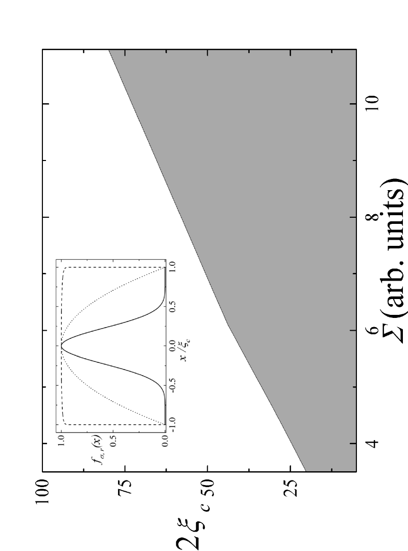
Our calculations show that, for the case of the square influence function (infinite $\Sigma$), patterns of nontrivial amplitude appear for all values of the cut-off interval of the square, the amplitude of the peaks being not uniform but presenting a periodic modulation. For a Gaussian influence function (finite $\Sigma$), the patterns exhibit a curious feature in the periodic boundary condition case. Two critical values of the width $\Sigma$ are seen separating trivial patterns with vanishing amplitude from nontrivial patterns with substantial amplitude foot . This is displayed in Figs. 1 and 2.

Figure 1: Dramatic difference in the amplitude of the steady state patterns with Gaussian influence function and periodic boundary conditions, for $\Sigma/L=$ a) $0.205$, b)$0.245$ and c)$12$. Here, $u(x)$ is plotted in units of $a/b$, and $x$ in units of $L$.

The critical width depends linearly on the domain size $L$ (with a slight deviation for small domains) making it possible to display our results with $\Sigma/L$ on the x-axis. The results displayed are for a system size $L$ of 100 sites with $D=1\times 10^{-3}$, $a=1$, $b=1$, in arbitrary but consistent units. A plot of the pattern amplitude $A_{0}$ (see Fig. 2) shows a striking transition around the value $2/9$ of the ratio $\Sigma/L$.

Figure 2: Dependence of the amplitude of the patterns on the ratio of the width of the influence function to the domain size. Inset, which depicts the small $\Sigma/L$ behavior on an expanded scale, shows an apparent transition around the value $2/9$ of $\Sigma/L$. The arrows mark the three patterns depicted in Fig. 1.

Is this sharp difference between square and Gaussian influence functions the result of the cut-off inherent in the former? In particular, could the sudden rise of the pattern amplitude in the inset of Fig. 2 occur because of the onset of the natural cut-off imposed on the Gaussian by the finite domain size? In order to answer these questions, we considered domains large enough (so that the domain size was unimportant) and used a combination of a Gaussian and a square influence function, i.e., a Gaussian of width $\Sigma,$ (equivalently, range $\sigma$), multiplied by a pulse so that it vanishes abruptly beyond a cut-off $x_{c}.$ We found results which suggest that the non-negligible patterns are indeed associated with the cut-off nature of a square function or the cut-off imposed on a Gaussian by the finite size of the domain: large-amplitude patterns appeared for cut-off Gaussian for any value of $\Sigma$ provided $x_{c}$ was small enough.

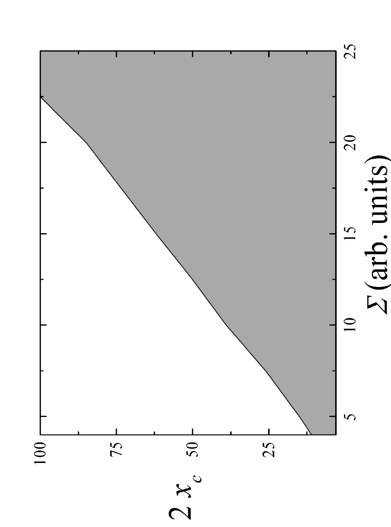
In order to understand the interplay of $\Sigma$ and $x_{c}$ better, we vary them independently and construct a phase plane $(\Sigma,x_{c})$ in Fig. 3. The separation of the region of patterns with large amplitude (displayed shadowed) from that of patterns of negligible amplitude is clear and occurs along a line of slope $9/2$ foot3 . This value of the slope is significant in light of the fact that in Fig. 2, the transition is seen at $\Sigma/L\approx 2/9.$ This clarifies that it is the finite domain size that imposes a cut-off on the Gaussians considered in Fig. 2, and that the domain size $L$ there plays the precise role of $2x_{c}$ in Fig. 3.

Figure 3: Separation of large-amplitude patterns (shadowed region) from negligible-amplitude patterns for the cut-off Gaussian influence functions with width $\Sigma$ and cut-off length $x_{c}$. The domain size is $L=100$. Units for $\Sigma$ and $x_{c}$ are arbitrary but identical.

The cut-off Gaussians or the square influence functions possess an abruptness feature which would not be present in a physical system. To ensure smoothness, we borrow from tsa and consider an influence function (for periodic boundary conditions)

$$f_{\sigma,\,r}(x) = \frac{1}{Z_{r}}[1-\frac{r\,x^{2}}{g(r,\sigma)}]^{1/r}\Theta(\xi_{c}-x)\Theta(\xi_{c}+x),$$

$$Z_{r} = \sqrt{\frac{\pi g(r,\sigma)}{r}}\frac{\Gamma(1/r+1)}{\Gamma(1/r+3/2)},$$

$$g(r,\sigma) = (2+3r)\sigma^{2}.$$ (6)

Here $r$ is non-negative, $\Gamma$ is the Gamma function, and the influence function has a cut-off at $\xi_{c}$ with

$$\xi_{c}=\sigma\sqrt{\frac{2+3r}{r}}.$$ (7)

Figure 4: Counterpart of Fig. 3 for the influence function of Eq. (6). Inset shows $f_{\sigma,\,r}$ in the periodic boundary condition case for several values of $r=100$ (dashed), $1$ (dotted), and $.01$ (full); respectively, $\Sigma=70$, $7$, and $.7$. The square and the Gaussian emerge as particular cases. Units as in Fig. 3.

The limit $r=0$ is the Gaussian. Note that $\xi_{c}$ denotes a natural cut-off of this function while $x_{c}$ in the Gaussian case is imposed externally by multiplying by a symmetric square function of width 2$x_{c}$. The width $\Sigma$, the range $\sigma$, and the parameter $r$ are related through

$$\Sigma=\xi_{c}\sigma(\xi_{c}^{2}-3\sigma^{2})^{-1/2}=\xi_{c}\sqrt{2r}.$$ (8)

It is also possible to define the function $f_{\sigma,\,r}$ for negative values of $r,$ specifically for $0>r>-2/3,$ through $f_{\sigma,\,r}(x,y)=\frac{1}{Z_{r}}\left[1-\frac{r(x-y)^{2}}{g(r,\sigma)}\right]^{1/r};\,Z_{r}=\sqrt{\frac{\pi g(r,\sigma)}{-r}}\frac{\Gamma(-1/r-1/2)}{\Gamma(-1/r)}$ as in ref. tsa , but analysis with such long-tailed $f_{\sigma,\,r}$’s does not add anything important to our present study, the results being similar to those for Gaussians. In addition to the smoothness property of these functions, they have the feature that they reduce to a square or a Gaussian in the respective limits $r\rightarrow 0$ and $r\rightarrow\infty$ (see inset in Fig. 4). It is therefore possible with their help to study for a given cut-off length the effect of varying the width (central curvature) and vice-versa. We fix a value of the natural cut-off $\xi_{c}$ well within the domain size $L$, and plot in Fig. 4 the counterpart of Fig. 3 for the class of influence functions given by Eq. (6). The two plots are similar in that the regions of large-amplitude and small-amplitude patterns are separated cleanly by what appears to be a straight line in the phase space. The slopes are different ($9/2$ for Fig. 3 but about $8$ for Fig. 4). We conclude that the cut-off length and the central curvature are both relevant to the formation of patterns in an interrelated manner shown by the phase plots. It should be noticed that while the Gaussian has an infinite cut-off $x_{c}$ and a finite width $\Sigma$, the square has a finite cut-off $x_{c}$ and an infinite width (curvature at center). Our introduction of Gaussians with an external cut-off provided in the first part of our investigation Gaussians wherein both control quantities were finite. Our introduction of the influence functions defined in Eq. (6) similarly provided square-like functions wherein both control quantities were finite. The inset of Fig. 4 makes it particularly clear that we can produce influence functions for this case with a fixed cut-off and $\Sigma$ ranging from $0$ to $\infty$.

We have performed a number of further studies of pattern formation from the long-range Fisher equation (2). They include extension to

Figure 5: Typical steady-state pattern in a 2D system with periodic boundary conditions and a cut-off influence function. Lighter areas correspond to larger values of $u$. Parameters are arbitrary.

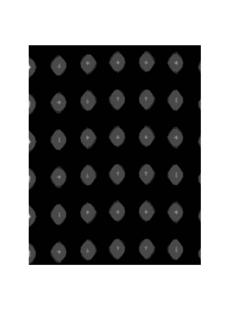
2-dimensional systems, typified by Fig. 5, in which patterns are shown for periodic boundary conditions and a cut-off function of the kind described in Eq. (6). We have also studied the effects of boundary conditions. As an example we display in Fig. 6 the lower-symmetry

Figure 6: Typical steady state patterns with cut-off influence function and zero-flux boundary conditions.

patterns for zero-flux conditions that appear to have additional modulation in the peaks. We have also investigated the time evolution of the patterns and found it to have considerable complexity even for simple initial conditions. We will report these various results elsewhere. Here we would like to draw attention to the features of the influence function, cut-off length and central curvature or width, whose ratio appears to determine whether the steady-state patterns have negligible or sizeable amplitude, the critical value of that ratio being different for different families of influence functions. We have systematized our numerical findings through the phase plots in Figs. 3 and 4. Our use of simple influence functions, such as the square, the Gaussian, and the cut-off Gaussian, as well as of richer functions as in ref. tsa which reduce to these forms, has resulted in our being able to focus on what features are responsible for what aspects of the patterns. We hope that future investigations will clarify at a basic level the picture presented by our numerical findings and make possible predictable manipulation of patterns in real systems such as bacterial colonies by controlling the influence function via control of the flow of nutrients and/or chemotactic substances.

I Acknowledgements

This work is supported in part by the Los Alamos National Laboratory via a grant made to the University of New Mexico (Consortium of The Americas for Interdisciplinary Science) and by National Science Foundation’s Division of Materials Research via grant No DMR0097204.

References

- (1) E. Ben-Jacob, I. Cohen and H. Levine. Adv. Phys. 49 ,395-554 (2000)
- (2) J. Wakita, K. Komatsu, A. Nakahara, T Matsuyama, M. Matsushita. Journ. Phys. Soc. Japan 63, 1205 (1994).
- (3) A. L. Lin, B. Mann, G. Torres, B. Lincoln, J. Kas and H. L. Swinney, "Localization and extinction of bacterial populations under inhomogeneous growth conditions", preprint.
- (4) D.R. Nelson and N.M. Shnerb, Phys. Rev. E 58,1383 (1998); K.A. Dahmen, D.R. Nelson and N.M. Shnerb, J. Math Biology, 41,1 (2000).
- (5) B. Mann, Spatial phase transitions in bacterial growth, Ph.D. Thesis (2001), unpublished.
- (6) R.A.Fisher, Ann. Eugen. London 7, 355-369 (1937).
- (7) C. T. Lee, M. F. Hoopes, J. Diehl, W. Gilliland, G. Huxel, V. Leaver, K. McCann, J. Umbanhowar and A. Mogilner, J. Theor. Biol. 201, 201-219 (2001).
- (8) A. Mogilner, L. Edelstein-Keshet, J. Math. Biol. 38, 534 (1999).
- (9) V. M. Kenkre, in Patterns, Noise, and the Interplay of Nonlinearity and Complexity, eds. V. M. Kenkre and K. Lindenberg, Proceedings of the PASI on Modern Challenges in Statistical Mechanics, AIP (2003).
- (10) Such a critical range does not appear in the zero-flux case.
- (11) The limits and correspond to no patterns as mentioned earlier.
- (12) C. Tsallis, J.Stat. Phys. 52, 449 (1988).