Noise-induced failures of chaos stabilization: large fluctuations and their control

Abstract

Noise-induced failures in the stabilization of an unstable orbit in the one-dimensional logistic map are considered as large fluctuations from a stable state. The properties of the large fluctuations are examined by determination and analysis of the optimal path and the optimal fluctuational force corresponding to the stabilization failure. The problem of controlling noise-induced large fluctuations is discussed, and methods of control have been developed.

Introduction

The control of chaos represents a very real and important problem in a wide variety of applications, ranging from neuron assemblies to lasers and hydrodynamic systems Boccalettia:00 . The procedure used consists of stabilizing an unstable periodic orbit by the application of precisely designed small perturbations to a parameter and/or a trajectory of the chaotic system. Different methods of chaos control have been suggested and applied in many different physical contexts, as well as numerically to model systems Boccalettia:00 . For practical applications of these control methods, it is important to understand how noise influences the stabilization process, because fluctuations are inherent and inevitably present in dissipative systems. The problem has not been well studied. Typically, a method is developed for stabilization of the orbit without initially taking any account of fluctuations. Only then do the authors check the robustness of their method by introducing weak noise into the system Boccalettia:00 . Thus, in the celebrated pioneering work of Ott, Grebogi and York, “Controlling chaos” Ott:90 , the authors just noted that noise can induce failures of stabilization.

In several works Bishop:96 ; Botina:97 methods are developed for the stabilization of unstable orbits in the presence of noise. They are based on a strong feedback approach to suppress any deviation from the stabilized states. There are also methods Collins:95 that use noise to move the system to a desired unstable state, and then stabilize it there.

In this work we consider noise-induced failures in the stabilization of an unstable orbit and the problem of controlling these failures. The method of Ott, Grebogi and Yorke (OGY) Ott:90 and a modification of the adaptive method (ADP) Boccalettia:00 are used to stabilize an unstable point of the logistic map. We consider the small noise limit where stabilization failures are very rare and can therefore they be considered as large fluctuations (deviations) from a stable state. We study the properties of large deviations by determining the optimal paths and the optimal fluctuational forces corresponding to the failures. We employ two methods to determine the optimal paths and forces. The first of these builds and analyzes the prehistory probability distribution to determine the optimal path and optimal force Dykman:92 . The second method considers an extended map (relative to the initial one) which defines fluctuational paths and forces in the zero-noise limit Graham:91 ; Grassberger:89 . Furthermore we use the optimal paths and forces to develop methods of controlling the large deviations, i.e. the noise-induced failures of stabilization.

In section I we describe the procedures for local and global stabilization of an unstable orbit of the logistic map. The general approach to the control of a large deviation is presented in section II. Noise-induced failures of local and global stabilization are considered in sections III and IV respectively. The results obtained are discussed in the conclusion.

I Chaos stabilization

For simplicity we will stabilize an unstable fixed point $x^{*}$ of the logistic map:

$$x_{n+1}=rx_{n}(1-x_{n}),$$ (1)

where $x_{n}$ is a coordinate, $n$ is discrete time and $r$ is the control parameter that determines different regimes of the map’s behavior (1). The coordinate of the fixed point $x^{*}$ is defined by the condition: $x_{n+1}=x_{n}$, and consequently its location depends on the parameter $r$:

$$x^{*}=1-\frac{1}{r}.$$ (2)

We set the parameter $r=3.8$, a value for which an aperiodic (chaotic) regime is observed (1), and the point $x^{*}$ is embedded in the chaotic attractor.

From the range of existing stabilization methods, we chose to work with just two: the OGY and ADP methods mentioned above.

To stabilize a fixed point by the OGY method, perturbations $\Delta r$ are applied to the parameter $r$, leading to the map being modified (1) in the following manner:

$$x_{n+1} = (r+\Delta r_{n})x_{n}(1-x_{n}),$$

$$\Delta r_{n}=r\frac{(2x^{*}-1)(x_{n}-x^{*})}{x^{*}(1-x^{*})}.$$

To stabilize a fixed point by the ADP method, perturbations $\Delta x$ are applied to the map’s coordinate. The value of the perturbation $\Delta x$ is defined by the distance between the current system coordinate and the coordinate of the stabilized state:

$$x_{n+1} = rx_{n}(1-x_{n})+\Delta x_{n},$$

$$\Delta x_{n}=(x_{n}-x^{*}).$$

The ADP method is simple to use in practice. Different modifications of the adaptive method are therefore used in many papers devoted to experiments on the control of chaos.

We consider two types of stabilization procedure: local stabilization and global stabilization.

During local stabilization, the perturbations $\Delta r$ and $\Delta x$ differ from zero only if the following condition is satisfied:

$$|x_{n}-x^{*}|<\epsilon.$$ (5)

Here $\epsilon$ is a small value: we fixed $\epsilon=0.01$. If the condition (5) is not satisfied then stabilization is absent, i.e. $\Delta r=0$ or $\Delta x=0$.

During global stabilization perturbations are switched on when the condition (5) is satisfied for the first time, and remain present for all future time.

So, local or global stabilization involve modifications of the initial map (1), and thus use another map in the form (I) or (I). The fixed point $x^{*}$ is an attractor of the new map. After the stabilization is switched on, a trajectory of the map tends to the fixed point $x^{*}$, and subsequently remains there.

In the presence of noise the trajectory fluctuates in the vicinity of the stabilized state, i.e. noise-induced dynamics appears. In addition, noise can induce stabilization failures. For local stabilization they imply a breakdown in the condition (5), and for global stabilization they correspond to an escape of the trajectory from the basin of attraction of the fixed point $x^{*}$.

Our aim is to study these noise-induced stabilization failures and analyze the problem of how to suppress them. We therefore consider the maps (I) and (I) in the presence of additive Gaussian fluctuations:

$$x_{n+1} = (r+\Delta r_{n})x_{n}(1-x_{n})+D\xi_{n},$$

$$\Delta r_{n}=r\frac{(2x^{*}-1)(x_{n}-x^{*})}{x^{*}(1-x^{*})},$$

$$x_{n+1} = rx_{n}(1-x_{n})+\Delta x_{n}+D\xi_{n},$$

$$\Delta x_{n}=(x_{n}-x^{*}).$$

Here $D$ is the noise intensity; and $\xi_{n}$ is a Gaussian random process with zero-average $\langle\xi\rangle=0$, delta-correlation function $\langle\xi_{n}\xi_{n+k}\rangle=\delta(k)$, and dispersion $\langle\xi^{2}\rangle=1$. We use a high-speed noise generator rt .

II Control of large fluctuations

Large fluctuations manifest themselves as large deviations from the stable state of the system under the action of fluctuational forces. Large fluctuations play a key role in many phenomena, ranging from mutations in DNA to failures of electrical devices. In recent years significant progress has been achieved both in understanding the physical nature of large fluctuations and in developing approaches for describing them. The latter are based on the concept of optimal paths – the paths along which the system moves during large fluctuations. Large fluctuations are very rare events during which the system moves from the vicinity of a stable state to a state remote from it, at a distance significantly larger than the amplitude of the noise. Such deviations can correspond to a transition of the system to another state, or to an excursion along some trajectory away from the stable state and then back again. During such deviations the system is moved with overwhelming probability along the optimal path under the action of a specific (optimal) fluctuational force. The probability of motion along any other (non-optimal) path is exponentially smaller. In practice, therefore large fluctuations must of necessity occur along deterministic trajectories. The problem of controlling large fluctuations can thus be reduced to the task of controlling motion along a deterministic trajectory. Consequently, the control problem can be solved through application of the control methods developed for deterministic systems Pontryagin .

Let us consider the control problem. Formally, the task that we face in controlling noise-induced large fluctuations consists of writing a functional $R$, the extrema of which correspond to optimal solutions of the control problem, i.e. solutions with minimal required energy Whittle:96 ; Rabitz:97 ; Smelyanskiy:97 . The form of the functional $R$ depends on a number of different additional conditions related to e.g. the system dynamics, the energy of the control force, or the time during which it is applied Whittle:96 ; Rabitz:97 ; Smelyanskiy:97 . We will follow the work Smelyanskiy:97 and consider the control of large fluctuations by a weak additive deterministic control force. Weakness means here that the energy of the control force is comparable with the energy (dispersion) of the fluctuations (see Whittle:96 for details). In this case, the extremal value of the functional $R$ for optimal control, which moves the system from an initial state $x^{i}$ to a target state $x^{f}$, takes the form Smelyanskiy:97 :

$$R_{\rm opt}(x^{f},F) = S^{(0)}(x^{f})\pm\Delta S,$$ (8)

$$\Delta S = (2F)^{1/2}\left[\sum_{k=N_{i}}^{N_{f}}(\xi_{k}^{\rm opt})^{2}\right]^{1/2};$$

where $\xi_{k}^{\rm opt}$ is the optimal fluctuational force that induces the transition from $x^{i}$ to $x^{f}$ in the absence of the control force; $S^{(0)}$ is an energy of the transition, $N_{i}$ and $N_{f}$ are the times at which the fluctuational force $\xi_{k}^{\rm opt}$ starts and stops , and $F$ is a parameter defining the energy of the control force.

The optimal control force $u_{n}^{\rm opt}$ for the given functional (8) is defined Smelyanskiy:97 by:

$$u_{n}^{\rm opt}= \mp (2F)^{1/2}\xi_{n}^{\rm opt}\left[\sum_{k=N_{i}}^{k=N_{f}}(\xi_{k}^{\rm opt})^{2}\right]^{1/2}$$ (9)

$$\times \delta(x_{n}-x_{n}^{\rm(0)opt})\,,$$

where $x_{n}^{\rm(0)opt}$ is the optimal fluctuational path in the absence of the control force. The minus sign in the expression (9) decreases the probability of a transition to the state $x^{f}$, and the plus sign increases the probability. It can be seen (9) that the optimal control force $u_{n}^{\rm opt}$ is completely defined by the optimal fluctuational force $\xi_{k}^{\rm opt}$, and the optimal fluctuational path $x_{n}^{\rm(0)opt}$, corresponds to the large fluctuation. Therefore to solve the control problem it is necessary, first, to determine the optimal path $x_{n}^{\rm(0)opt}$ leading from the state $x^{i}$ to the state $x^{f}$ under the action of the optimal fluctuational force $\xi_{k}^{\rm opt}$. Thus, a solution of the control problem depends on the existence of an optimal path: it is obvious that the approach described should be straightforward to apply, provided that the optimal path exists and is unique.

We consider below an application of the approach described to suppress large fluctuations in the one-dimensional map. The large fluctuations in question are considered here to correspond to failures in the stabilization of an unstable orbit.

The control procedure depends on the determination of the optimal path and optimal fluctuational force and, to define them, we will use two different methods. The first is based on an analysis of the prehistory probability distribution (PPD) and the second one consists of solving a boundary problem for an extended map which defines fluctuational trajectories.

The PPD was introduced in Dykman:92 to analyze optimal paths experimentally in flow systems. We will use the distribution to analyze fluctuational paths in maps. Note, that in Luchinsky:97 ; Khovanov:00 it was shown that analysis of the PPD allows one to determine both the optimal path and the optimal fluctuational force. The essence of this first method consists of a determination of the fluctuational trajectories corresponding to large fluctuations for extremely small (but finite) noise intensity, followed by a statistical analysis of the trajectories. In this experimental method the behaviour of the dynamical variables $x_{n}$ and of the random force $\xi_{n}$ are tracked continuously until the system makes its transition from an initial state $x^{i}$ to a small vicinity of the target state $x^{f}$. Escape trajectories $x_{n}^{\rm esc}$ reaching this state, and the corresponding noise realizations $\xi_{n}^{\rm esc}$ of the same duration, are then stored. The system is then reset to the initial state $x^{i}$ and the procedure is repeated. Thus, an ensemble of trajectories is collected and then the fluctuational PPD $p_{n}^{h}$ is constructed for the time interval during which the system is monitored. This distribution contains all information about the temporal evolution of the system immediately before the trajectory arrives at the final state $x^{f}$. The existence of an optimal escape path is diagnosed by the form of the PPD $p_{n}^{h}$: if there is an optimal escape trajectory, then the distribution $p_{n}^{h}$ at a given time $n$ has a sharp peak at optimal trajectory $x_{n}^{\rm opt}$. Therefore, to find an optimal path it is necessary to build the PPD and, for each moment of time $n$, to check for the presence of a distinct narrow peak in the PPD. The width of the peak defines the dispersion $\sigma_{n}^{h}$ of the distribution and it has to be of the order of the mean-square noise amplitude $\sqrt{D}$ Dykman:92 . The optimal fluctuational force that moves the system trajectory along the optimal path can be estimated by averaging the corresponding noise realizations $\xi_{n}^{\rm esc}$ over the ensemble. Note, that investigations of the fluctuational prehistory also allows us to determine the range of system parameters for which optimal paths exist.

To determine the optimal path and force by means of the second method we analyze extended maps Graham:91 ; Grassberger:89 using the principle of least action Grassberger:89 . Such extended maps are analogous to the Hamilton-Jacobi equation in the theory of large fluctuations for flow systems. For the one-dimensional map $x_{n+1}=f(x_{n})+D\xi_{n}$, the corresponding extended map in the zero-noise limit takes the form:

$$x_{n+1} = f(x_{n})+y_{n}/g(x_{n}),$$

$$y_{n+1} = y_{n}/g(x_{n}),$$ (10)

$$g(x_{n}) = \frac{\partial f(x_{n})}{\partial x_{n}}.$$

The map is area-preserving, and it defines the dynamics of the noise-free map $x_{n+1}=f(x_{n})$, if $y_{n}=0$. If $y_{n}\neq 0$ then the coordinate $x_{n}$ corresponds to a fluctuational path, and the coordinate $y_{n}$ to a fluctuational force. Stable and unstable states of the initial map become saddle states of the extended map. So, the fixed point $x^{*}$ of the ADP (I) and OGY (I) maps becomes a saddle point of the corresponding extended map. Fluctuational trajectories (including the optimal one) starting from $x^{*}$ belong to unstable manifolds of the fixed point $(x^{*},0)$ of the extended map.

The procedure for determination of the optimal paths consists of solving the boundary problem for the extended map (II):

$$x_{-\infty}=x^{*},~{}~{}~{}~{}~{}y_{-\infty}=0$$ (11)

$$x_{\infty}=x^{f},~{}~{}~{}~{}y_{\infty}=0;$$ (12)

where $x^{*}$ is the initial state and $x^{f}$ is a target state.

To solve the boundary problem different methods can be used. For the one-dimensional maps under consideration, a simple shooting method is enough numeric . We choose an initial perturbation $l$ along the linearized unstable manifolds in a vicinity of the point $(x^{*},0)$ of the map (II). The procedure to determine a solution can be as follows: looking over all possible values $l$, we determine a trajectory which tends to the point $(x^{f},0)$. Note that, because these maps are irreversible there exist, in general, an infinite number of solutions of the boundary problem. The optimal trajectory (path) has minimal action (energy) $S=\sum_{n=-\infty}^{\infty}y_{n}^{2}$; here $y_{n}$ is calculated along the trajectory, corresponding a solution of the boundary task.

III Noise-induced failures in local stabilization

A breakdown of the condition (5) corresponds to a failure of local stabilization, i.e. to the noise-induced escape of the trajectory from an $\epsilon$-vicinity of the fixed point $x^{*}$. The target state $x^{f}$ corresponds to the boundaries of the stabilization region: $x^{f}=x^{*}\pm\epsilon$.

Instead of analyzing the maps (I) and (I) in the $\epsilon$-vicinity of the fixed point $x^{*}$ we can investigate linearized maps of the following form:

$$x_{n+1} = ax_{n}+D\xi_{n};$$ (13)

here $a$ is a value of derivative $\partial f(x_{n})/\partial x_{n}$ in the fixed point $x^{*}$. For the map (I) the derivative is equal to zero $a_{\rm OGY}=0$, and for the map (I) $a_{\rm ADP}=-0.8$.

Let us investigate stabilization failure by considering the most probable (optimal) fluctuational paths, which lead from the point $x^{*}$ to boundaries $x^{*}\pm\epsilon$. For linearized maps (13) the extended map (II) can be reduced to the form:

$$x_{n+1}=ax_{n}+\frac{y_{n}}{a},$$ (14)

$$y_{n+1}=\frac{y_{n}}{a}$$

with the initial condition ($x_{0}=x^{*}$, $y_{0}=0$) and the final condition $x^{f}=x^{*}\pm\epsilon$. It can be seen that a solution of the map (14) increases proportionally to $y_{n}={\rm const}/a^{n}$ Reimann:91 . This means that, for the ADP map (I), the amplitude of the fluctuational force increases slowly but that, for the OGY map (I), the failure arises as the result of only one fluctuation (iteration). Because equation (14) is linear, the boundary problem will have a unique solution numeric . Thus, analysis of the linearized extended map (14) shows that there is an optimal path, and it gives a qualitative picture of exit through the boundary $x^{*}\pm\epsilon$.

Let us check the existence of the optimal paths through an analysis of the prehistory of fluctuations. To obtain exit trajectories and noise realizations we use the following procedure. At the initial moment of time, a trajectory of the map is located at point $x^{*}$. The subsequent behaviour of the trajectory is monitored until the moment at which it exits from the $\epsilon$-region of the point $x^{*}$. The relevant part of the trajectory, just before and after its exit, are stored. The time at which the exit occurs is set to zero. Thus ensembles of exit trajectories and of the corresponding noise realizations are collected and PPDs are built.

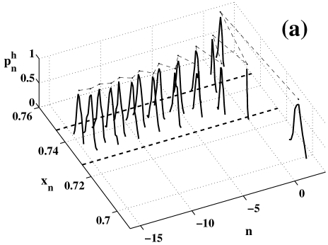
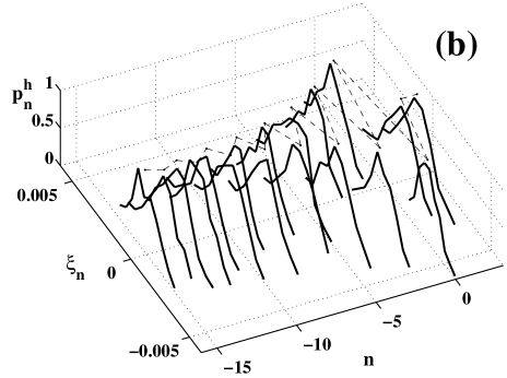
Figure 1: PPDs $p_{h}^{n}$ of the exit trajectories (a) and noise realizations (b) of ADP map for the boundary $(x^{*}-\epsilon)$. The thick dashed lines indicate $\epsilon$-region of stabilization. The thin dashed lines connect maxima of PPDs. The noise intensity is $D=0.0011$.

To start with, we will discuss these ideas in the context of the ADP map. Fig. 1(a) shows PPDs of the escape trajectories of the ADP map, and the corresponding noise realizations for the exit through the boundary $(x^{*}-\epsilon)$ are shown in Fig. 1(b). The picture of exit through the other boundary $(x^{*}+\epsilon)$ is symmetrical, so we present results for one boundary only. It is evident (Fig. 1) that there is the only one exit path. Note, that the path to the boundary $(x^{*}-\epsilon)$ is approximately 2.8$\times$ more probable than the path to the boundary $(x^{*}+\epsilon)$. This difference arises from an asymmetry of the map in respect of the boundaries.

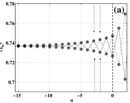
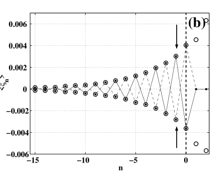
Figure 2: The optimal paths (a) and the optimal forces (b) for exit through the boundary $(x^{*}-\epsilon)$ (solid line) and the boundary $(x^{*}+\epsilon)$ (dashed line) for ADP map. Circles indicate the optimal paths and forces obtained by solving the boundary problem for the linearized extended map (14). The optimal paths and forces used in the control procedure are marked by arrows.

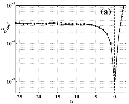
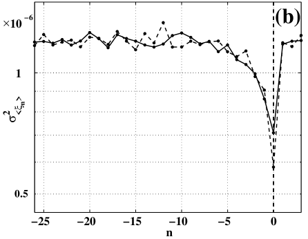
Figure 3: (a) The dispersion of the exit trajectories, and (b) the dispersion of the corresponding noise realizations for exit through the boundary $(x^{*}-\epsilon)$ (solid line) and the boundary $(x^{*}+\epsilon)$ (dashed line) for the ADP map.

Because for each boundary there is the only one exit path, the optimal path and the optimal fluctuational force can be determined by simple averaging of escape trajectories and noise realizations respectively. In Fig. 2 the optimal exit paths and the optimal fluctuational forces are shown for the boundaries $(x^{*}-\epsilon)$ and $(x^{*}+\epsilon)$. The paths and the forces coincide with a solution of the boundary problem (circles in the Fig. 2) of the extended linear map (14). The time dependence of the dispersion $\sigma_{n}^{h}$ of PPDs for the exit trajectories and noise realizations are shown in Fig. 3. As can be seen (Fig. 2) the optimal path is long, and the amplitude of the fluctuational force increases slowly, in agreement with analysis of the linearized map (14). The dispersion $\sigma_{n}^{h}$ of both trajectories and noise realizations decreases by construction as the boundary is achieved (Fig. 3).

The optimal fluctuational force obtained (Fig. 2(b)) must correspond Khovanov:00 to the energy-optimal deterministic force that induced the stabilization failure. We have checked this prediction and found that the optimal force induces the exit from an $\epsilon$-region of the point $x^{*}$: we selected an initial condition at the point $x^{*}$ and included the optimal fluctuational force additively; as a result we observed the stabilization failure. If we decrease the amplitude of the force by 5-10%, then the failure does not occur. It appears, therefore, the deduced force allows us to induce the stabilization failure with minimal energy (see Khovanov:00 for details).

Using the optimal path and the force we can solve the opposite task Whittle:96 ; Smelyanskiy:97 — to decrease the probability of the stabilization failures. Indeed, if during the motion along the optimal path we will apply a control force with the same amplitude but with the opposite sign as the optimal fluctuational force has, then, obviously, the failure will not occur. Because we know the optimal force then, in accordance with the algorithm Smelyanskiy:97 described above, it is necessary to determine the time moment when system is moving along the optimal path. For the ADP method the optimal path is long enough to identify that a trajectory is moving along the optimal path, and then to apply a control force.

In the presence of control the map (I) is modified:

$$x_{n+1} = rx_{n}(1-x_{n})+\Delta x_{n}+D\xi_{n}+u_{n},$$

$$\Delta x_{n}=(x_{n}-x^{*});$$

here $u_{n}$ is the deterministic control force.

We use the following scheme to suppress the stabilization failures. Initially the control force is equal to zero ($u_{n}=0$) and the map is located in the point $x^{*}$; we continuously monitor a trajectory of the map (III) and define the time moment when the system starts motion along the optimal path $\langle x_{n}\rangle$. We assume that the system moves along the optimal path $\langle x_{n}\rangle$ if it passes within a small vicinity of the coordinate $\langle x_{-2}\rangle$ and then within a small vicinity of $\langle x_{-3}\rangle$ (see arrows in Fig. 2(a)). Then on the following iteration we add the control force $u_{n}=-{\rm sign}(\xi_{n})\langle\xi_{n}\rangle$, $n=-1$ (see Fig. 2(b)).

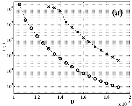
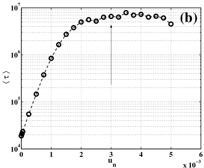
Figure 4: (a) The dependences of mean time $\langle\tau\rangle$ between stabilization failures on noise intensity $D$ in the absence (circles) and in the presence (crosses) of the control. The size of the stabilization region is $\epsilon=0.01$. (b) The dependence of the mean time $\langle\tau\rangle$ on the amplitude of the control force $u_{n}$ is presented for the ADP method. The value of $\langle\tau\rangle$ corresponding to the optimal fluctuational force is marked by the arrow.

In Fig. 4(a) dependences of the mean time $\langle\tau\rangle$ between the failures on the noise intensity $D$ are plotted in the absence, and in the presence, of the control procedure. It is clear that the mean time $\langle\tau\rangle$ is substantially increased by the addition of the control, i.e. stability in the face of fluctuations is significantly improved by the addition of the control scheme. The efficiency of the control procedure depends exponentially Smelyanskiy:97 on the amplitude of the control force (Fig. 4(b)), and there is an optimal value of the control force, which is very close to the value (arrow in Fig. 4(b)) of the optimal fluctuational force.

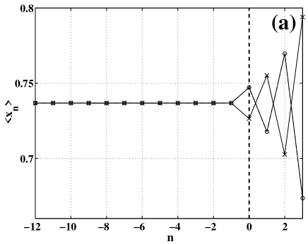
Figure 5: For the OGY map, the optimal path (a) and the optimal force (b) are shown for exit through the boundary $(x^{*}-\epsilon)$ (crosses) and the boundary $(x^{*}+\epsilon)$ (circles).

Now consider noise-induced stabilization failures for OGY map (I). An analysis of the linearized map has shown that the failure occurs as the result of a single fluctuation. We have checked the conclusion by an analysis of the fluctuational trajectories of the map (I), much as we did for the ADP map. The optimal path and optimal force are shown in Fig. 5 for both boundaries, $(x^{*}+\epsilon)$ and $(x^{*}-\epsilon)$. An exit occurs during one iteration and there is no a prehistory before this iteration. It means that we cannot determine the moment at which the large fluctuation starts and, consequently, that we cannot control the stabilization failures. The existence of a long prehistory is thus a key requirement in the control the large fluctuations.

We can of course decrease the probability of a failure by increasing the $\epsilon$-region of stabilization. The maximum possible increase would correspond to infinite boundaries – in which case we would be dealing with global stabilization.

IV Noise-induced failures of global stabilization

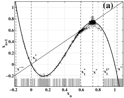
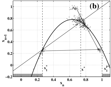
Figure 6: The OGY map (a) and the ADP map (b) on the plane $(x_{n}-x_{n+1})$ are shown by the thick solid line. Basins of attraction of the fixed point $x^{*}$ (white regions) and the attractor at infinity (black regions) are shown at the bottoms of the figures. The dashed lines indicate locations of the fixed points of the maps and the points defining the basin boundaries. Escape trajectories are shown by dots. The thin line in figure (b) corresponds to the optimal path.

To investigate fluctuational dynamics in the global stabilization regime, we consider the dynamics of the maps (I) and (I) with initial conditions at the fixed point $x_{0}=x^{*}$. We will first consider them in the absence of noise. The maps are shown on the plane $x_{n}-x_{n+1}$ in the Fig. 6.

The map (I) (Fig. 6(a)) has three fixed points of period one: the point $x^{*}\approx 0.7368$ is stable with the multiplier $\mu=0$; the points $x^{*}_{2}=0$ and $x^{*}_{1}\approx 0.5906$ are unstable with multipliers $\mu\approx-3.04$ and $\mu\approx 1.8016$, respectively. The map has two attractors: the point $x^{*}$ and the attractor at infinity . Their basins of attraction (Fig.6 (a)) are self-similar (fractal) Kaneko:83 ; Takesue:84 . The point $x^{*}_{1}$ and its pre-images by backward iteration lie on the basin boundaries of the attractors Grebogi:87 . In the intervals $x\in(-0.183,0.5906)$ and $x\in(0.862,1.027)$ the basins of the attractors alternate and are of different length. The interval $x\in(0.5906,0.862)$ corresponds to the widest basin of the fixed point $x^{*}$. The boundaries of this basin are defined by the unstable point $x^{*}_{1}$ and its pre-image $x^{I*}_{1}$. The semi-infinite intervals $x\in(-\infty,-0.183)$ and $x\in(1.027,\infty)$ correspond to basins of the attractor at infinity. The boundaries of the semi-infinite intervals are defined by the points $x^{-\infty}=-0.183$ and $x^{\infty}=1.027$, which correspond to the cycle of period 2.

The map (I) (Fig. 6(b)) has two fixed points: the point $x^{*}\approx 0.7368$ is stable with multiplier $\mu\approx-0.8$; and the point $x^{*}_{1}\approx 0.2632$ is unstable with multiplier $\mu\approx 2.8$. The map has two attractors: the fixed point $x^{*}$ and the attractor at infinity. The basins of attraction are smooth (Fig. 6 (b)). The first boundary of the basins is the point $x^{*}_{1}$ and the second boundary is a pre-image $x^{I*}_{1}$ of the point $x^{*}_{1}$.

So, each of the maps has two attractors, but the structure of their basins of attraction are qualitatively different.

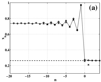
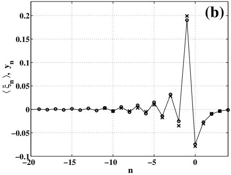
Figure 7: The optimal path (a) and the optimal force (b) obtained by experimental analysis of the PPD for the ADP map (I) (crosses) and by solving the boundary problem for the map (IV) (circles).

We now consider these maps (I) and (I) in the presence of noise. Noise can induce escape from the basin of the fixed point $x^{*}$, corresponding to failure of the stabilization. As before we examine the dynamics of the escape trajectories obtained for extremely small noise intensity in order to determine the optimal path and the optimal force. Fluctuational escape trajectories of the map (I) are shown by dots on the plane $(x_{n}-x_{n+1})$ in Fig. 6(b). As can be seen, there is one escape path, and the escape trajectories pass through the unstable point $x^{*}_{1}$. In Fig. 7 the optimal path and the optimal force obtained by averaging the escape trajectories and noise realizations respectively are shown by crosses. The stabilization failure clearly possesses a long prehistory. From the point of view of the control procedure, the presence of a large deviation of the system coordinate $\langle x_{n}\rangle$ at the time moment $n=-1$, and the smaller deviation of the fluctuational force $\langle\xi_{n}\rangle$ at the next time moment ($n=0$), are important.This is because the first fluctuation of coordinate $x_{n}$ can easily be identified and distinguished from non-optimal fluctuations in the vicinity of the stable state $x^{*}$.

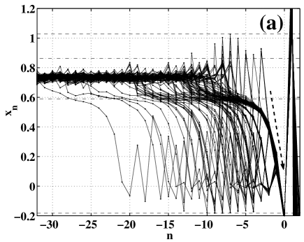
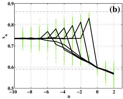
Figure 8: 100 escape trajectories of the OGY map collected in a vicinity of (a) the point $x^{-\infty}$ and (b) the point $x^{*}_{1}$. The size of the vicinity is defined as the mean square of noise intensity $D$. The dash-dot lines indicate the location of the boundary point $x^{*}_{1}$ and its pre-image $x^{I*}_{1}$; the dashed lines in (a) represent boundaries of the basins with fractal structure, i.e. of the points $x^{-\infty}$ and $x^{\infty}$. The thick lines in (b) correspond to different escape paths; the grey dots are coordinates of escape trajectories. The noise intensity is $D=0.018$.

Next, we examine the process of escape for the map (I). Fig. 8(a) shows escape trajectories superposed at the time moment when the trajectory crosses the basin boundary at the point $x^{-\infty}$. It is evident that there is no selected escape path. The escape trajectories can be divided into several groups with different probabilities. With maximum probability (almost 50%) the escape trajectories follow the arrowed path in Fig. 8(a)) corresponding to motion in the direction of the point $x^{-\infty}$ without any jumps in the opposite direction. The other paths include jumps in the opposite direction. The width of the distribution of fluctuational paths is comparable with the noise amplitude and there is no a specific fluctuational force. In Fig. 6(a) the escape trajectories are shown on the plane $(x_{n}$ – $x_{n+1})$. Is can be seen that, after the point $x_{1}^{*}$, the escape trajectories are located close to the trajectories of deterministic map, so we can suppose that after the point $x_{1}^{*}$ the motion has the character of directed diffusion. The interval between the points $x_{1}^{*}$ and $x^{-\infty}$ lies within the fractal basin, and this fact implies a variety of escape paths. Indeed, within a small vicinity of the point $x_{1}^{*}$ there is a piece of basin of the attractor at infinity. For escape, therefore, it is enough to bring the trajectory only to this basin. However, the size of this basin is small and a weak fluctuation can of course move the trajectory back to the basin of point $x^{*}$ and vice versa. As a result, the trajectory can spend a long time in the vicinity of the point $x_{1}^{*}$: it can return to the point $x^{*}$, as well as escape from the basin of the point $x^{*}$.

Thus, the fractal structure in the basin of attraction leads to complex behaviour of the escape trajectories; they can spend a long time in the fractal basin; motion in the direction of the attractor at infinity has the largest probability.

Investigations of escape from the point $x^{*}$ to the vicinity of the point $x_{1}^{*}$ have shown (Fig. 8(b)), that there is no specific path within this interval, so that we cannot determine the optimal path or the optimal force using an analysis of the escape trajectories. It is possible to select several different favoured paths (thick lines in the Fig. 8(b)), but dispersion of the trajectories for each of them is much larger than the noise intensity used.

We now determine the escape optimal paths and the forces by solving the boundary problems (11) and (12) for the extended maps:

$$x_{n+1} = f(x_{n})+y_{n}/g(x_{n}),$$

$$y_{n+1} = y_{n}/g(x_{n}),$$ (16)

$$f(x_{n}) = (r+\Delta r_{n})x_{n}(1-x_{n}),$$

$$g(x_{n}) = \frac{\partial f(x_{n})}{\partial x_{n}}$$

and

$$x_{n+1} = f(x_{n})+y_{n}/g(x_{n}),$$

$$y_{n+1} = y_{n}/g(x_{n}),$$ (17)

$$f(x_{n}) = rx_{n}(1-x_{n})+\Delta x_{n},$$

$$g(x_{n}) = \frac{\partial f(x_{n})}{\partial x_{n}},$$

which correspond to the maps (I) and (I). In such a way we have used the extended map (14) to analyze the linearized map (13).

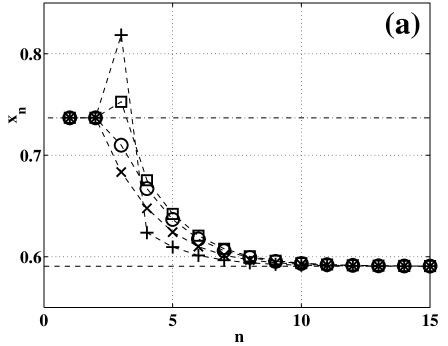
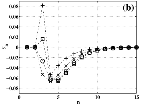
Figure 9: The optimal paths (a) and optimal forces (b) obtained by solution of the boundary problem for the OGY map. The path $t_{1}$ is marked with $\circ$, $t_{2}$ — $\Box$, $t_{3}$ — $\times$, $t_{4}$ — $+$.

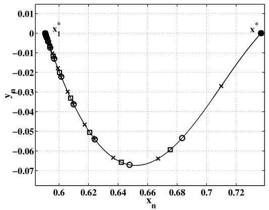
Figure 10: The stable manifold of the point $x^{*}_{1}$ of the OGY map. The symbols indicate the different optimal paths, using the same coding as in Fig. 9.

First, we consider the results of solving the boundary problem for the extended map (IV). To do so, we use a shooting method, with boundary conditions (11) and (12), where $x^{f}=x^{*}_{1}$. Since the derivative $g(x_{n})=\frac{\partial f(x_{n})}{\partial x_{n}}$ of the map (I) at the point $x^{*}$ is equal to zero, we cannot calculate eigenvectors of the point $(x^{*},0)$ of the map (IV). Therefore, as a parameter of the boundary problem we choose an initial perturbation $y_{0}$, since it defines all the trajectories going away from the point $(x^{*},0)$. Four solutions of the boundary problem, obtained numerically, are found to have practically the same action $S$. Four escape paths and noise realizations ($t_{1}-t_{4}$) of the map (IV) corresponding to these solutions are shown in Fig. 9. The trajectory $t_{4}$ has the minimum activation energy $S\approx 0.0115$ and the energies of other trajectories are practically the same: $S\approx 0.0123$. All the optimal trajectories lie on a stable manifold of the point ($x_{1}^{*},0$), and the stable manifold goes to the point ($x^{*},0$) (Fig. 10). If we take into account the fact that the noise intensity is finite during the experimentally analysis of escape trajectories (Fig. 8), then the fluctuational trajectories of the map (I) form a wide bunch around the optimal paths and trajectories can go along different the optimal paths at different time intervals. Thus, for the OGY map (I), the only way to determine optimal paths and forces is by solution of the boundary problem for the extended map, whereas an analysis of the PPD is not successful.

Now, let us consider the solution of the boundary problem for the map (IV). We have defined an unstable direction of the point $(x^{*},0)$ and used the length of a vector $l$ along this direction as a parameter of the boundary problem. There is just one solution for which the value of action $S=0.0449$, which is slightly smaller than the value $S=0.493$ calculated by using the PPD. The corresponding optimal path and optimal force are shown in Fig. 7 together with the path and the force found by using PPD. It can be seen (Fig. 7), that the optimal paths and the forces obtained by calculated PPD and by using the extended map are practically the same.

Thus, we have defined the optimal path and the optimal force corresponding to global stabilization failures, and we have compared two methods for determination of the optimal path and force: the first method being based on an experimental analysis of the prehistory probability distribution, and the second one being based on solving the boundary problem for an extended area-preserving map. The latter method allows us to determine the optimal path and force for both the maps (I) and (I) whereas experimental analysis of prehistory probability is only successful for ADP map (I).

Because there is no an unique escape path for the OGY map, it is impossible to apply the algorithm described above for controlling stabilization failures. We note however that, since we know the dynamics of the fluctuational trajectories, it is still possible to realize control of the fluctuations by using another approach. For example, a control force can be added whenever the system comes to the vicinity of the point $x_{1}^{*}$. In this case, however, the size of the vicinity and the magnitude and form of the control force are ill defined.

For stabilization of the ADP map, the opposite situation applies: there exist an unique optimal path and a corresponding optimal force. Consequently, we can realize a procedure for the control of large fluctuations. It is similar to that described above for local control. We monitor trajectories of the map (I) to identify the large deviation ($\langle x_{n}\rangle$, $n=-1$ in Fig. 7) and in the next iteration we add the control force $u_{n}=-\langle\xi_{n}\rangle$, $n=0$. The dependences on noise intensity $D$ of the mean time $\langle\tau\rangle$ between stabilization failures in the absence and in the presence of control are shown in Fig. 12(a). The dependence of $\langle\tau\rangle$ on the amplitude of the control force is shown in Fig. 12(b). The suggested control procedure is evidently effective.

Conclusion

We have considered noise-induced failures in the stabilization of an unstable orbit, and the problem of how to control such failures. In our investigations, they correspond to large deviations from stable points. We have examined two types of stabilization, local and global, and therefore analyzed fluctuational deviations of different size. We have shown that, for local stabilization, noise-induced failures can be analyzed effectively in terms of linearized noisy maps.

Large noise-induced deviations from the fixed point in one-dimensional maps have been analyzed within the framework of the theory of large fluctuations. The key point of our consideration is that the dynamics of the optimal path, and the optimal fluctuational force, correspond directly to stabilization failures. We have applied two approaches – experimental analysis of the prehistory probability distribution and the solution of the boundary problem for extended maps – to determine the optimal path and the optimal fluctuational force, and we have compared their results. For local stabilization, the two approaches give the same results. For global stabilization, however, the solution of the boundary problem enabled the optimal path and optimal fluctuational force to be determined for both the OGY and ADP maps, whereas investigation of fluctuations’ prehistory gave the optimal path and force for the ADP map only.

A procedure for the control of large fluctuations in one-dimensional maps has been demonstrated. It is based on the control concept developed in Smelyanskiy:97 for continuous systems. We have introduced an additional control scheme which significantly improves the stabilization of an unstable orbit in the presence of noise. It was successful for the ADP method of stabilization, and problematic for the OGY method. We have shown that the control procedure has limitations connected with the existence of unique optimal path and the presence of long time prehistory of large fluctuation. The relationships between the large fluctuation dynamics and the control procedures are summarized in Table I.

The considering of the control problem is relevant to a continuous system which has one-dimensional curve in the Poincare section, for example, to the Rossler system. For such a continuous system we can formulate the task of control as a control in discrete time moments (moments of intersection of the Poincare section) by using impulse actions. Intervals between the moments were used to calculate and to form a control force. Note, that the similar approach is wide used in control technique.

The present control approach has limitations which consist of necessity of studying the fluctuational dynamics of systems before considering of the control problem. Such studying can be done with use of extended maps of system, if it is known a system model, and/or experimentally by fluctuation prehistory analysing. For the local stabilization a system model can be easily written down by determination of eigen-value of a stabilized unstable point; there are a lot of effective methods to do it RMP . For the global stabilization there is no such a way and we need to investigate the fluctuation prehistory. Our investigations have shown that in this case we can met problems of determination of the control force. Indeed, we have shown that for the global stabilization of OGY map there are several most-probable escape paths with, practically, the same energy. As the result, a real escape path can be a combination of the different most-probable paths, so an escape trajectory does not go along a defined path as for the ADP map. Moreover, we can not determine the fluctuational force and, consequently, the control force, since we use for it averaging fluctuational trajectories which follow along an unique path. So, the control procedure is inapplicable. It is obviously, that for succesful control we have to change the control strategy. For example, we can try to predict a fluctuational action locally whereas now we try to know the full fluctuational dynamics. The local prediction can be based on a combination of real time prehistory analysis and reconstruction of the extended system Smel_PC .

Additionally, noise-induced escape through fractal boundaries has been studied in a one-dimensional map. It was found that fluctuational motion across fractal basins has a non-activation character. It was also established that there are several optimal escape paths from the fixed point of the OGY map (I) whereas, for the ADP map (I), the escape path is unique. We infer that the existence of several paths in the OGY map (I) is connected with the fact that the stable manifold of the boundary point $(x_{1}^{*},0)$ goes to the fixed point $(x^{*},0)$.

	Type of stabilization
	ADP	OGY	ADP	OGY
	local	local	global	global
Unique Optimal Path	X	X	X
Long Prehistory	X		X	X
Successful Control	X		X

Table 1: The relationships between the dynamics of fluctuational paths and the control procedures.

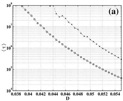
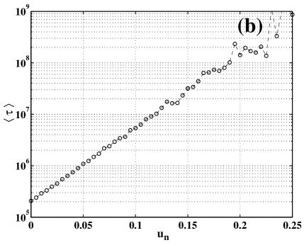
Figure 11: (a) Dependences of the mean time $\langle\tau\rangle$ between stabilization failures on noise intensity $D$ in the absence (circles) and in the presence (crosses) of the control. The stabilization is global, using the ADP method. (b) Dependence of the mean time $\langle\tau\rangle$ on the amplitude of the control force $u_{n}$.