Multi-site H-bridge breathers in a DNA–shaped double strand

Abstract

We investigate the formation process of nonlinear vibrational modes representing broad H-bridge multi–site breathers in a DNA–shaped double strand. Within a network model of the double helix we take individual motions of the bases within the base pair plane into account. The resulting H-bridge deformations may be asymmetric with respect to the helix axis. Furthermore the covalent bonds may be deformed distinctly in the two backbone strands. Unlike other authors that add different extra terms we limit the interaction to the hydrogen bonds within each base pair and the covalent bonds along each strand. In this way we intend to make apparent the effect of the characteristic helicoidal structure of DNA. We study the energy exchange processes related with the relaxation dynamics from a non-equilibrium conformation. It is demonstrated that the twist-opening relaxation dynamics of a radially distorted double helix attains an equilibrium regime characterized by a multi-site H-bridge breather.

PACS numbers: 87.-15.v, 63.20.Kr, 63.20.Ry

1 Introduction

Studies of chemical and physical properties of DNA have attracted considerable interest among physicists and biologists because of their relevance for a variety of biological processes, such as DNA transcription, gene expression and regulation and DNA replication [1]. In the context of the transcription process, the coding sequence on a DNA strand has to be made accessible to the RNA polymerase which necessitates that hydrogen bonds connecting the two strands have to be (temporarily) broken so that the DNA strands separate. This melted segment of DNA encloses $15-20$ opened base pairs and is called the transcription bubble.

The opening of the DNA molecule is a very complex process and a comprehensive explanation of the actual mechanisms underlying the observed dynamical processes is still to come. To tackle the problem of DNA dynamics nonlinear models of the DNA double helix have been proposed during the past two decades [2]-[6]. Different from molecular dynamics simulation methods, for which a great deal on the detailed reproduction of the molecular DNA structure is spent, the nonlinear models focus on the most relevant structural features only. The strength of the rather abstract nonlinear models of DNA lies then in the straightforward manner in which their soliton and breather solutions reproduce the prevalent dynamical behavior related with the strong energy localization and stable energy transport observed experimentally during the transcription process.

To model the base pair opening in DNA, Peyrard and Bishop (PB) proposed a planar ladder-like model of DNA assigning each base pair a vertical inter-strand vibrational degree of freedom simulating the stretchings and compressions of the corresponding H-bridges [2]. The binding forces of the hydrogen bridges are described by a Morse potential. The bases itself are treated as point masses. Horizontally, the bases on the same strand are coupled via the covalent interaction described by harmonic potentials. The PB has been extensively studied and localized oscillating solutions (breathers) and moving localized excitations [12] have been found reflecting successfully some typical features of the DNA opening dynamics such as the magnitude of the amplitudes and the time scale of the breathing of the ’bubble’ occurring prior to thermal denaturation [2]. In addition, studies in the context of thermal denaturation have been based on the PB model incorporating a heat bath [14]-[16].

Typical for many biomolecules is their interplay between functional processes and structural transitions [1]. In this respect the transcription process relying on the opening of DNA represents a prominent example. Indeed, it has been found that the bubble formation is strongly correlated with twist deformations and local openings are always connected with a local untwist of the double helix [6],[5],[7]. In order to account for the helicoidal structure of DNA the PB model has been significantly extended by Barbi, Cocco and Peyrard (BCP) [6]. In their model of a more realistic description of DNA, two degrees of freedom per base pair are introduced. There is a radial variable measuring the distance between two H-bridged bases along a line that connects them in the base plane being perpendicular to the helix axis. Further, the twist angle between this connecting line and a reference direction determines the orientation of the H-bridge. The twist-opening dynamics is described by radial breather solutions combined with kink-like solutions in the angular variable which have been constructed with the help of a multiple scale expansion technique [6].

In the current study of the nonlinear dynamics related with the opening process in DNA our aim is twofold. First of all, we study the energy exchange processes and the relaxation dynamics in DNA molecules after their excitation into a non-equilibrium conformation. Such an investigation is associated with recent mechanical experiments performed with single DNA molecules [17]-[21] forced away from their equilibrium conformations. After force applications energy redistribution within the DNA molecule takes place such that a new equilibrium conformation is attained [22]. Furthermore, for strong enough radial forces the mechanical unzipping of single DNA molecules is achievable [20]. We remark that for the current study our assumption is that the DNA molecules are imposed to not too strong external radial forces excluding the (immediate) separation of the strands. Secondly, besides the relaxation dynamics within B-DNA whose two strands are supposed to have been pulled apart in a certain region, we direct our attention on the formation of oscillating bubbles occurring previous to denaturation. In particular, within a nonlinear model approach we aim for the creation of multi-site radial breathers, which, compared with the one-site breather solutions obtained in [6],[7], provide stronger opening of an fairly extended segment of the DNA reproducing the experimentally observed oscillating bubbles involving $15-20$ base pairs.

The structure of the double helix of B-DNA is modeled by a steric network of oscillators in the frame of the base pair picture [2],[6] taking into account deformations of the hydrogen bond within a base pair and twist motions between adjacent base pairs. In augmentation of the oscillator model for the helicoidal DNA structure introduced in [6] we allow for individual motions of the bases within the base pair plane such that the vibrations of the H-bridges are no longer exclusively symmetric with respect to the helix axis unlike the symmetric radial motions considered in [6].

It is worth mentioning that when constructing helical variants of the Peyrard–Bishop model, the description of the hydrogen-bridge and covalent bonds is fairly clear: an asymmetric soft potential for the hydrogen bonds and harmonic terms for the covalent bond, in the hypothesis that the latter are more rigid and therefore the oscillations are small. It is not so evident how to model the stacking interaction in a straightforward manner. The physical origin of it lies in the bonds between overlapping bases, but these do not appear explicitly in the model. Different heuristic solutions have been tried as it will be commented in more detail later with interesting results. Here we focus on other aspects of the problem and take the helical shape of the DNA as given and add no extra term to maintain it. In this way we pretend to explore the effect of the helical shape in itself. The results are remarkable, the helical shape provides a change of the type of the effective coupling bringing about the possibility of stable multi–site H-bridge breathers, which have to be differentiated from broad one-site breathers. In this way much larger openings of the double strand are possible.

The paper is organized as follows: In the second section we describe our extended steric network model for the helical structure of the double helix of B-DNA. The third section deals with the relaxation dynamics within B-DNA molecules forced into locally distorted configurations and the fourth section is devoted to the construction of multi-site radial breathers. In the fifth section we discuss the linear modes of the breathers and their relation to the spectral features of the localized solutions. Finally, we present our conclusions.

2 Oscillator model for the helical structure of DNA

In our DNA model we incorporate the basic geometrical features of the DNA double helix structure which are essential to model the nonlinear dynamics of the twist-opening process. Similar to the approach in [6], we treat the right-handed helical form of B-DNA, which is a polymeric molecule composed of two coiled strands of nucleotides forming a double helix, as a helical double-stranded oscillator system. The constituents of the latter represent the nucleotides which are regarded as single nondeformable entities. Thus, no inner dynamical degrees of freedom of the nucleotides are taken into account which is justified by the time scale separation between the small-amplitude and fast vibrational motions of the individual atoms and the slower and relatively large-amplitude motions of the atom groups constituting the nucleotides [1]. Concerning the structural components, each nucleotide is composed of a sugar, a phosphate and a base. The sugar-phosphate groups of neighboring nucleotides on the same strand are linked via covalent bonds establishing the interaction related with the rigid backbone to the strand. There is a base attached to every sugar. Since, for simplicity, we do not distinguish between the four different types of bases, the nucleotides are considered as identical objects of fixed mass. Two bases on opposite strands are linked via hydrogen bonds holding the two strands of DNA together.

In the BCP twist-opening model, based on the base pair picture of DNA, the helicoidal structure of DNA has been conveniently described in a cylindrical reference system where each base pair possesses two degrees of freedom, namely a radial variable measuring the distance between a base and the central helix axis (viz., deformations of the corresponding H-bridge) and the angle with a reference axis in a plane perpendicular to the central axis which defines the twist of the helix [6].

Our model approach of the structural dynamics of the helicoidal DNA models is inspired by the ones used in Ref. [5]–[10], but differs from them in two important points: a) We release the constraint that the two bases in a base pair perform solely vibrational variations of the hydrogen bond length symmetric to the central axis along a line which connects the two bases crossing the central helix axis; b) Those models introduce for convenience extra potential terms which we discard because of the following reasons: On the one hand, not only they are sufficiently justified on physical grounds. On the other hand, we are interested in the effect of the helical structure on breather formation and try to keep the model as simple as possible to avoid masking the dynamical behavior. These differences will bring about remarkable consequences on multibreather stability and on the phonon spectrum as will be shown in the next sections. We also neglect vertical movements as Ref. [10] shows that they are not significant. Therefore, we extend the BCP model in the sense that we treat the two H-bridged strands individually and take individual two-dimensional equilibrium positions as well as displacement coordinates of a base within its base pair plane into account. As a consequence, the line connecting the two bases of a base pair, which is supposed to coincide with the orientation of the hydrogen bridge, does not necessarily intersects the central axis as distinct from the BCP model. In other words, for the equilibrium configuration of the double helix the two bases of a base pair may be positioned asymmetrically in radial direction and may be rotated also by different angles around the helix axis allowing for the simulation of polymorphic helical DNA matrices deviating from the perfectly regular equilibrium helix structure. In fact, real DNA molecules exhibit random structural imperfections of their equilibrium double helix caused by external and internal influencing factors such as the distorting impact of the solvent environs. Moreover, with our approach the DNA lattice dynamics can be initialized with arbitrary excitation patterns connected with individual displacements of each base different from the symmetric H-bridge deformations discussed previously in [6].

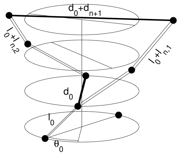
Figure 1: Schematic representation of the helicoidal structure of the DNA model.

We describe the double helix structure in a Cartesian coordinate system whose $z-$axis corresponds to the central helix axis as sketched in Fig. 1. The base pairs are situated in planes perpendicular to the central helix axis and the vertical distance between two consecutive planes is given by $h$. For the equilibrium configuration of B-DNA each base, with equilibrium coordinates $x_{n,i}^{(0)}$ and $y_{n,i}^{(0)}$, is rotated around the central axis by an angle $\theta_{n,i}^{(0)}$. The index pair $(n,i)$ labels the $n$-th base on the $i-$th strand with $i=1,2$ and $1\leqq n\leqq N$ , where $N$ is the number of base pairs considered. The equilibrium distance between two bases within a base pair, $d_{0}$, is determined by

$$d_{0}=\sqrt{\left(\,d_{n}^{x}\,\right)^{2}\,+\,\left(\,d_{n}^{y}\,\right)^{2}}\,,$$ (1)

where $d_{n}^{x}=\,x_{n,1}^{(0)}-x_{n,2}^{(0)}$ and $d_{n}^{y}=\,y_{n,1}^{(0)}-y_{n,2}^{(0)}$ are the projections of the line connecting the two bases on the $x,y-$axes of the coordinate system. The deviations $d_{n}$ from $d_{0}$ through displacements, $x_{n,i}$ and $y_{n,i}$, of the bases from their equilibrium positions, $x_{n,i}^{(0)}$ and $y_{n,i}^{(0)}$, are expressed as

$$d_{n}=\sqrt{\left(\,d_{n}^{x}+x_{n,1}-x_{n,2}\right)^{2}\,+\,\left(\,d_{n}^{y}+y_{n,1}-y_{n,2}\right)^{2}}-d_{0}\,.$$ (2)

For later use we introduce the quantity

$$\theta_{n}=\arctan\frac{d_{n}^{y}+y_{n,1}-y_{n,2}}{d_{n}^{y}+x_{n,1}-x_{n,2}}+2\,m\,\pi\,,$$ (3)

as the angle between the $x-$axis (as the reference direction) and the line connecting two (displaced) bases of a base pair measuring the alignment of the related H-bridge, $m$ being a integer to assure the monotonicity of $\theta_{n}$ with respect to $n$.

The three-dimensional equilibrium distance between two adjacent bases on the same strand is given by

$$l_{0}=\sqrt{h^{2}+\left(\,x_{n,i}^{(0)}-x_{n-1,i}^{(0)}\right)^{2}\,+\,\left(\,y_{n,i}^{(0)}-y_{n-1,i}^{(0)}\right)^{2}}\,,$$ (4)

and deviations from $l_{0}$ are determined by

$$l_{n,i}=\sqrt{h^{2}+\left(\,L_{n,i}^{x}+x_{n,i}-x_{n-1,i}\right)^{2}\,+\,\left(\,L_{n,i}^{y}+y_{n,i}-y_{n-1,i}\right)^{2}}-l_{0}\,,$$ (5)

with $L_{n,i}^{x}=x_{n,i}^{(0)}-x_{n-1,i}^{(0)}$ and $L_{n,i}^{y}=y_{n,i}^{(0)}-y_{n-1,i}^{(0)}$. The Hamiltonian of our model is then of the form

$$H=E_{kin}+U_{h}+U_{c}\,,$$ (6)

where $U_{h}$ and $U_{c}$ represent the potential energy part for the H-bond and the covalent bonds, respectively. The kinetic energy is determined by

$$E_{kin}=\frac{1}{2m}\,\sum_{i=1,2}\,\sum_{n=1}^{N}\,\left[\,\left(p_{n,i}^{(x)}\right)^{2}+\left(p_{n,i}^{(y)}\right)^{2}\right]\,,$$ (7)

where $m$ is the mass of a base and $p_{n,i}^{(x,y)}$ denote the $(x,y)-$component of the momentum of a base.

The vibronic potential $U_{h}$ represents the deformation energy of the hydrogen bonds linking the two bases of the pair. The dynamical deviations from the equilibrium bond length $d_{n}(t)$ are supposed to evolve in a Morse potential and the potential energy related to the displaced hydrogen bonds is given by

$$U_{h}=D\,\sum_{n=1}^{N}\,\left[\,\exp\left(-\alpha\,d_{n}\right)\,-1\,\right]^{2}\,,$$ (8)

$\alpha^{-1}$ and $D$ are respectively the width and the depth of the Morse potential well, corresponding the latter to the dissociation energy of the H–bond. In our simplified model of the DNA double helix we do not distinguish between the two different pairings in DNA, namely the G-C and the A-T pairs. The former pair involves three hydrogen bonds while the latter involves only two.

Compared to the weak and flexible hydrogen bonds (with bond energies of the order of $0.04-0.3\,eV$) the covalent bonds between the sugar-phosphate groups of neighboring nucleotides on a strand are rather strong and rigid (with bond energies of the order of $2-10\,eV$). Therefore it is appropriate to treat the potential of the covalent bonds, simulated by elastic rods, in the harmonic approximation given by

$$U_{c}=K\,\sum_{i=1,2}\,\sum_{n=1}^{N}\,l_{n,i}^{2}\,,$$ (9)

where $K$ is the elasticity coefficient.

With regard to other dynamical degrees of freedom we remark that longitudinal acoustic motions along the strands are significantly restrained by the rigidity of the phosphate backbone [23]. Therefore we discard displacements of the bases in $z-$direction. Hence, the structural dynamics of base motions is restricted to the base planes.

We will use the values of the parameters for B-DNA molecules given by [1],[6],[5]: $\alpha=4.45$ Å^-1, $r_{0}\thickapprox 10$ Å, $h=3.4$ Å , $\theta_{0}=36^{\circ}$, $D=0.04\,\mathrm{eV}$, $K=1.0\,\mathrm{eV}$ Å^-2 and $M=300\,\mathrm{amu}\,=\,4.982\times 10^{-25}\mathrm{kg}$.

With a suitable time scaling $t\rightarrow\sqrt{D\alpha^{2}/m}\,t$ one passes to a dimensionless formulation with quantities:

$$\tilde{x}_{n,i} = \alpha x_{n,i}\,,\,\,\,\,\tilde{y}_{n,i}=\alpha y_{n,i}\,,\,\,\,\,\tilde{p}_{n,i}^{(x)}=\frac{p_{n,i}^{(x)}}{\sqrt{mD}}\,,\,\,\,\,\tilde{p}_{n,i}^{(y)}=\frac{p_{n,i}^{(y)}}{\sqrt{mD}}\,,$$ (10)

$$\tilde{K} = \frac{K}{\alpha^{2}D}\,,\,\,\,\,\tilde{d}_{n}=\alpha\,d_{n}\,,\,\,\,\,\tilde{r}_{0}=\alpha\,r_{0}\,,\,\,\,\,\tilde{h}=\alpha\,h\,.$$ (11)

In the following, we omit the tildes.

The equations of motion are derived from the Hamiltonian (6) and read as

$$\dot{x}_{n,i} = p_{n,i}^{(x)}\,,$$ (12)

$$\dot{p}_{n,i}^{(x)} = 2\left[\,\exp(-d_{n})-1\,\right]\,\exp(-d_{n})\,\frac{\partial d_{n}}{\partial x_{n,i}}$$ (13)

$$- 2K\left[\,l_{n,i}\frac{\partial l_{n,i}}{\partial x_{n,i}}+l_{n+1,i}\frac{\partial l_{n+1,i}}{\partial x_{n,i}}\,\right]\,,$$

$$\dot{y}_{n,i} = p_{n,i}^{(y)}\,,$$ (14)

$$\dot{p}_{n,i}^{(y)} = 2\left[\,\exp(-d_{n})-1\,\right]\,\exp(-d_{n})\,\frac{\partial d_{n}}{\partial y_{n,i}}$$ (15)

$$- 2K\left[\,l_{n,i}\frac{\partial l_{n,i}}{\partial y_{n,i}}+l_{n+1,i}\frac{\partial l_{n+1,i}}{\partial y_{n,i}}\,\right]\,,$$

with the derivatives

$$\frac{\partial d_{n}}{\partial x_{n,i}} = \frac{(-1)^{i+1}\,(d_{n}^{x}+x_{n,1}-x_{n,2})}{\sqrt{\left(\,d_{n}^{x}+x_{n,1}-x_{n,2}\right)^{2}\,+\,\left(\,d_{n}^{y}+y_{n,1}-y_{n,2}\right)^{2}}}\,,$$ (16)

$$\frac{\partial l_{n,i}}{\partial x_{n,i}} = \frac{L_{x}+x_{n,i}-x_{n-1,i}}{\sqrt{h^{2}+\left(\,L_{n,i}^{x}+x_{n,i}-x_{n-1,i}\right)^{2}\,+\,\left(\,L_{n,i}^{y}+y_{n,i}-y_{n-1,i}\right)^{2}}}\,,$$ (17)

and the equivalent expressions for ${\partial d_{n}}/{\partial y_{n,i}}$ and ${\partial l_{n,i}}/{\partial y_{n,i}}$.

It is useful to compare our model with previous ones:

1. Refs. [6, 7] add a three body curvature term $\sum G_{0}\,(\phi_{n+1}+\phi_{n-1}-2\,\phi_{n})^{2}$ with a quite large constant $G_{0}=50\,\mathrm{eV/\AA^{-1}}$, the elastic constant being $K=1\,\mathrm{eV/\AA^{2}}$. The reason to introduce this term is to guarantee the correct helical shape instead of an alternatively possible zig-zag one.

2. Refs. [8, 9] discard the term above and add a stacking term $E\,\exp\large(-b(r_{n}+r_{n+1}-2\,R_{0})\large)\,(r_{n}-r_{n-1})^{2}$, a extra degree of freedom, the axial displacement $h$ with an elastic energy $K\,[h_{n}-h]^{2}$ instead of the covalent harmonic bond along the strand. The stacking term is proposed to describe the shear force that opposes sliding motion of one base over another. The exponential attenuation becomes important for large opening at temperatures close to denaturation because the decrease of the molecular packing. The elastic energy with $h<l_{0}$ guarantees the helical shape. The value of $E=4\,\mathrm{eV/\AA^{2}}$ is quite larger than $K=0.014\,\mathrm{eV/\AA^{2}}$, bringing about probably the dominance of the stacking term over covalent terms.

3. Ref. [11] maintains the covalent energy term, discards the curvature term and adds a stacking term but without the attenuation factor, as he does not consider high temperatures. (See the discussion of the different terms in this reference).

4. Ref. [10] uses the harmonic stacking term on the radial variables, the curvature term, the covalent bond term and the vertical elastic term.

In our work we do not introduce all these terms, because we are interested in the effect of the helical shape in itself on breather formation, and they are not deduced from first physical principles. This makes it incomplete, as there are, certainly, forces that maintain the helical shape, but we think that the introduction of extra energy terms would mask it.

We think that an appropriate deduction of the form of the stacking energy terms is still to come.

We use the following values of the scaled parameters $K=0.683$, $r_{0}=44.50$, $h=15.13$ and $l_{0}=31.39$. One time unit of the scaled time corresponds to $0.198\,ps$ of the physical time.

3 Energy redistribution, relaxation dynamics and breather formation

In the following we consider the energy exchange process between the radial and torsional degrees of freedom when a confined region of the DNA molecule gets deformed from its equilibrium configuration. Nowadays, there exist sophisticated experimental techniques for the selective excitation of DNA in single molecule experiments (see, e.g., [19],[21]) and during the last years, mechanical properties of DNA molecules have received a lot of attention [17]-[21]. Several force measurements were performed on single DNA molecules to examine, e.g., the longitudinal extension [18] and the twist elasticity of DNA molecules [17]. Furthermore, the opening of two-stranded DNA molecules was mechanically forced by pulling apart the two strands of a DNA double helix [20].

Besides the study of the relaxation process in deformed DNA molecules, our aim is also to create spatially extended H-bridge breather solutions, reproducing the oscillating ’bubbles’ observed for the DNA-opening process, which extend over $15-20$ base pairs [5]. To this end we excited initially twenty consecutive lattice sites in the center of the DNA lattice assuming that the DNA molecule experienced deformations in radial direction. For the numerical simulation we elongated each of the associated twenty hydrogen bonds from its equilibrium length by displacing the Morse oscillators out of their rest positions accordingly. Provided these elongations are aligned solely along the equilibrium orientation of the hydrogen bonds no twist deformations occur (yet). Naturally, the distortion of a hydrogen bond is connected with a deformation of the covalent bonds of the phosphate backbone in the neighborhood of the corresponding base pair. Nevertheless, for the starting excitation pattern, with radial amplitudes in the range of $d_{\{n_{c}\}}=(0.1-0.35)$ Å, one finds only small deformations of the covalent bonds. The set $\{n_{c}\}$ labels the indices of the twenty excited lattice sites in the central region. Compared to the equilibrium DNA conformation the deformed one possesses an amount of potential energy increased by the deformation energy (also referred to as excitation energy). Furthermore, the energy contained in the elongated hydrogen bonds, $U_{h}$, is exceedingly larger than those contained in the deformed covalent bonds, $U_{c}$, and the ratio is typically of the order of $U_{c}/U_{h}\lesssim 0.15$.

We integrated the set of coupled equations (12)-(15) with a fourth-order Runge-Kutta method while the accuracy of the computation was checked through monitoring the conservation of the total energy. For the simulation the DNA lattice consists of $400$ sites and open boundary conditions were imposed. (We remark that, provided the system size is sufficiently large, our findings are insensitive to further enlargement of the system.) First of all, we report on the results obtained for the regular equilibrium configuration of the DNA molecule for which the bases of a pair are rotated around the axis by the same angle $\theta_{n,1}=\theta_{n,2}+\pi=\theta_{n}^{(0)}=n\theta_{0}$. Consequently, the equilibrium twist angle between two consecutive base pairs is $\theta_{0}$ and all bases possess an equal radial distance $d_{0}/2$ from the central axis. In Fig. 2–a we depict the spatio-temporal evolution of the distance, $d_{n}(t)$, between two bases of a base pair, which measures the variation of the length of the corresponding hydrogen bond. Initially, the excitation energy is divided evenly between the twenty lattice sites so that the initial distance profile, $d_{n}(0)$, is rectangularly shaped. In the current regular case, the two bases of a base pair move symmetrically with respect to the central axis in radial direction due to the asymmetric choice of initial conditions, $(x_{n,1}(0),y_{n,1}(0))=-(x_{n,2}(0),y_{n,2}(0))$. Thus, the associated displacement coordinates perform out-of-phase oscillations $(x_{n,1}(t),y_{n,1}(t))=-(x_{n,2}(t),y_{n,2}(t))$. In addition, the two bases of a pair possess symmetric angular dynamical displacements, $\theta_{n,1}(t)=\theta_{n,2}(t)+\pi=\theta_{n}(t)$, and the line connecting the two (elongated) bases in the base plane always intersects the central axis. The distance variable $d_{n}(t)$ is hereafter also referred to as the radial variable because $d_{n}(t)/2$ represents actually the local helix radius. The corresponding angular displacement pattern, $\theta_{n}(t)-\theta_{n}^{(0)}$, is shown in Fig. 2–b.

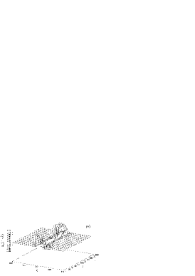
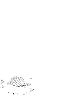
Figure 2: Relaxation dynamics: For a proper illustration of the extension of the radial breather and the forming kink-like angular structure an inner segment of the DNA lattice consisting of $200$ sites is shown. Initial conditions: $d_{\{n_{c}\}}=0.112$ Å. (a) Radial breather.(b) Angular deformation pattern. Development of the kink-like structure.

As becomes evident from Fig. 2–a the vast majority of the excitation energy remains in the initially excited central region and for the radial motion a multi-site breather develops for which the stretching of a base pair distance is larger than the compression characteristic for the evolution in a Morse potential (see also [6]). Moreover, the resulting spatially extended radial breather involves all of the initially excited twenty oscillators evolving with practically equal amplitudes. To either side of the central region the amplitude pattern abruptly goes to zero giving the multi-site breather an almost rectangular spatial profile nearly matching the initial profile. The maintenance of the broad localized radial shape has to be distinguished from the dynamical behavior reported in [7] where, in the context of the BCP model, for similar initial conditions in the radial stretchings in a fairly broad region a merging of the radial components is observed in the course of time which results eventually in a narrow radial pattern localized at a single site only.

For the associated angle deformations $\theta_{n}(t)-\theta_{n}^{(0)}$, emerging from overall initial zero amplitudes, an asymmetric pattern generates rather rapidly in the initially excited region. It holds that the angles from the left (right) of the two central lattice sites (base pairs) decrease (increase) steadily and, the further apart a base pair is from the central ones, the stronger its angular displacement. Eventually, a local kink-like pattern in the angular lattice $\theta_{n}(t)-\theta_{n}^{(0)}$ is created. The horizontal plateaus of the kink-pattern extend continuously in either direction away from the central base pairs so that in the course of time more and more base pairs become subject to angle deformations leading to a progressive untwisting of the central part of the helix [24]. This untwisting of the helicoidal helix structure results from the coupling between the radial and the torsional degrees of freedom due to geometrical constraints and is typical for the DNA opening dynamics [6]. In contrast to the periodically oscillating pattern of the radial variable $d_{n}(t)$, corresponding to alternate stretchings and compressions of the hydrogen bonds, the torsional deformations $\theta_{n}(t)-\theta_{n}^{(0)}$ adjust to a static deformation pattern. For a direct comparison of the extension of the radial to the angular helix deformations, the angular component, expressed in radians, has to be multiplied by $r_{0}\thickapprox 10$ Å  to estimate the associated length scale. We conclude that the degree of the deformations in the angular direction are comparable with those in the radial direction. This has to be distinguished from the observations made for the evolution of narrow radial breathers for which the dynamics of the opening process is dominated by the displacements of the bases in radial direction whose amplitudes are typically larger than those of the angular displacements by at least one order of magnitude [6].

For further illustration of the energy sharing phenomena accompanying the breather formation process, we monitored the time-evolution of the energy contained in the initially excited $20$ base pairs, which is determined by

$$E_{center}(t)=\sum_{\{n_{c}\}}\,\left\{\,\left[\,\sum_{i=1,2}\,E_{kin}(p_{n,i}^{(x)},p_{n,i}^{(y)})+U_{b}(l_{n,\,i})\,\right]+U_{h}(d_{n})\,\right\}.$$ (18)

The temporal behavior of $E_{center}(t)$ is represented by the graph with label $(1)$ in Fig. 6. We observe that in an early phase, lasting for approximately forty time units ($\sim 8\,ps$), a small energy loss takes place and around $1\%$ of the excitation energy flows from the initially excited central region into wider parts of the remainder of the DNA lattice. Afterwards the amplitude of the energy $E_{center}(t)$ fulfills slow oscillations around a mean value. (That this mean value of the energy $E_{center}(t)$ is weakly descending as time progresses indicates further small energy emission from the central region into the rest of the DNA lattice.) The energy emitted from the central region is then mainly redistributed into the angular deformation kink that travels through the DNA lattice in agreement with the formation of the angular pattern represented in Fig. 2–b. Nonetheless, a tiny part of the emission energy is radiated also into the hydrogen bonds outside the central region where it is converted in radial phonons moving uniformly towards the ends of the lattice as just about visible in Fig. 2–a.

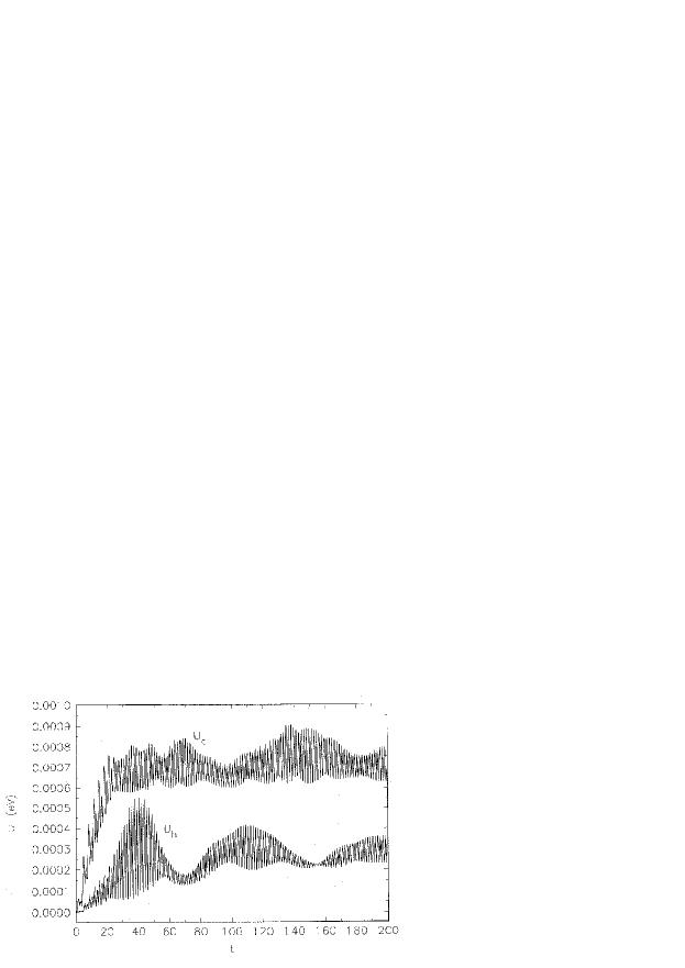
Figure 3: Relaxation dynamics: The distribution of potential energy between the hydrogen bonds and the covalent bonds outside the central region of the DNA lattice.

The Fig. 3 shows the distribution of the energy, between the hydrogen bonds and the covalent bonds, which has been deposited from the central region into the rest of the DNA lattice. Plotted are the time-evolution of the potential energy contained in the displaced hydrogen bonds

$$U_{h}^{c}(t)=\sum_{\tilde{n}}\,(\exp(-d_{n}(t))-1)^{2}\,,$$ (19)

and the potential energy content of the covalent bonds

$$U_{c}^{c}(t)=K\sum_{\tilde{n},\,i=1,2}\,l_{n,i}^{2}(t)\,,$$ (20)

respectively, where $\tilde{n}\in[1,N]\setminus\{n_{c}\}$. After the initial phase of energy absorption a quasi-equilibrium regime is reached and the partial potential energies oscillate around mean values of $0.0007\,eV$ and $0.0003\,eV$ for the deformations of the covalent bonds and the hydrogen bonds, respectively.

Complementary, the energy sharing between the deformed covalent and hydrogen bonds within the initially excited region is illustrated in Fig. 4. During a transient phase of internal energy redistribution the average of the covalent bond energy grows slightly on expense of the hydrogen bond energy. However, the energy migration is not very pronounced. Eventually, the time evolution of each of the two partial potential energies is characterized by periodic oscillations around a (constant) mean value reflecting the attainment of a steady equilibrium regime in the central lattice region. Note that the initial drastic difference in the energy contained in the stretched hydrogen bonds, $U_{h}(0)=0.124\,eV$, and the covalent bonds, $U_{c}(0)=0.018\,eV$, is retained throughout the time-evolution of the respective average partial potential energy.

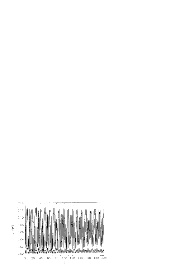
Figure 4: Relaxation dynamics: The energy sharing between the deformed covalent bonds (upper graph) and hydrogen bonds (lower graph) within the initially excited region.

In conclusion, we found that out of an initial non-equilibrium situation, for which the hydrogen bonds in a fairly broad but confined region of the central part of the DNA lattice have been stretched away from their rest lengths, (weak) energy redistribution processes set in, such that small amounts of energy migrate into the remainder of the DNA lattice. During the relaxation process towards an equilibrium of energy balance between the radial and torsional components the angular displacement variables adopt a static kink-like structure. Correspondingly, due to the torsional deformations induced by the opening of the base pairs a local unwinding of the helix develops. Significantly, almost the entire initial excitation energy stays localized in the hydrogen bonds of the central region and a multi-site breather with nearly rectangular profile develops in the radial displacement variables.

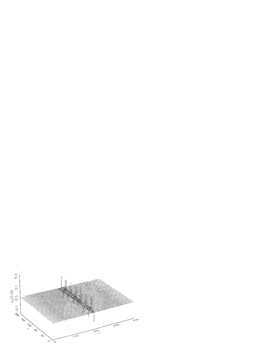
Figure 5: H-bond breather formation for asymmetric initial conditions. Three consecutive sites on one strand possess initially diminished distance to the helix axis.

Besides the initial pattern of broad radial inflation we imposed initially also radial compressions in a fairly broad region of the DNA lattice giving also rise to multi–site breathers corresponding to alternating compressions and stretchings of the H-bonds.

Finally, regarding asymmetric initial conditions we mimicked e.g. the impact of a local ’pushing’ force in cause of which some bases are brought closer to the helix axis. In Fig. 5 we display the spatio-temporal evolution of the radial deformations of the H-bonds when initially three nucleotides at only one strand were displaced from their equilibrium positions. Apparently, even for such asymmetric situations H-bond breathers result characterized by deformations of the hydrogen bonds which are no longer symmetric with respect to the central axis. The conclusion is that the multibreathers are not destroyed by interaction with the modes of the centers of mass . Other numbers of excited base pairs bring about similar results.

4 The relaxation concept and breather construction

We exploit now the findings of the preceding section for the construction of multi-site breathers in DNA. For this goal we initialize the DNA lattice as described above, that is twenty Morse oscillators in the central part of the DNA lattice are elongated from their equilibrium lengths. Subsequently, we let the DNA lattice dynamics relax towards an equilibrium regime during a time interval of $100$ time units. We recall that for such times the energy redistribution between the hydrogen bonds and the covalent bonds and the central region and the remainder of the DNA lattice, respectively has proceeded so far, that virtually negligible alterations of the partial energy contents occur for later times. Notably, a spatially extended radial breather forms on such a time scale. Furthermore, due the geometrical constraint of the helicoidal structure a local untwisting of the double helix arises. The corresponding kink-like pattern in the angle variables encompasses almost the whole lattice, apart from the small parts of the lattice near the boundaries which have not yet experienced angle deformations (cf. Fig. 2–b).

We start now a iteration scheme, for which the quasi-equilibrium solution resulting at the end of the simulation time, viz. the displacements $(x_{n,i}(100)$, $y_{n,i}(100))$, is taken as the new initial condition for the re-iterated DNA lattice dynamics. In order to attain an equilibrium regime of the DNA lattice dynamics the moving radial phonons, carrying the excess energy emitted from the central region, have to be eliminated. In the primary iteration step the radial phonons transport energy merely of the order of $10^{-4}\,eV$. With each further iteration cycle the amount of radial phonon energy, still ejected from the central lattice region, further diminishes. Nevertheless, to accomplish faster relaxation we impose absorbing boundary conditions to the DNA lattice so that the radial phonons are removed, once they arrive at the ends of the lattice. In this iterative manner the energy redistribution from the central region to the remainder of the DNA lattice is more and more reduced and the dynamics relaxes towards a solution of improved energy balance compared to the previous step. To illustrate the latter fact, we display in Fig. 6 the temporal evolution of the energy, $E_{center}(t)$, contained in the central part of the lattice which bears the radial breather. Apparently, convergence of the iteration procedure is achieved already after three iteration steps. In Fig. 7 we depict the resulting radial breather solution. This breather oscillates with a period of $=0.7\,ps$ which is a realistic value for the time scale of experimentally observed vibrational modes occurring prior to the opening process in DNA melting [25]. More importantly, the broad localized radial excitation pattern comprises twenty base pairs and the maximal elongation of a base pair radius from rest length is about $0.122$ Å . Thus, we are able to create long-lived spatially extended radial breathers of fairly large amplitude in DNA representing the oscillating ’bubbles’ as the precursor to thermal denaturation. Finally, we remark that, depending on the choice of the width of the initial excitation pattern, with our relaxation-method radial DNA breathers of varying extension can be generated. These breathers range up from narrow ones (effectively one-site) up to very broad breathers involving up to even fifty lattice sites. As the choice of the initial excitation pattern is further concerned, we tried, besides the radial rectangular profiles, also other profiles such as bell-shaped ones given by $d_{\{n_{c}\}}(0)=A_{0}/\cosh[\beta\,(n-n_{0})]$. $A_{0}$, $\beta$ and $n_{0}$ are constants fixing the amplitude, the spatial extension and the center of the starting profile, respectively. In the outcome of the relaxation dynamics we observed bell-shaped radial breathers nearly preserving the initial profile analogous to the results reported earlier in this manuscript for the broad breathers. The same holds when additionally to the radial displacements also initial kink-like twist deformations are considered.

Figure 6: Breather construction: The temporal evolution of the energy contained in the central part of the lattice for the first, the second and the third step of the iteration procedure, respectively, as indicated in the plot. The energies are normalized in units of the initial energy of the first iteration $E_{center}(0)$.

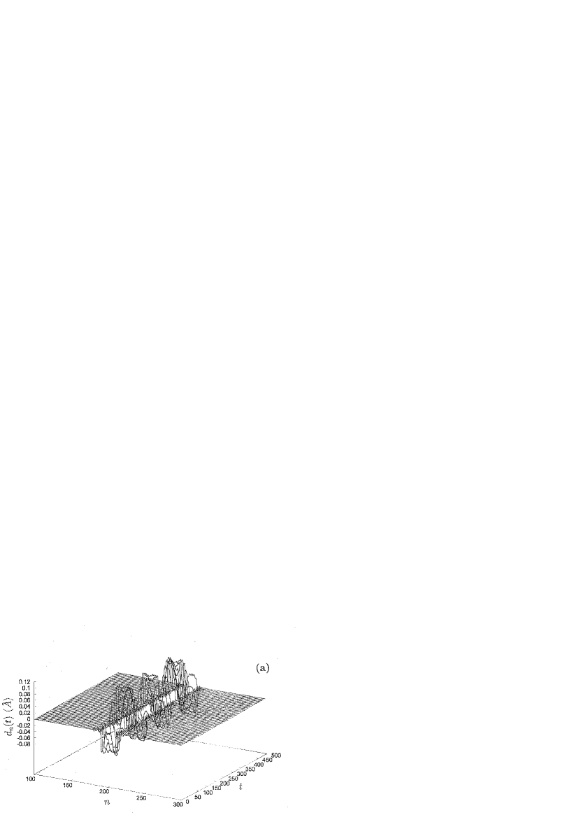
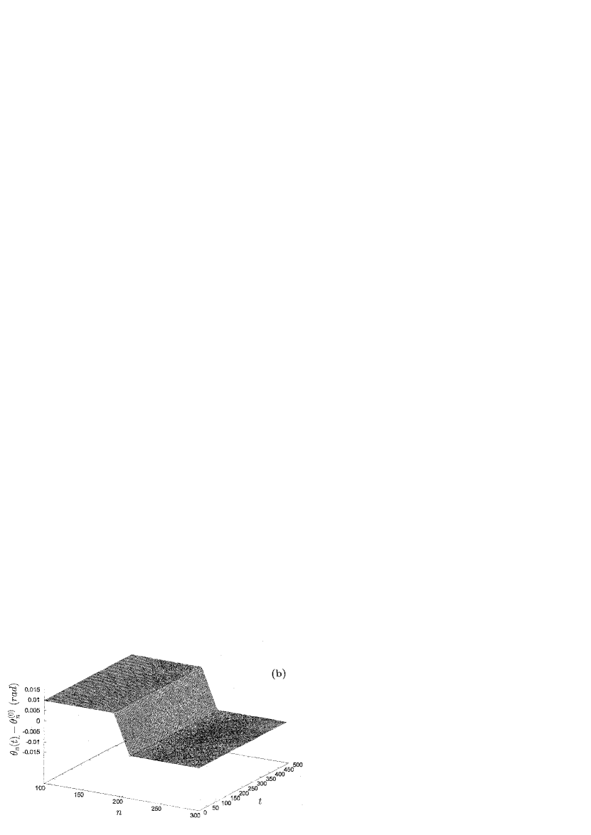
Figure 7: Breather construction: The final radial breather solution obtained after three iteration steps of the relaxation concept.

For a more elaborate study of nonlinear vibrational modes in DNA the effects of external influences have to be included. Real DNA molecules exhibit random structural imperfections of their double helix caused, e.g., by the deforming impact of the chemical surroundings when DNA gets buffeted by water molecules. Another source for structural irregularities originates from the random base sequence of the genetic code. In addition, the varying hydrophobic potential of the base pair interactions depending on the ambient aqueous solvent may leave the helix structure in an irregularly distorted shape. Accordingly, for an improvement of our model, irregularity effects can be mimicked by taking into account structural disorder so that the resulting irregular helical DNA matrix deviates from the perfectly regular helix structure. (The formerly discussed ordered, regular structure arises, for example, for synthetically produced DNA molecules consisting of a single type of base pairs, for instance, poly(G)-poly(C) DNA polymers, surrounded by vacuum.)

To be precise, we consider randomly distributed equilibrium coordinates, $\tilde{x}_{n,i}^{(0)}$ and $\tilde{y}_{n,i}^{(0)}$, of the bases with $\tilde{x}_{n,i}^{(0)}-x_{n,i}^{(0)}\in[-\Delta x_{n,i},\Delta x_{n,i}]$ and $\tilde{y}_{n,i}^{(0)}-y_{n,i}^{(0)}\in[-\Delta y_{n,i},\Delta y_{n,i}]$. The intervals of the deviations $\Delta x$ and $\Delta y$ range up to $5\%$ of the respective rest value $x_{n,i}^{(0)}$ and $y_{n,i}^{(0)}$ of the corresponding regular structure.

In Fig. 8 we show a representative case for the DNA lattice dynamics for one realization of structural disorder. In addition to the disordered helicoidal structure also random amplitudes of the initial values for the distance displacements, $d_{\{n\}}(0)$, in the central region have been chosen. Apparently, the H-bridge breather is robust sustaining the influence of disorder and virtually resembles the behavior of the ordered case (compare Fig. 2–a).

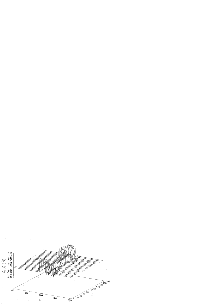
Figure 8: Breather construction: The persisting radial breather for a disordered helicoidal equilibrium structure (see text). The initial values for the irregular distance displacements in the central region, $\tilde{d}_{\{n_{c}\}}$, are randomly distributed according to $\tilde{d}_{\{n_{c}\}}-d_{\{n_{c}\}}\in[-\Delta d,\Delta d]$. The interval of the deviations $\Delta d$ ranges up to $5\%$ of the respective value $d_{\{n_{c}\}}$ of the regular case depicted in Fig. 2.

On the other hand, when the amount of excitation energy placed in the central lattice sites, exceeds a critical value, $E_{n_{c}}\gtrsim 0.6\,eV$, or equivalently when the hydrogen bonds get elongated too far, we do not longer observe the relaxation towards a stable multi-site radial breather as in the previous (lower-energy) cases. Instead directed flow of energy into one of the initially excited lattice sites takes place related with the simultaneous energy depletion of the remaining lattice sites. In this manner, the transferred energy is accumulated in the corresponding hydrogen bond of the energy-gaining site with the result that the radial elongation continually grows. Eventually, the corresponding hydrogen bridge is stretched so far that it breaks up. This energy concentration onto a single site and the succeeding bond breaking process is illustrated in Fig. 9.

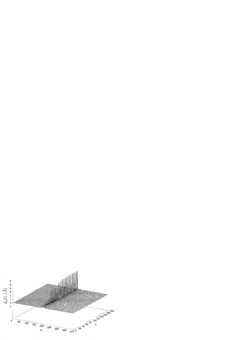
Figure 9: Concentration of the excitation energy on a single site of the DNA lattice and successive bond breaking. Initial conditions corresponding $d_{\{n_{c}\}}=0.75$ AA corresponding to an amount of excitation energy of $0.646\,eV$.

Conversely, even for as tiny radial displacement amplitudes as $d_{\{n\}}(0)\sim 10^{-5}$ Å, corresponding to a lattice excitation energy of the order of $10^{-7}\,eV$, the energy stays localized at the twenty initially lattice sites and a radial multi-site breather is formed. This demonstrates impressively that DNA possesses very efficient energy storing abilities. It should be mentioned, that usually, in studies of nonlinear oscillator networks one observes that for undercritical amplitudes, being tantamount to a low degree of inherent nonlinearity, an initially localized structure decays rather rapidly and the excitation energy gets uniformly distributed over the whole lattice [26].

It should be noted that Campa [11] also shows the existence of broad bubbles that move along the molecule. The differences between his model and ours are commented in the previous section. The results are quite different. The Campa bubbles have no oscillation and a bell profile, while our multibreathers oscillate and have a quasi rectangular profile, involving a larger number of base pairs in a similar way. The oscillation is a major weakness of our bubbles as they can only be considered as precursors of transcription or denaturation. They have some advantage, however, which are their quasi homogenous amplitude and that they are more generic, being the consequence of the helical shape, and not relying on evolving in the flat part of the Morse potential.

5 Linear modes

In this section we consider the linear modes of the system and their influence on the behavior and stability of the system. The linear equations corresponding to Eqs. (12–15) for the homogeneous and symmetric system are given by:

$$\ddot{x}_{n,i}=(-1)^{i}\,2\left(d_{n}^{x}\,\Delta x_{n}+d_{n}^{y}\,\Delta y\right)\frac{d_{n}^{x}}{d_{0}^{2}}$$ (21)

$$-2\,K(\frac{L_{n,i}^{x}}{l_{0}^{2}}[L_{n,i}^{x}\delta x_{n,i}+L_{n,i}^{y}\delta y_{n,i}]-\frac{L_{n+1,i}^{x}}{l_{0}^{2}}[L_{n+1,i}^{x}\delta x_{n+1,i}+L_{n+1,i}^{y}\delta y_{n+1,i}]\,)\,,$$

$$\ddot{y}_{n,i}=(-1)^{i}\,2\left(d_{n}^{x}\,\Delta x_{n}+d_{n}^{y}\,\Delta y\right)\frac{d_{n}^{y}}{d_{0}^{2}}\,,$$ (22)

$$-2\,K(\frac{L_{n,i}^{y}}{l_{0}^{2}}[L_{n,i}^{x}\delta x_{n,i}+L_{n,i}^{y}\delta y_{n,i}]-\frac{L_{n+1,i}^{y}}{l_{0}^{2}}[L_{n+1,i}^{x}\delta x_{n+1,i}+L_{n+1,i}^{y}\delta y_{n+1,i}]\,)$$

where $\Delta x_{n}=x_{n,1}-x_{n,2}$, $\Delta y_{n}=y_{n,1}-y_{n,2}$, $\delta x_{n}=x_{n,i}-x_{n-1,i}$ and $\delta y_{n}=y_{n,i}-y_{n-1,i}$. In the symmetric equilibrium state it holds that $L_{n,2}^{x}=-L_{n,1}^{x}=L_{0}\cos(\phi_{n}^{(0)})$, $L_{n,2}^{y}=-L_{n,1}^{y}=L_{0}\sin(\phi_{n}^{(0)})$, $d_{n,x}=d_{0}\,\cos(\theta_{n}^{(0)})$, $d_{n,y}=d_{0}\,\sin{\theta_{n}^{(0)}}$, with $L_{0}=((L_{n}^{x})^{2}+(L_{n}^{y})^{2})^{1/2}=d_{0}\sin(\theta_{0}/2)$, being the equilibrium horizontal distance between nucleotides along one strand; $\phi_{n}^{(0)}$ being the angular cylindrical coordinate of the vector that goes from nucleotide $n-1$ to $n$ along strand $1$ at equilibrium, i.e., $\phi_{n}^{(0)}=\theta_{n}^{(0)}-\theta_{0}/2+\pi/2$; and $\theta_{n}^{(0)}=n\,\theta_{0}$, as defined in Eq. 3, at equilibrium.

The natural coordinate system for each base pair is given by the projections on the unit vectors $\mathbf{e}_{r}=(\cos(\theta_{n}^{(0)}),\sin(\theta_{n}^{(0)}),0)$ and $\mathbf{e}_{\theta}=(-\sin(\theta_{n}^{(0)}),\cos(\theta_{n}^{(0)}),0)$, and the natural variables are the relative displacements of the base pairs $\Delta\mathbf{r}_{n}=(\Delta x_{n},\Delta y_{n},0)=(x_{n,1}-x_{n,2},y_{n,1}-y_{n,2},0)$, and the positions of their centers of mass in the horizontal plane: $\overline{\mathbf{r}}_{n}=(\overline{x}_{n},\overline{y}_{n},0)=((x_{n,1}+x_{n,2})/2,(y_{n,1}+y_{n,2})/2,0)$. Therefore, the natural coordinates are:

$$r_{n} = \Delta\mathbf{r}_{n}\cdot\mathbf{e}_{r}=\cos(\theta_{n}^{(0)})\Delta x_{n}+\sin(\theta_{n}^{(0)})\Delta y_{n}\,,$$

$$\alpha_{n} = \frac{\Delta\mathbf{r}_{n}\cdot\mathbf{e}_{\theta}}{d_{0}}=\frac{1}{d_{0}}\left(-\sin(\theta_{n}^{(0)})\Delta x_{n}+\cos(\theta_{n}^{(0)})\Delta y_{n}\right)\,,$$

$$\overline{r}_{n} = \overline{\mathbf{r}}_{n}\cdot\mathbf{e}_{r}=\cos(\theta_{n}^{(0)})\overline{x}_{n}+\sin(\theta_{n}^{(0)})\overline{y}_{n}\,,$$

$$\overline{s}_{n} = \overline{\mathbf{r}}_{n}\cdot\mathbf{e}_{\theta}=-\sin(\theta_{n}^{(0)})\overline{x}_{n}+\cos(\theta_{n}^{(0)})\overline{y}_{n}\,.$$ (23)

To first order in the perturbations $\{x_{n,i}\}$,$\{y_{n,i}\}$, $r_{n}\simeq d_{n}$ represent the stretchings of the base pairs; $\alpha_{n}\simeq\arctan[(d_{n}^{y}+\Delta y_{n})/(d_{n}^{x}+\Delta x_{n})]-\theta_{n}^{(0)}(\mathrm{mod}\,\pi)$, the relative twist angle with respect to the equilibrium position. $\overline{r}_{n}$ and $\overline{s}_{n}$ are the displacements of the base pairs centers of mass in the directions of the bonds or orthogonal to them respectively. In terms of these variables, the linear dynamical equations (21–22) can be written as:

$$\ddot{\overline{r}}_{n} = -\mu\,\sin^{2}(\frac{\theta_{0}}{2})\,(2\,\overline{r}_{n}+\overline{r}_{n+1}+\overline{r}_{n-1})-\mu\,\sin(\frac{\theta_{0}}{2})\cos(\frac{\theta_{0}}{2})\,(\overline{s}_{n+1}-\overline{s}_{n-1})\,,$$

$$\ddot{\overline{s}}_{n} = \mu\,\sin(\frac{\theta_{0}}{2})\cos(\frac{\theta_{0}}{2})\,(\overline{r}_{n+1}-\overline{r}_{n-1})-\mu\,\cos^{2}(\frac{\theta_{0}}{2})\,(2\,\overline{s}_{n}-\overline{s}_{n+1}-\overline{s}_{n-1})\,,$$

$$\ddot{r}_{n} = -\omega_{0}^{2}\,r_{n}$$

$$- \mu\,\sin^{2}(\frac{\theta_{0}}{2})\,(2\,r_{n}+r_{n+1}+r_{n-1})-\mu\,\sin(\frac{\theta_{0}}{2})\cos(\frac{\theta_{0}}{2})\,d_{0}\,(\alpha_{n+1}-\alpha_{n-1})\,,$$

$$d_{0}\,\ddot{\alpha}_{n} = \mu\,\sin(\frac{\theta_{0}}{2})\cos(\frac{\theta_{0}}{2})\,(r_{n+1}-r_{n-1})-\mu\,\cos^{2}(\frac{\theta_{0}}{2})\,d_{0}\,(2\,\alpha_{n}-\alpha_{n+1}-\alpha_{n-1})\,,$$

with $\mu=2\,K\,(L_{0}/l_{0})^{2}$.

The first two equations describe the motion of the helix as a whole, their corresponding linear modes frequencies will be referred to as the cm (center of mass) branch. The last two equations represent the dynamics of the base pairs and lead to two branches, referred to as the bp (base pair) acoustic and optical branches. Note that the cm equations are independent of the bp equations and so are their modes.

The frequencies of the cm branch are given by:

$$\omega^{2}=2\mu\,[\,1-cos(\theta_{0})cos(q)]\,,$$ (25)

and a branch of zeros, which represents the possible motions of the helix to other equilibrium positions.

The bp branches are:

$$\omega^{2}_{\pm} = \frac{1}{2}\left(\omega_{0}^{2}+2\,\mu\,[1-\cos(\theta_{0})\cos(q)]\right)$$ (26)

$$\pm \frac{1}{2}\sqrt{\left(\omega_{0}^{2}+2\,\mu\,[1-\cos(\theta_{0})\cos(q)]\right)^{2}-8\,\mu\,\omega_{0}^{2}\cos^{2}(\theta_{0}/2)\sin^{2}(q/2)}\,.\quad$$

The sign $+$ and $-$ correspond to the bp optical and acoustic branches respectively.

Fig. 10–a shows the dependance of the phonon spectrum on the coupling parameter $K$ and Fig. 10–b depicts the three branches for the value of $K=0.683$ used in this article. It can be seen that there is a phonon gap for values of $K<K_{c}$ with $K_{c}\simeq 0.7$. The Fourier spectrum of the multi-breathers found consists of a single frequency $\omega_{b}$ slightly below $\omega_{0}=2$, the frequency of the isolatedly vibrating base pairs, and its harmonics. Furthermore, the modes in the neighborhood of $\omega_{b}$ have wave vector $q=\pi$ and therefore they are not much excited by the perturbation of the radial variables.

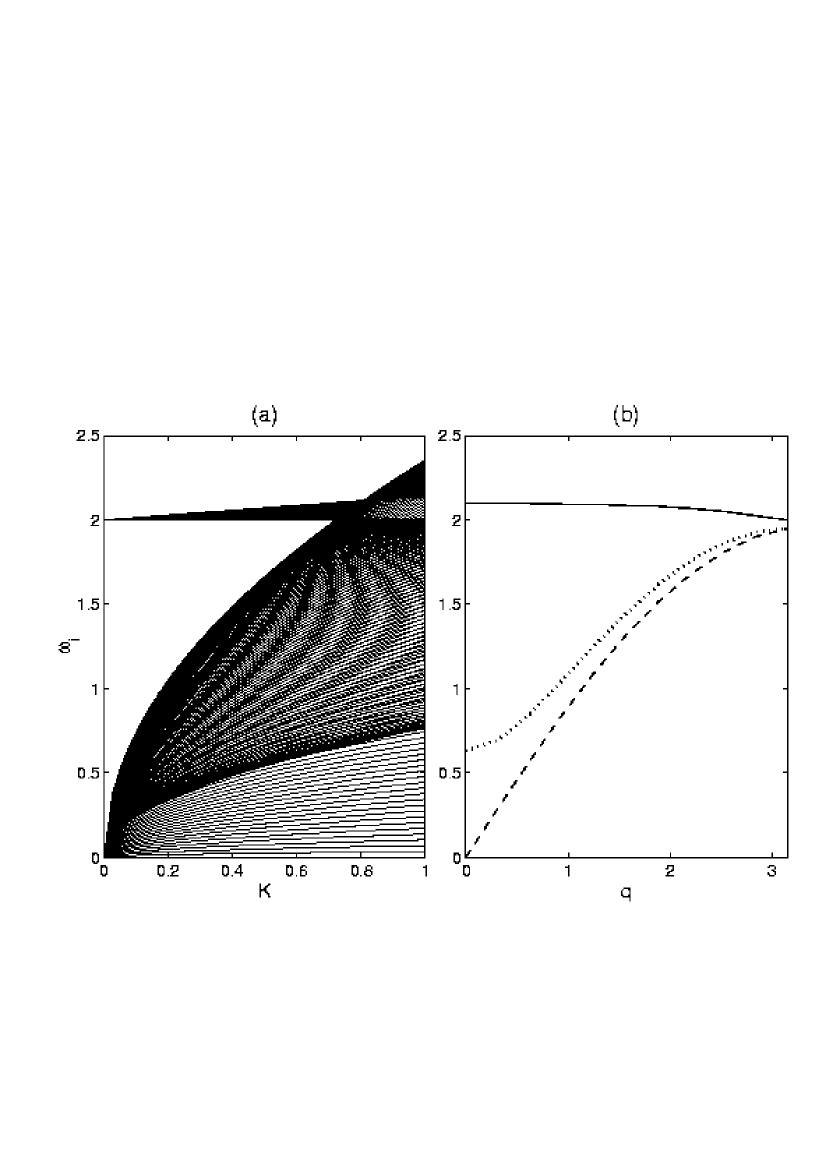
Figure 10: Spectral analysis of the linear system. (a) Dependence of the phonon spectrum on the longitudinal elastic constant $K$. For values of $K$ below $K_{c}\simeq 0.7$ there exist a gap below the optical branch where the frequencies of the multi-site breathers lie. (b) Frequencies of the three phonon branches with respect to their wave numbers $q$. The $\pi$ modes are the ones on the vicinity of the multi-site breather frequency.

A remarkable fact of the phonon spectrum for $K<K_{c}$ is the inversion of the optical spectrum with respect to the planar PB model [2]. In the latter, the only variables are the distances between bases within each base pair, and the coupling proposed is a standard attractive one, which has been made more complex afterwards [27, 28], but without consequences on the phonon spectrum. The dynamical equations are given by:

$$\ddot{u}_{n}+V^{\prime}(u_{n})+\epsilon\,(2\,u_{n}-u_{n-1}-u_{n+1})=0\,,$$ (27)

being $V$ the Morse potential with $V^{\prime\prime}(0)=\omega_{0}^{2}>0$ and $\epsilon>0$. The dispersion relation is given by $\omega^{2}=\omega_{0}^{2}+4\epsilon\sin^{2}(q/2)$. There are some consequences for this system [29, 30]: a) the bottom (linear) mode has $q=0$, and the top one has $q=\pi$; b) one–site breathers are stable; c) the tails of a breather or multibreather consists of in–phase oscillators; d) multibreathers with all the oscillators in phase (derived from $q=0$) are unstable and with all the oscillators out of phase (derived from $q=\pi$) are stable [31, 33, 34, 35]. If the value of $\epsilon$ were negative, the conclusions would be reversed.

In the model proposed in this article considering the helical shape of the DNA molecule, the optical spectrum is inverted as can be seen in Eqs. LABEL:eq:lincmbp. Due to the degeneracies of the model we have not been able to obtain exact breathers, but the Fourier spectrum just shows a frequency below the optical branch and its harmonics, which means that they are standard breathers in the usual meaning, i.e., localized, nonlinear, periodic oscillations. The tails of the multibreathers are, indeed, of the $q=\pi$ type, according to this inversion. However, the transcendental consequence arising from the inversion of the effective type of coupling is that the multibreathers are stable. This is a result that should not be overlooked: the helical shape of the DNA molecule provides a means for stable, large amplitude oscillations of base pairs groups, i.e, for the formation of the denaturation bubble.

6 Summary

In the present work we have studied the formation process of broad H-bridge breathers in DNA molecules. The double helix formation of DNA has been described in terms of an oscillator model relying on the base-pair picture. In this context each base pair possesses four degrees of freedom, namely a radial, an angular one, and two motions for the base pairs centers of mass. For an extension of the BCP model [6] we have treated the two strands individually allowing for asymmetric vibrations of the H-bridges. As for the simplifications of our DNA model, we remark that we have not distinguished between the four different base types and therefore, have treated each base as a single entity of fixed mass. Apart from this, we neglected also the different types of hydrogen bonds between the two different pairings in DNA, namely the bridging of the G-C and the A-T pairs by three and two hydrogen bonds, respectively.

We concentrate in this paper on the effect of the helical shape of the DNA molecule, avoiding the introduction of other potential terms to make it apparent. The result is that this shape brings about a inversion of the effective type of coupling, with a inversion of the phonon spectrum, that allows for the existence of stable multi–site breathers.

We have demonstrated that in the course of the relaxation dynamics of DNA molecules, which have been displaced in a certain region from their equilibrium configuration, an equilibrium state is attained. More precisely, starting from a radially distorted configuration involving several consecutive base pairs the twist-opening dynamics relaxes towards a localized state. The latter is built up from a multi-site H-bridge breather in combination with a static kink-like profile of the angular variables connected with the untwist of the helix. Excess energy, not to be contained in the radial breather, is emitted from the initially excited region in the form of radial phonons approaching either ends of the DNA lattice. The relaxation process and the attainment of a stable breather regime has also been observed for asymmetric initial conditions when e.g. bases on only one of the two strands are displaced from their equilibrium positions.

We have exploited then the dynamical approach of an equilibrium state for the construction of breather states of the DNA. To this aim we have established an iteration scheme, such that, with increasing steps of applied iterations the dynamics gets closer to an equilibrium regime supporting a radial breather together with a kink-like pattern in the angular components. It should be stressed that the obtained broad H-bridge breathers reproduce realistically the extension of the oscillating bubbles observed in DNA. However, the almost rectangular shape of our H-bridge breather solution has to be distinguished from the single-site radial breather being reminiscent of an envelope soliton solution with a half-width of twenty base pairs obtained in the context of the BCP model in Ref.  [7]. The multi-site breather with all of its constituents performing in-phase oscillations of equal amplitude renders all of the involved base pairs accessible to the functional process (e.g. the transcription) on an equal footing in contrast to the uneven and less efficient separation of the two strands associated with the bell- shaped amplitude pattern when the breather is centered at a single site so that merely the half width of the exponentially localized profile comprises $15-20$ base pairs.

Our iteration scheme for the construction of H-bridge breathers is applicable so long as the amplitudes of the radial distortions do not exceed a critical value. However, for overcritically large amplitude (or equivalently, too large amount of excitation energy) the dynamics does no longer relax onto a broad H-bridge breather. Remarkably, one rather observes the directed flow of excitation energy in a single H-bond with the consequence that this bond may even break up.

Finally, we note that with view to the role of structural disorder, we have found that the broad H-bond breathers sustain moderate amount of randomness in the arrangement of the equilibrium positions of the bases as well as in the initial local displacement patterns.

Acknowledgments

One of the authors (D.H.) acknowledges support by the Deutsche Forschungsgemeinschaft via a Heisenberg fellowship (He 3049/1-1). J.F.R.A acknowledges partial support under the LOCNET EU network HPRN-CT-1999-00163 and D.H. and the Institut für Theoretische Physik for their warm hospitality

References

- [1] L. Stryer Biochemistry, Freeman, New York (1995).
- [2] M. Peyrard and A.R. Bishop, Phys. Rev. Lett. 62, 2755 (1989).
- [3] L.V. Yakushevich, Quart. Rev. Biophys. 26, 201 (1993).
- [4] G. Gaeta, C. Reiss, M. Peyrard and T. Dauxois, Riv. Nuovo Cim. 17, 1 (1994).
- [5] M. Barbi, Localized Solutions in a Model of DNA Helicoidal Structure, PhD Thesis, Universit degli Studi di Firenze (1998).
- [6] M. Barbi, S. Cocco and M. Peyrard, Phys. Lett. A 253, 358 (1999).
- [7] M. Barbi, S. Cocco, M. Peyrard and S. Ruffo, J. Biol. Phys. 24, 97 (1999).
- [8] S. Cocco and R. Monasson, Phys.Rev. Lett. 83(24), 5178 (1999).
- [9] S. Cocco and R. Monasson, J. Chem. Phys. 112, 10017 (2000).
- [10] J. Agarwal and D. Hennig, Physica A. To appear. (2000).
- [11] A. Campa, Phys. Rev. E 63, 021901 (2001). To appear. (2000).
- [12] T. Lipniacky, Phys. Rev. E 64, 051919 (2001).
- [13] J.L. Marín and S. Aubry, Nonlinearity 7, 1623 (1996).
- [14] T. Dauxois, M. Peyrard and A.R. Bishop, Phys. Rev. E 47, 684 (1993).
- [15] S.L. Nyeo and I.C. Yang, Mod. Phys. Lett. 14, 313 (2000).
- [16] N. Theodorakopoulos, T. Dauxois and M. Peyrard, Phys. Rev. Lett. 85, 6 (2000).
- [17] J.F. Marko and E.D. Siggia, Science 265, 506 (1994); T.R. Strick, J.F. Allemand, D. Bensimon, A. Bensimon, and V. Croquette, Science 271, 1835 (1996).
- [18] S.B. Smith, L. Finzi and C. Bustamante, Science 258, 1122 (1992).
- [19] B. Essevaz-Roulet, U. Bockelmann and F. Heslot, Proc. Natl. Acad. Sci. U.S.A. 94, 11935 (1197).
- [20] U. Bockelmann, B. Essevaz-Roulet, and F. Heslot, Phys. Rev. Lett. 79, 4489 (1997); Phys. Rev. E 58, 2386 (1998).
- [21] H. Clausen-Schaumann, M. Rief, C. Tolksdorf, H.E. Gaub, Biophys. J. 78, 1997 (2000).
- [22] N.J. Crisona, T.R. Strick, D. Bensimon, V. Croquette and N.R. Cozzarelli, Genes Dev. 14, 2881 (2000).
- [23] Y.-J. Ye, R.-S. Chen, A. Martinez, P. Otto and J. Ladik, Sol. Stat. Comm. 112, 139 (1999).
- [24] J.D. Moroz and P. Nelson, Proc. Natl. Acad. Sci. U.S.A. 94, 14418 (1997).
- [25] E.W. Prohofsky, K.C. Lu, L.L van Zandt and B.F. Putnam, Phys. Lett. A 70, 492 (1979).
- [26] S. Flach and C.R. Willis, Physics Reports 295, 181 (1998).
- [27] T. Dauxois, M. Peyrard and A.R. Bishop, Phys. Rev. E 47(1), R44 (1993).
- [28] Y. Zhang, W. Zheng, J. Liu and Y. Z. Chen, Phys. Rev. E 56(6), 7100 (1997).
- [29] J.L. Marín and S. Aubry, Nonlinearity 9, 1501 (1996).
- [30] J.L. Marín, S. Aubry and LM Floría, Physica D 113, 283 (1998).
- [31] J.L. Marín, Ph. D. dissertation, Universidad de Zaragoza, 1997.
- [32] S. Aubry, Physica D 103, 201 (1997).
- [33] A.M. Morgante, M. Johansson, G. Kopidakis and S. Aubry, Physica D 162, 53 (2002).
- [34] A. Alvarez, J.F.R. Archilla, J. Cuevas and F.R. Romero, New Journal of Physics 4, 72.1 (2002).
- [35] J.F.R. Archilla, J. Cuevas, B. Sánchez–Rey and A. Alvarez, Physica D 180, 235 (2003).