Classical Resonances and Quantum Scarring

Abstract

We study the correspondence between phase-space localization of quantum (quasi-)energy eigenstates and classical correlation decay, given by Ruelle-Pollicott resonances of the Frobenius-Perron operator. It will be shown that scarred (quasi-)energy eigenstates are correlated: Pairs of eigenstates strongly overlap in phase space (scar in same phase-space regions) if the difference of their eigenenergies is close to the phase of a leading classical resonance. Phase-space localization of quantum states will be measured by $L^{2}$ norms of their Husimi functions.

1 Introduction

Schnirelman’s theorem [1] as well as Berry’s physical reasoning predict that quantum energy eigenfunctions (Wigner or Husimi representation [2, 3]) of systems whose classical counterpart is chaotic are uniformly distributed on the energy shell. Heller, however, has shown that there exist quantum eigenfunctions which are strongly localized (scarred) on hyperbolic periodic orbits [4]. At present, the general opinion is that scars are exceptional, while the majority consits of uniformly (phase-space) distributed eigenstates [5]. On the other hand, it is well known that there also exist weakly localized eigenfunctions, which continuously fill the “gap” between uniformly distributed and strongly localized eigenfunctions. Conveniently, instead of single exceptions we here consider localization properties of the whole set of eigenfunctions of the system; restricting our studies on finite dimensional Hilbert spaces. To that purpose, we introduce squared $L^{2}$ norms of Husimi eigenfunctions as a measure for phase-space localization [6]. As it will be shown in the sequel this measure proves amenable to semiclassical considerations.

The classical dynamics of chaotic systems can be described by the time evolution of phase-space density functions. The corresponding propagator is the Frobenius-Perron operator [7, 8, 9], where the poles of its resolvent are called Ruelle-Pollicott resonances which coincide with decay rates of classical correlation functions [10, 11, 12, 13]. The quantum-classical correspondence, in particular the influence of Ruelle-Pollicott resonances on the quantum energy spectrum, is still a point of interest [14, 15, 16, 17]. We show that phase-space overlaps of energy eigenstates turn out Lorentz distributed with respect to the differences of their eigenenergies. The Lorentzians are determined by Ruelle-Pollicott resonances. In other words, the probability that two eigenstates strongly overlap becomes large if the difference of their eigenenergies coincides with the position where the Lorentzian is peaked. On the other hand, if a pair of eigenstates strongly overlaps (much more than random-matrix theory predicts) each of them must be localized, i.e. scarred, in the same phase-space regions.

We here consider systems with a compact two-dimensional phase space, in particular the unit sphere, whereby the Hilbert-space dimension of the quantum counterpart becomes finite. Periodically driving destroyes integrability in general. Moreover, a stroboscopic description leads to a Hamilton map or a Floquet operator in the classical or quantum case, respectively. A well known representative of such a dynamics is the kicked top [18, 19, 20].

2 Kicked Top

The dynamics of the kicked top is described by a stroboscopic map of an angular momentum vector whose length is conserved, For such a dynamics the phase spaces is the unit sphere. The classical time evolution is usually described in the “Hamilton picture”, whereby the stroboscopic consideration leads to a Hamilton map which describes a trajectory after each period,

$$(q^{\prime},p^{\prime})={\cal M}(q,p)\,.$$ (1)

Here the primes denote the final position $q$ and momentum $p$ coordinates. On the sphere the canonical phase-space coordinates are given by the azimuthal and polar angle as $q=\varphi$ and $p=\cos\theta$.

The quantum time evolution in the Schrödinger picture is generated by a Floquet operator $F$ which is built by the components of an angular momentum operator ${\bf J}$; we choose it as a sequence of rotations about the $y$ and $z$-axis followed by a nonlinear torsion about the $z$-axis,

$$F = T_{z}(\tau)R_{z}(\alpha)R_{y}(\beta)\,,$$ (2)

$$T_{z}(\tau)={\rm e}^{-{\rm i}\frac{\tau}{N}J_{z}^{2}}\,,$$

$$R_{z}(\alpha)={\rm e}^{-{\rm i}\alpha J_{z}}\,,$$

$$R_{y}(\beta)={\rm e}^{-{\rm i}\beta J_{y}}\,,$$

where $\tau$ is called the torsion strength and $\alpha$ and $\beta$ are rotation angles. The dimension of the quantum Hilbert space is $N=2j+1$, where $j$ is the quantum angular momentum formally replacing the inverse of Planck’s constant, $\hbar^{-1}$ ($\hbar=1$ in this article). Since $F$ is unitary, it has $N$ orthogonal eigenstates with unimodular eigenvalues characterized by eigenphases (quasi-eigenenergies) as $F^{n}|\phi_{i}\rangle=\exp(-{\rm i}n\phi_{i})|\phi_{i}\rangle$.

The classical counterpart has in general a mixed phase space. By the choice of the parameters as $\alpha=\beta=1$ and $\tau=10$ the dynamics becomes strongly chaotic. For $j=200$ which we use for numerical results stable island are not resolved by the Planck cell of size $\frac{4\pi}{N}$, whereby the dynamics looks, from a quantum point of view, effectively hyperbolic.

In order to compare the results of the kicked top with those of random-matrix theory (RMT) we here discuss the symmetries of the system. The dynamics proves invariant under nonconventional time reversal. In terms of random-matrix theory the Floquet matrix belongs to the circular orthogonal ensemble (COE), where the coefficients of the eigenvectors can be chosen real in a suitable basis [21, 22]. We here expand the Floquet operator in the basis of eigenstates of the $z$-component of the angular momentum operator, $J_{z}|jm\rangle=m|jm\rangle$. By a unitary transformation given by a simple rotation, $F^{\prime}=\tilde{R}F\tilde{R}^{\dagger}$, the Floquet matrix becomes symmetric, ${F^{\prime}}^{T}=F^{\prime}$, where the eigenvectors become real. Here $T$ denotes transposition. This is an important property, since the $L^{2}$ norm of a Husimi function which we will use as a measure for phase-space localization is invariant under rotations. Therefore, eigenvectors of the kicked top must be compared to real random vectors. The rotation is of form $\tilde{R}=R_{z}(\frac{{}_{\beta}}{{}^{2}})R_{y}(-\frac{{}_{\pi}}{{}^{2}})R_{z}(-\frac{{}_{\pi}}{{}^{2}})$, whereby the transformed Floquet matrix becomes

$$F^{\prime}=R_{z}(\frac{{}_{\beta}}{{}^{2}})R_{y}(-\frac{{}_{\pi}}{{}^{2}})R_{z}(-\frac{{}_{\pi}}{{}^{2}})T_{z}(\tau)R_{z}(\alpha)R_{y}(\beta)R_{z}(\frac{{}_{\pi}}{{}^{2}})R_{y}(\frac{{}_{\pi}}{{}^{2}})R_{z}(-\frac{{}_{\beta}}{{}^{2}})\,.$$ (3)

After commutation of the rotation $R_{z}(-\frac{{}_{\pi}}{{}^{2}})$ with the torsion the product

$$R_{z}(-\frac{{}_{\pi}}{{}^{2}})R_{y}(\beta)R_{z}(\frac{{}_{\pi}}{{}^{2}})=R_{y}(\frac{{}_{\pi}}{{}^{2}})R_{z}(\beta)R_{y}(-\frac{{}_{\pi}}{{}^{2}})$$ (4)

is a rotation about the $x$-axis. Using the latter relation the transformed Floquet matrix finally becomes

$$F^{\prime}=\Big{(}R_{y}(\frac{{}_{\pi}}{{}^{2}})R_{z}(\frac{{}_{\beta}}{{}^{2}})\Big{)}^{T}T_{z}(\tau)R_{z}(\alpha)R_{y}(\frac{{}_{\pi}}{{}^{2}})R_{z}(\frac{{}_{\beta}}{{}^{2}})\,,$$ (5)

which is obviously symmetric.

3 Frobenius-Perron Operator

Another way to describe classical time evolution is the “Liouville picture”, as the propagation of density in phase space. The corresponding propagator, the Frobenius-Perron operator ${\cal P}$, is defined through the Hamilton map as

$$f_{n}(q,p)={\cal P}f_{0}(q,p)=f_{0}({\cal M}^{-n}(q,p))=\int{\rm d}q^{\prime}\,{\rm d}p^{\prime}\,f_{0}(q^{\prime},p^{\prime})\delta^{2}((q^{\prime},p^{\prime})-{\cal M}^{-n}(q,p))\,,$$ (6)

where $f(q,p)$ denotes an arbitrary phase-space density function. Note that the Hamilton map is invertible and area preserving. An expectation value of a classical observable is given by the phase-space integral

$$\left\langle A\right\rangle=\int{\rm d}q\,{\rm d}p\,A(q,p)f(q,p)\equiv\mbox{\bf(}A\mbox{$|\!\!|$}f\mbox{\bf)}\,,$$ (7)

where we have introduced the Dirac notation. To avoid confusion with quantum wave functions we here use round brackets. Note that this notation is generally to read as a linear functional, where the density function $f$ belongs to the Banach space $L^{1}$ and the observable $A$ to the dual space $L^{\infty}$. Furthermore, we suppose that both functions are real, otherwise $A$ is to complex conjugate in the integral notation (7).

For classically chaotic systems (we assume purely hyperbolic dynamics) correlations of observables decay exponentially in time. Due to ergodicity the time correlation can be written by a phase-space integral,

$$C_{AB}(n)=\mbox{\bf(}A(n)B(0)\mbox{$|\!\!|$}\rho_{i}\mbox{\bf)}-\mbox{\bf(}A\mbox{$|\!\!|$}\rho_{i}\mbox{\bf)}\mbox{\bf(}B\mbox{$|\!\!|$}\rho_{i}\mbox{\bf)}\,,$$ (8)

where the time dependence of the observables must be read as $A(n)=A(q(n),p(n))$. Here $\rho_{i}$ denotes the stationary (invariant) density with ${\cal P}\rho_{i}=\rho_{i}$, i.e. the constant on the sphere. The associated stationary eigenvalue is $1$ and ensures that no probability gets lost, i.e. it preserves the $L^{1}$ norm of a density function. We may replace the observable $B$ by an initial density function $f$ and further we assume that $\mbox{\bf(}A\mbox{$|\!\!|$}\rho_{i}\mbox{\bf)}=0$, then the correlation function can be written in terms of the Frobenius-Perron operator. Finally, we introduce the Ruelle-Pollicott resonances $\lambda_{\nu}$ which are to identify as decay rates,

$$C(n)=\mbox{\bf(}A\mbox{$|\!\!|$}{\cal P}^{n}\mbox{$|\!\!|$}f\mbox{\bf)}=\sum_{\nu}a_{\nu}\lambda_{\nu}^{n}\,,$$ (9)

where the $a_{\nu}$ denote the coefficients of the resonance expansion. We here assume the simplest case that resonances appear with multiplicity $1$, otherwise the spectral decomposition of the Frobenius-Perron operator would be given by a so-called Jordan block structure, whereby the expansion on the rhs would become more complicate. It should be remarked that the decay rate is precisely given by the logarithm of $\lambda_{\nu}$ which is more convenient to consider in continuous-time dynamics. While the $\lambda_{\nu}$ are located inside the unit circle on the complex plane, the logarithm of $\lambda_{\nu}$ are customarily chosen to be in the lower half plane. Due to the fact that the Frobenius-Perron operator preserves the positivity of density functions the resonances are real or appear as complex pairs. The trace of the Frobenius-Perron operator defined through ${\rm tr}{\cal P}^{n}=\int{\rm d}q\,{\rm d}p\,\delta^{2}((q,p)-{\cal M}^{n}(q,p))$, i.e. setting image and original points in (6) equal, becomes

$${\rm tr}{\cal P}^{n}=1+\sum_{\nu}\lambda_{\nu}^{n}$$ (10)

in terms of the resonances. We here have separated the stationary eigenvalue $1$ from the summation of the resonances. We should carefully distinguish between forward and backward time evolution, since we don’t expect an increase of correlations for the backward time propagation. It has been shown that the backward time Frobenius-Perron operator has the same resonances.

Ruelle-Pollicott resonances are defined as the poles of the resolvent of ${\cal P}$,

$$R(z)=\frac{1}{z-{\cal P}}\,.$$ (11)

The corresponding “eigenfunctions” are not square-integrable functions like those of the quantum propagator, but distributions. It is known that unstable manifolds of periodic orbits function as supports of these singular eigenfunctions. For the backward time evolution stable and unstable manifolds exchange their role.

4 Approximate Resonances

Supported by arguments of pertubation theory, Weber et al. [23, 24] have shown that classical Ruelle-Pollicott resonances of the Frobenius-Perron operator can be found by investigating the propagator restricted on different phase-space resolutions. Moreover, one finds approximate eigenfunctions which scar along unstable manifolds. This important result will be useful for the comparison of classical and quantum eigenfunctions.

We restrict our considerations on the Hilbert space of square integrable functions $L^{2}$. For the system considered the phase space is the unit sphere, where it becomes convenient to use the basis of spherical harmonics. The Frobenius-Perron operator becomes an infinite unitary matrix whose unimodular spectrum can be separated into a discrete part for integrable components and into a continuous part for hyperbolic components of the dynamics. Truncation to an $M\times M$ matrix corresponding to a restricted phase-space resolution destroys unitarity. The spectrum becomes discrete and the eigenvalues are inside or on the unit circle. As $M$ increases some eigenvalues prove $M$-independent; these are said to be stabilized. Stabilized eigenvalues reflect spectral properties of the Frobenius-Perron operator. They are (almost) unimodular for integrable components or stable islands. In contrast, eigenvalues which are stabilized inside the unit circle reflect Ruelle-Pollicott resonances. Non-stabilized eigenvalues have typically smaller moduli than the stabilized ones. They change their positions as $M$ increases till they reach positions of resonances where they can settle for good. We also know that the eigenfunctions corresponding to stabilized eigenvalues are localized either on tori for unimodular eigenvalues or around unstable manifolds for non-unimodular eigenvalues. We expect that the latter eigenfunctions converge weakly to singular resonance “eigenfunctions”. We will call them approximate resonance eigenfunctions in the sequel.

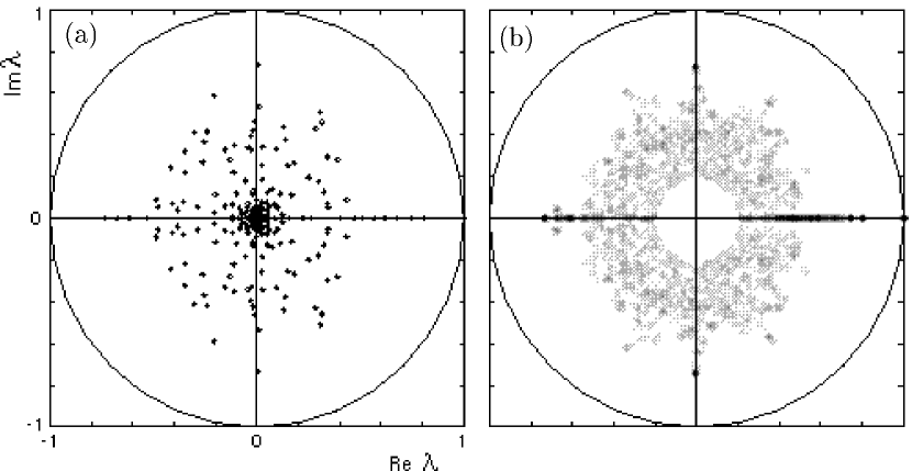
Figure 1: (a) Eigenvalues of the truncated Frobenius-Perron matrix ($l_{\rm max}=32$). (b) Eigenvalue density computed from Frobenius-Perron matrices with $l_{\rm max}=20,21,\dots 70$. The centered disc is not shown, because of the increasing density at the origin (see (a)).

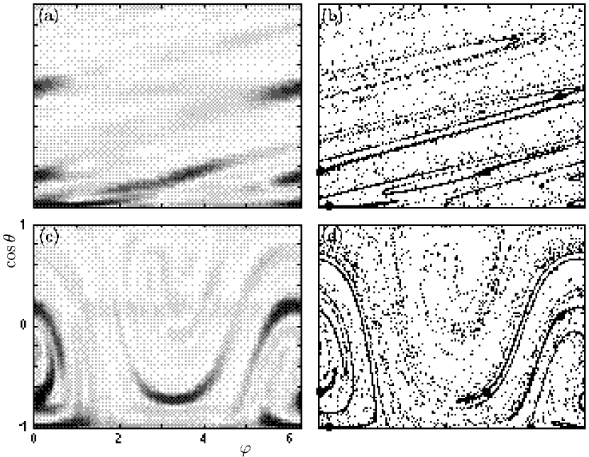
Figure 2: (a) Grey-shade coded phase-space plot of the modulus of the approximate resonance eigenfunction ($l_{\rm max}=32$) from $\lambda\approx-{\rm i}0.75$ (No 4 in Tab. 1). (b) Unstable manifold of a weakly unstable period-4 orbit (spots) supporting the resonance eigenfunction. (c) Approximate resonance eigenfunction of backward time evolution from same resonance as in (a). (d) Stable manifold of the same orbit as in (b).

Fig. 1 (a) shows the eigenvalues of the truncated Frobenius-Perron matrix in the complex plane. Here the dimension is $M=(l_{\rm max}+1)^{2}$, where $l_{\rm max}$ is the maximal total angular momentum of the spherical harmonics in which the density functions are expanded. In (b) we see a grey-scale shaded plot of the eigenvalue density calculated from truncated matrices ($l_{\rm max}=20,21,\dots,70$). Dark spots corresponding to large amplitudes of the density indicate resonance positions, since resolution independent eigenvalues highly increase the density through accumulation. A comparison of both shows that some eigenvalues in (a) reflect resonance positions (see also Tab. 1). In Fig. 2 (a) the modulus of the approximate eigenfunction is plotted in phase space, where the dark regions belong to large moduli of the complex-valued function. The comparison with the unstable manifolds (b) of a weakly unstable period-4 orbit shows that the approximate eigenfunction scars along these manifolds. In (c) and (d) we see the scarring of the eigenfunction of backward time propagation (same resonance as in (a)) along the stable manifolds.

5 Coherent-State Representation

To represent quantum operators in a way close the corresponding classical observables it is convenient to start from coherent states. For the $SU(2)$ group coherent states can be generated by a rotation of the state $|j,m=j\rangle$ as $|\theta,\varphi\rangle=R(\theta,\varphi)|jj\rangle$. In the $|jm\rangle$ basis these coherent states are given by

$$|\theta,\varphi\rangle=\left(1+\left(\tan\frac{{}_{\theta}}{{}^{2}}\right)^{2}\right)^{-j}\sum_{m=-j}^{j}\sqrt{2j\choose j-m}\left(\tan\frac{{}_{\theta}}{{}^{2}}\,{\rm e}^{{\rm i}\varphi}\right)^{j-m}|jm\rangle\,.$$ (12)

Since the set of the coherent states is overcomplete, there are several ways describing quantum operators with coherent states [25, 26, 27]. On the one hand, one can use the so-called $P$ function, defined as the weight of coherent-state projectors in the continuous mixture

$$A=\frac{N}{4\pi}\int{\rm d}\Omega\,P_{A}(\theta,\varphi)\,|\theta,\varphi\rangle\langle\theta,\varphi|\,.$$ (13)

The integral is over the unit sphere, where ${\rm d}\Omega={\rm d}\varphi\,{\rm d}\theta\,\sin\theta$. On the other hand, we have the so-called $Q$ function, the coherent state expectation value of an operator, $Q_{A}(\theta,\varphi)=\langle\theta,\varphi|A|\theta,\varphi\rangle$. It is important that $Q$ is a smooth function on phase space, while $P$ can strongly oscillate, particularly in the shortest wave lengths. However, in contrast to the coherent states of Weyl groups, $P$ functions always exist. Both functions can be expanded in terms of spherical harmonics [28],

$$Q_{A}(\theta,\varphi) = \sum\limits_{l=0}^{2j}\sum\limits_{m=-l}^{l}q_{lm}(A)Y_{l}^{m}(\theta,\varphi)$$

$$P_{A}(\theta,\varphi) = \sum\limits_{l=0}^{2j}\sum\limits_{m=-l}^{l}p_{lm}(A)Y_{l}^{m}(\theta,\varphi)\,,$$ (14)

where the summations break off at the total angular momentum $l=2j$. The Hilbert space of phase-space functions must not be confused with the Hilbert space of quantum wave functions; we therefore use round brackets for the scalar product already introduced in (7), $\mbox{\bf(}\,f\mbox{$|\!\!|$}\,g\mbox{\bf)}=\int{\rm d}\Omega\,f^{\ast}(\theta,\varphi)g(\theta,\varphi)$. Although the $P$ functions tend to oscillate more strongly than the $Q$ functions, the expansion coefficients of the $P$ and $Q$ functions corresponding to the same operator converge to one another in the classical limit, $p_{lm}(A)\mbox{$\,{}_{{}_{N\rightarrow\infty}}\!\!\!\!\!\!\!\!\!\!\!\!\longrightarrow\,$}q_{lm}(A)$ for fixed $l,m$. It is easy to see that the trace of an operator product can be written as the scalar product of $P$ and $Q$ as ${\rm tr}A^{\dagger}B=\frac{N}{4\pi}\mbox{\bf(}P_{A}\mbox{$|\!\!|$}Q_{B}\mbox{\bf)}$. In particular, if the set $\{|\phi_{k}\rangle\}$ of wave functions form an orthogonal basis of the quantum Hilbert space, then the $P$ and $Q$ functions of ket-bras $P_{ik}\equiv P_{|\phi_{i}\rangle\!\langle\phi_{k}|}$ and $Q_{ik}\equiv Q_{|\phi_{i}\rangle\!\langle\phi_{k}|}$ generate biorthonormal sets in the Hilbert space of phase-space functions

$$\frac{N}{4\pi}\mbox{\bf(}P_{ik}\mbox{$|\!\!|$}Q_{i^{\prime}k^{\prime}}\mbox{\bf)}={\rm tr}\left(|\phi_{k}\rangle\!\langle\phi_{i}||\phi_{i^{\prime}}\rangle\!\langle\phi_{k^{\prime}}|\right)=\delta_{kk^{\prime}}\delta_{ii^{\prime}}\,.$$ (15)

The $Q$ function of a density operator $Q_{\rho}$ is also called Husimi function. If the density operator is a projector of form $|\psi\rangle\langle\psi|$ the corresponding Husimi function is a phase-space representation of a quantum wave function. We call the $Q_{ik}\equiv Q_{|\phi_{i}\rangle\!\langle\phi_{k}|}$ Husimi eigenfunction if the $|\phi_{i}\rangle$ denote Floquet eigenstates. The latter notation becomes obvious in the next section. We further distinguish between diagonal Husimi eigenfunctions $Q_{kk}$ and skew ones $Q_{ik}$ with $i\neq k$.

6 Husimi Propagator

The Husimi propagator ${\cal F}$ is defined through the time evolution of a quantum density operator $\rho$ as

$$Q_{\rho(n)}(\theta,\varphi)=\langle\theta,\varphi|F^{n}\rho(0)(F^{\dagger})^{n}|\theta,\varphi\rangle={\cal F}^{n}Q_{\rho(0)}(\theta,\varphi)\,.$$ (16)

Using the Floquet eigenstates, $F|\phi_{i}\rangle={\rm e}^{-{\rm i}\phi_{i}}|\phi_{i}\rangle$, the Husimi eigenfunctions are easily calculated as $Q_{ik}\equiv\langle\theta,\varphi|\phi_{i}\rangle\langle\phi_{k}|\theta,\varphi\rangle$. The Husimi propagator thus has $N^{2}$ unimodular eigenvalues whose phases are differences of the Floquet eigenphases. There is an $N$-fold degeneracy of the eigenvalue $1$ corresponding to the diagonal Husimi eigenfunctions $Q_{kk}$ which are real and normalized as $\int{\rm d}\Omega\,Q_{kk}=4\pi/N$. All other (skew) Husimi eigenfunctions with $i\neq k$ are complex and their phase space-integral vanishes. In basis of spherical harmonics the Husimi propagator becomes an $N^{2}\times N^{2}$ matrix (Husimi matrix). The diagonal representation of the Husimi propagator is simply given as

$${\cal F}^{n}=\frac{2j+1}{4\pi}\sum_{i=0}^{2j}\sum_{k=0}^{2j}\mbox{$|\!\!|$}Q_{ik}\mbox{\bf)}{\rm e}^{-{\rm i}n(\phi_{i}-\phi_{k})}\mbox{\bf(}P_{ik}\mbox{$|\!\!|$}\,.$$ (17)

The Husimi spectral density is identified as the density-density correlation function with respect to the Floquet eigenphases,

$$C(\omega)=\int_{0}^{2\pi}{\rm d}\phi\rho(\omega+\phi)\rho(\phi)=\sum_{ik}\delta(\omega-(\phi_{i}-\phi_{k}))\,,$$ (18)

where $\rho(\phi)=\sum_{k}\delta(\phi-\phi_{k})$. Some authors prefer the normalized density $\tilde{\rho}(\omega)=N^{-1}\sum_{k}\delta(\phi-\phi_{k})$.

7 $L^{2}$ Norms of Husimi Eigenfunctions

The squared $L^{2}$ norm of a diagonal Husimi eigenfunction,

$$||Q_{kk}||^{2}=\int{\rm d}\Omega\,|\langle\theta,\varphi|\phi_{k}\rangle|^{4}\,,$$ (19)

is the inverse participation ratio (IPR) with respect to coherent states (phase-space distribution). It becomes large if the Husimi function is strongly localized in phase space, say scarred on periodic orbits. On the other hand, the squared $L^{2}$ norm of a skew Husimi eigenfunction can be understood as the overlap of two diagonal Husimi functions on phase space,

$$\int{\rm d}\Omega\,|Q_{ik}|^{2}=\int{\rm d}\Omega\,|\langle\theta,\varphi|\phi_{i}\rangle|^{2}|\langle\theta,\varphi|\phi_{k}\rangle|^{2}\,.$$ (20)

From the Schwarz inequality,

$$||Q_{ik}||^{2}\leq||Q_{ii}||\,||Q_{kk}||\,,$$ (21)

it becomes obvious that for large values of $||Q_{ik}||^{2}$ both diagonal Husimi eigenfunctions must be localized in the same phase-space regions.

We illustrate two examples. A constant function on the sphere is of course a uniformly distributed function. But note that it is not a Husimi eigenfunction, since the corresponding density operator is of form $\rho=\frac{1}{N}{\bf 1}$. Using the normalization $\frac{N}{4\pi}\int{\rm d}\Omega\,Q_{\rho}=1$ the Husimi function becomes $\frac{1}{N}$. For the squared $L^{2}$ norm we find

$$||Q_{\rho}||^{2}=\frac{4\pi}{N^{2}}$$ (22)

for uniform function. In comparison, the random-matrix averaged squared $L^{2}$ norms of diagonal Husimi eigenfunctions is larger by a factor 2 (see Sec. 8) which can be explained by quantum fluctuations. A most strongly localized Husimi function, in contrast, corresponds to a density oparator which is a coherent-state projector. Due to the invariance under rotations the $L^{2}$ norm is the same for all coherent-state Husimi functions. Using the coherent-state projector $|jj\rangle\langle jj|$ and (LABEL:exaktl2) one easily finds for the squared $L^{2}$ norm

$$||Q_{|jj\rangle\!\langle jj|}||^{2}=\frac{2\pi}{N}$$ (23)

for strongly localized Husimi function. It becomes obvious that squared $L^{2}$ norms of most strongly localized and uniformly distributed Husimi functions differ by a factor of order $N$.

We here show the calculation of the $L^{2}$ norm from vector coefficients in the $|jm\rangle$ basis ($c^{k}_{m}=\langle jm|\phi_{k}\rangle$). Introducing the decomposition of unity in terms of the angular momentum states, ${\bf 1}=\sum_{m=-j}^{j}|jm\rangle\langle jm|$, the $L^{2}$ norm of a skew Husimi eigenfunction becomes a four-fold sum,

$$\int{\rm d}\Omega\,|\langle\theta,\varphi|\phi_{i}\rangle\langle\phi_{k}|\theta,\varphi\rangle|^{2} = \sum_{m_{1}\dots m_{4}}c^{i}_{m_{1}}(c^{i}_{m_{2}})^{\ast}c^{k}_{m_{3}}(c^{k}_{m_{4}})^{\ast}$$ (24)

$$\times\int{\rm d}\Omega\,\langle\theta,\varphi|jm_{1}\rangle\langle jm_{2}|\theta,\varphi\rangle\langle\theta,\varphi|jm_{3}\rangle\langle jm_{4}|\theta,\varphi\rangle\,.$$

From the definition (12) of the coherent states we find, using the relations $\tan\frac{\theta}{2}=\frac{1-\cos\theta}{\sin\theta}=\frac{\sin\theta}{1+\cos\theta}$ for $0\leq\theta\leq\pi$,

$$\langle jm|\theta,\varphi\rangle=2^{-j}\sqrt{2j\choose j-m}(1-\cos\theta)^{\frac{j-m}{2}}(1+\cos\theta)^{\frac{j+m}{2}}{\rm e}^{{\rm i}(j-m)\varphi}\,.$$ (25)

After a few further steps the phase-space integral $\int{\rm d}\Omega\,=\int_{0}^{\pi}{\rm d}\theta\,\sin\theta\int_{0}^{2\pi}{\rm d}\varphi$ leads to a Kronecker $\delta$ and to a beta function [29] for the $\varphi$- and $\theta$-dependent part, respectively. We thus obtain for the coefficients of the summation (24)

$$\int{\rm d}\Omega\,\langle\theta,\varphi|jm_{1}\rangle\langle jm_{2}|\theta,\varphi\rangle\langle\theta,\varphi|jm_{3}\rangle\langle jm_{4}|\theta,\varphi\rangle$$

$$=4\pi\frac{\Gamma(\frac{4j-\sum m_{i}}{2}+1)\Gamma(\frac{4j+\sum m_{i}}{2}+1)}{\Gamma(4j+2)}$$

$$\times\delta(m_{1}\!-\!m_{2}\!+\!m_{3}\!-\!m_{4})\sqrt{{2j\choose j-m_{1}}{2j\choose j-m_{2}}{2j\choose j-m_{3}}{2j\choose j-m_{4}}}$$ (26)

We make use of the argument of the Kronecker $\delta$ and get for the $L^{2}$ norm

$$\int{\rm d}\Omega\,|\langle\theta,\varphi|\phi_{i}\rangle\langle\phi_{k}|\theta,\varphi\rangle|^{2} = 4\pi\sum_{m_{1}\dots m_{4}}\frac{(2j-m_{1}-m_{3})!(2j+m_{1}+m_{3})!}{(4j+1)!}$$

$$\times \sqrt{{2j\choose j-m_{1}}{2j\choose j-m_{2}}{2j\choose j-m_{3}}{2j\choose j-m_{4}}}$$

$$\times \delta(m_{1}\!-\!m_{2}\!+\!m_{3}\!-\!m_{4})c^{i}_{m_{1}}(c^{i}_{m_{2}})^{\ast}c^{k}_{m_{3}}(c^{k}_{m_{4}})^{\ast}\,.$$

The latter formular will be used for the calculation of Husimi $L^{2}$ norms of random vectors in the next section.

8 Random-Matrix Average of $L^{2}$ Norms

In order to compare the results of the kicked top with those of random-matrix theory we now consider diagonal Husimi eigenfunctions and replace the coefficients by real or complex random numbers due to the orthogonal (COE) or unitary ensemble (CUE), respectively [30]. It is easy to see from (19,20) that the $L^{2}$ norm of a Husimi function is invariant under rotations. As it has been shown in Sec. 2 the eigenvectors of the kicked top must be compared to real random vectors. The only correlation between the coefficients is the normalization of the vector, $\sum_{m}|c_{m}|^{2}=1$ (we drop the upper index in the following). Therefore we neglegt all terms containing random phases and keep the contributing terms with $m_{1}=m_{2}\wedge m_{3}=m_{4}$ or $m_{1}=m_{4}\wedge m_{2}=m_{3}$. By the choice of real coefficients one has the further possibility $m_{1}=m_{3}\wedge m_{2}=m_{4}$. We may abbreviate the coefficients of the summation (26) as $f(m_{1},\dots,m_{4})$ for a moment to find out the contributing terms,

$$\left\langle||Q_{kk}||^{2}\right\rangle = \sum_{m_{1}\dots m_{4}}f(m_{1},\dots,m_{4})\,\delta(m_{1}\!-\!m_{2}\!+\!m_{3}\!-\!m_{4})\left\langle c_{m_{1}}c_{m_{2}}^{\ast}c_{m_{3}}c_{m_{4}}^{\ast}\right\rangle$$

$$= \sum_{m_{1}\dots m_{4}}f(m_{1},\dots,m_{4})\,\delta(m_{1}\!-\!m_{2}\!+\!m_{3}\!-\!m_{4})$$

$$\times \!\!\bigg{(}\Big{[}\delta_{m_{1}m_{2}}\delta_{m_{3}m_{4}}(1-\delta_{m_{1}m_{3}})+\delta_{m_{1}m_{4}}\delta_{m_{2}m_{3}}(1-\delta_{m_{1}m_{3}})$$

$$+ \!\!\{\delta_{m_{1}m_{3}}\delta_{m_{2}m_{4}}(1-\delta_{m_{1}m_{2}})\}\Big{]}\left\langle|c_{m}|^{2}|c_{n}|^{2}\right\rangle+\delta_{m_{i}m_{k}}^{3}\left\langle|c_{m}|^{4}\right\rangle\!\bigg{)}\,.$$

The diagonal part $\delta_{m_{i}m_{k}}^{3}=\delta_{m_{1}m_{2}}\delta_{m_{2}m_{3}}\delta_{m_{3}m_{4}}$ is separated, since there appears the average of $|c_{m}|^{4}$. Due to the symmetry of $f(m_{1},\dots,m_{4})$ the first two terms in the bracket give the same contribution; to that end, one executes the summations over $m_{2}$ and $m_{4}$. The contribution coming from real coefficients $\{\dots\}$ vanishes; here one summates over $m_{3}$ and $m_{4}$. Finally, one finds for the averaged $L^{2}$ norm

$$\left\langle||Q_{kk}||^{2}\right\rangle = \frac{4\pi}{4j+1}\bigg{[}2\sum_{m,n=-j\atop m\neq n}^{j}{4j\choose 2j-m-n}^{-1}{2j\choose j-m}{2j\choose j-n}\left\langle|c_{m}|^{2}|c_{n}|^{2}\right\rangle$$ (29)

$$+ \sum_{m=-j}^{j}{4j\choose 2j-2m}^{-1}{2j\choose j-m}^{2}\left\langle|c_{m}|^{4}\right\rangle\bigg{]}\,.$$

Next we need the averages of products,

$$\left\langle|c_{m}|^{2}|c_{n}|^{2}\right\rangle = \left\{\begin{array}[]{cc}\frac{1}{N(N+1)}&,\,{\rm CUE}\\ \frac{1}{N(N+2)}&,\,{\rm COE}\end{array}\right.\,,$$ (32)

$$\left\langle|c_{m}|^{4}\right\rangle = \left\{\begin{array}[]{cc}\frac{2}{N(N+1)}&,\,{\rm CUE}\\ \frac{3}{N(N+2)}&,\,{\rm COE}\end{array}\right.\,.$$ (35)

The averages are easily calculated from the probability distribution given in [30]. It should be remarked here that semiclassical corrections are of next to leading order of $N^{-1}$. Therefore we do not neglect this order in our RMT results.

Let us consider first the CUE. Since $\left\langle|c_{m}|^{4}\right\rangle=2\left\langle|c_{m}|^{2}|c_{n}|^{2}\right\rangle$, we can complete the summations over the diagonal $(m=n)$ and off-diagonal $(m\neq n)$ part. Thus we have for the CUE

$$\left\langle||Q_{kk}||^{2}\right\rangle=\frac{8\pi}{N(N+1)}\frac{1}{4j+1}\sum_{m,n=-j}^{j}{4j\choose 2j-m-n}^{-1}{2j\choose j-m}{2j\choose j-n}\,.$$ (36)

It might not be easy to see that this results to $\left\langle||Q_{kk}||^{2}\right\rangle=\frac{8\pi}{N(N+1)}$. To that end we present an alternative way to calculate the averaged $L^{2}$ norm which is unfortunately not applicable for the COE [6]. An arbitrary complex random vector can be written as $|\psi\rangle=U|jj\rangle$, where $U$ is a unitary random matrix. A coherent state is generated through a rotation operator as $|\theta,\varphi\rangle=R(\theta,\varphi)|jj\rangle$. We thus have $\langle\theta,\varphi|\psi\rangle=\langle jj|R^{\dagger}U|jj\rangle$. The product $R^{\dagger}U=\tilde{U}$ defines a new unitary random matrix, where the Haar measure keeps unchanged ${\rm d}\mu(\tilde{U})={\rm d}\mu(U)$. Therefore the averaged $L^{2}$ norm becomes

$$\left\langle||Q_{kk}||^{2}\right\rangle = \int{\rm d}\mu(U)\int{\rm d}\Omega\,|\langle jj|R^{\dagger}U|jj\rangle|^{4}$$ (37)

$$= \int{\rm d}\Omega\int{\rm d}\mu(\tilde{U})\,|\langle jj|\tilde{U}|jj\rangle|^{4}$$

$$= 4\pi\left\langle|c_{m}|^{4}\right\rangle\,.$$

Note that for the COE, in contrast, one deals with real vectors which generally become complex after rotating.

For the COE we again complete the diagonal and off-diagonal summations in (29), whereby a further contribution remains, because of the factor $3$ of the fourth moment (35),

$$\frac{4\pi}{4j+1}\sum_{m=-j}^{j}{4j\choose 2j-2m}^{-1}{2j\choose j-m}^{2}\frac{1}{N(N+2)}=\frac{(4^{j}(2j)!)^{2}}{(4j+1)(4j)!}\,\frac{4\pi}{N(N+2)}\;\;\;$$ (38)

The latter equation can be calculated as follows [32]. We rewrite

$$\sum_{m=-j}^{j}{4j\choose 2j-2m}^{-1}{2j\choose j-m}^{2}=\frac{(2j)!^{2}}{(4j)!}\sum_{k=0}^{2j}{2k\choose k}{4j-2k\choose 2j-k}$$ (39)

with $k=m+j$. We now show that

$$\sum_{k=0}^{n}{2k\choose k}{2n-2k\choose n-k}=4^{n}\,.$$ (40)

The generating function of ${2k\choose k}$ is

$$\frac{1}{\sqrt{1-4x}}=\sum_{k=0}^{\infty}{2k\choose k}x^{k}$$ (41)

which is easily seen from Taylor expansion,

$$\frac{1}{k!}\frac{{\rm d}^{k}}{{\rm d}x^{k}}(1-4x)^{-\frac{1}{2}}\bigg{|}_{x=0}=\frac{1}{k!}\frac{1}{2}\left(1+\frac{1}{2}\right)\dots\left(k-\frac{1}{2}\right)4^{k}=\frac{(2k)!}{k!^{2}}\,.$$ (42)

Squaring the generating function gives

$$\frac{1}{1-4x}=\sum_{k=0}^{\infty}\sum_{l=0}^{\infty}{2k\choose k}{2l\choose l}x^{k+l}=\sum_{n=0}^{\infty}x^{n}\sum_{k=0}^{n}{2k\choose k}{2n-2k\choose n-k}\,,$$ (43)

where $n=k+l$. Comparing the latter equation with the geometric series

$$\frac{1}{1-4x}=\sum_{n=0}^{\infty}x^{n}4^{n}$$ (44)

finishes the proof.

The aforementioned contribution (38) becomes more familiar by the approximation

$$\frac{(4^{j}(2j)!)^{2}}{(4j+1)(4j)!}=\frac{\sqrt{\pi}}{2}\frac{\Gamma(2j+1)}{\Gamma(2j+3/2)}\approx\frac{1}{2}\sqrt{\frac{\pi}{2j+1}}\,.$$ (45)

The averaged $L^{2}$ norms finally become

$$\left\langle||Q_{kk}||^{2}\right\rangle\simeq\frac{4\pi}{N^{2}}\left\{\begin{array}[]{cc}\frac{2N}{N+1}&,\,{\rm CUE}\\ \frac{N}{N+2}\left(2+\frac{1}{2}\sqrt{\frac{\pi}{N}}\right)&,\,{\rm COE}\end{array}\right.\,,$$ (46)

As an interesting point to remark here the COE eigenstates are somewhat more localized than the CUE eigenstates, since their averaged $L^{2}$ norm contains a further contribution of order $N^{-\frac{5}{2}}$. But in contrast to the fourth moment (35) - it might be understood as the averaged IPR with respect to the $|jm\rangle$ basis - the difference vanishes in the classical limit $N\rightarrow\infty$. However, for both ensembles the averaged squared $L^{2}$ norms are roughly twice larger than for a constant distribution on the sphere.

For the skew Husimi eigenfunctions the averaged $L^{2}$ norms can be calculated from the relation

$$4\pi=\int{\rm d}\Omega\,|\langle\theta,\varphi|\theta,\varphi\rangle|^{2}=\int{\rm d}\Omega\,\left(\sum_{k}|\langle\theta,\varphi|\phi_{k}\rangle|^{2}\right)^{2}=\sum_{k}||Q_{kk}||^{2}+\sum_{i\neq k}||Q_{ik}||^{2}\,,$$ (47)

which leads to

$$\left\langle||Q_{ik}||^{2}\right\rangle=\frac{4\pi-N\left\langle||Q_{kk}||^{2}\right\rangle}{N(N-1)}\,.$$ (48)

Introducing the averages of the diagonal ones we find for CUE

$$\left\langle||Q_{ik}||^{2}\right\rangle=\frac{4\pi}{N^{2}}\frac{N}{N+1}\,.$$ (49)

For the COE one obtaines the same result up to an order of $N^{-\frac{7}{2}}$,

$$\left\langle||Q_{ik}||^{2}\right\rangle\simeq\frac{4\pi}{N^{2}}\frac{N^{2}}{(N-1)(N+2)}\left(1-\frac{1}{2N}\sqrt{\frac{\pi}{N}}\right)=\frac{4\pi}{N^{2}}\frac{N}{N+1}+{\cal O}(N^{-\frac{7}{2}})\,.$$ (50)

9 Comparison of Quantum and Classical Eigenfunctions

It has been shown in [31] that quantum quasiprobability propagation looks classical if phase-space resolution is blurred such that Planck cells are far from being resolved. As a result, if we truncate the Husimi matrix to coarse phase-space resolution, then it becomes almost equal to the truncated Frobenius-Perron operator, $T{\cal F}T\mbox{$\,{}_{{}_{N\rightarrow\infty}}\!\!\!\!\!\!\!\!\!\!\!\!\longrightarrow\,$}T{\cal P}T$, where

$$T=\sum_{l=0}^{l_{\rm max}}\sum_{m=-l}^{l}\mbox{$|\!\!|$}Y_{l}^{m}\mbox{\bf)}\mbox{\bf(}Y_{l}^{m}\mbox{$|\!\!|$}$$ (51)

denotes the truncation projector restricting the “classical” Hilbert space dimension to $M=(l_{\rm max}+1)^{2}$. In the following we choose $M\ll N^{2}$, and thus have $T{\cal F}T\approx T{\cal P}T$. Again we consider the classical propagator. Let $\mbox{$|\!\!|$}w\mbox{\bf)}=T\mbox{$|\!\!|$}w\mbox{\bf)}$ be an approximate resonance eigenfunction with stabilized eigenvalue $\lambda$ of $T{\cal P}T$. Since the stabilized eigenvalues reflect spectral properties of the non-truncated Frobenius-Perron operator, $\lambda^{n}$ must be a stabilized eigenvalue of $T{\cal P}^{n}T$, at least if $M$ is chosen large enough. This property does not hold for non-stabilized eigenvalues, since $T{\cal P}^{n}T\neq(T{\cal P}T)^{n}$. Choosing the approximate resonance eigenfunction $L^{2}$ normalized, the return probability becomes $\mbox{\bf(}w\mbox{$|\!\!|$}{\cal P}\mbox{$|\!\!|$}w\mbox{\bf)}=\lambda^{n}$ for small $n$ (see Fig. 3). Note that the latter property makes sense only if we consider approximate resonance eigenfunctions, because the singular resonance eigenfunctions are not square integrable. Fig. 3 shows the return probability of the approximate eigenfunction from stabilized eigenvalue $\lambda_{\nu}\approx-{\rm i}0.75$ (No 4 in Tab. 1). As well the moduli as the phases coincide with $\lambda_{\nu}^{n}$ for about 20 iterations. Beyond this time quantum fluctuations become visible.

Since $T{\cal F}T\approx T{\cal P}T$, we expect $T{\cal F}^{n}T\approx T{\cal P}^{n}T$ for small $n$. Now we can replace the Husimi propagator by its diagonal representation (17),

$$\lambda^{n}\approx\mbox{\bf(}w\mbox{$|\!\!|$}{\cal F}^{n}\mbox{$|\!\!|$}w\mbox{\bf)}=\frac{N}{4\pi}\sum_{ik}\mbox{\bf(}w\mbox{$|\!\!|$}Q_{ik}\mbox{\bf)}{\rm e}^{-{\rm i}n(\phi_{i}-\phi_{k})}\mbox{\bf(}P_{ik}\mbox{$|\!\!|$}w\mbox{\bf)}\,.$$ (52)

The return probability becomes a double sum of overlaps of quantum and classical eigenfunctions. For large $N$ the Husimi eigenphases are quite dense in the interval $[0,2\pi)$. Outside an interval around the Husimi eigenphase $\omega=0$ wherein level repulsion of Floquet eigenphases become perceptible the spectral density of differences $\phi_{i}-\phi_{k}$ is almost constant, $N^{2}/2\pi$. It is convenient to replace the sum by a continuous integral over the Husimi eigenphases, where the overlaps can be replaced by a continuous function as a smoothed distribution of overlaps,

$$\lambda^{n}\approx\frac{N}{4\pi}\int\limits_{0}^{2\pi}{\rm d}\omega\,\overline{\mbox{\bf(}w\mbox{$|\!\!|$}Q_{ik}\mbox{\bf)}\mbox{\bf(}P_{ik}\mbox{$|\!\!|$}w\mbox{\bf)}}^{\Delta\omega}(\omega){\rm e}^{-{\rm i}n\omega}\,.$$ (53)

In the classical limit we let first $N\longrightarrow\infty$ and then $M\longrightarrow\infty$. In this limit the foregoing result becomes valid for all $n$. The smoothed overlaps are given by the inverse Fourier transform of $\lambda^{n}$ as

$$\overline{\mbox{\bf(}w\mbox{$|\!\!|$}Q_{ik}\mbox{\bf)}\mbox{\bf(}P_{ik}\mbox{$|\!\!|$}w\mbox{\bf)}}^{\Delta\omega}(\omega)\mbox{$\,{}_{{}_{N\rightarrow\infty}}\!\!\!\!\!\!\!\!\!\!\!\!\longrightarrow\,$}\frac{2}{N}\frac{1-|\lambda|^{2}}{1+|\lambda|^{2}-2|\lambda|\cos(\omega-\arg\lambda)}\,,$$ (54)

which is a periodic “Lorentzian” displaced by the phase of $\lambda$ and of width $-\ln|\lambda|$ [33] (see Fig. 4).

The smoothing is done by a convolution with a sinc function which naturally results from a truncated Fourier transform. Here the time restriction is ${\cal N}\leq n\leq{\cal N}$, where ${\cal N}\approx 20$ corresponding to the validity of the return probability of the approximate eigenfunction (Fig. 4). For simplification the integral is restricted on the interval between the first zeros of the sinc function,

$$\overline{f}^{\Delta\omega}(\omega)\propto\int\limits_{\omega-\frac{\pi}{\cal N}}^{\omega+\frac{\pi}{\cal N}}{\rm d}\omega^{\prime}\frac{\sin({\cal N}\omega^{\prime})}{\omega^{\prime}}f(\omega-\omega^{\prime})\,.$$ (55)

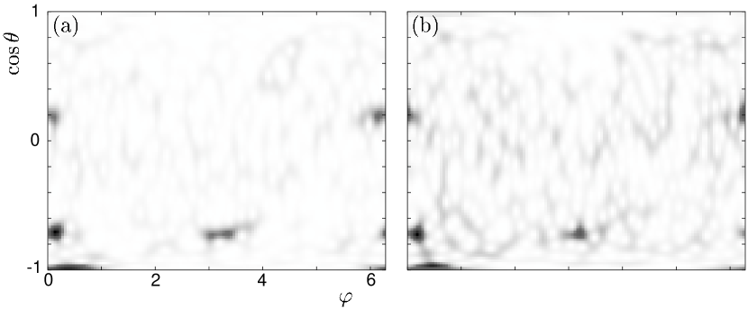
Figure 5: Grey-shade coded phase-space plots of the diagonal Husimi eigenfunctions (a) No 30 and (b) No 11 of Tab. 3. The Husimi function in (a) is strongly scarred in phase-space regions, where the approximate resonance eigenfunctions are scarred (Fig. 2). The Husimi function in (b) is also scarred in the same phase-space regions, but shows more structures all over the phase space than the function in (a).

A simple argument connects quantum scars with Ruelle-Pollicott resonances. Classical resonance eigenfunctions are scarred along unstable manifolds (or stable manifolds for backward time propagation). Quantum eigenfunctions which strongly overlap with resonance eigenfunctions have to be scarred as well. This is an important result, because it explains scarring of quantum eigenfunctions not only on periodic orbits, but also along stable and unstable manifolds. This has been observed for the kicked top [34]. For instance, we consider the skew Husimi eigenfunction which shows the largest overlap with the classical approximate eigenfunction considered before. The corresponding diagonal Husimi eigenfunctions (No 11 and No 30 in Tab. 3) plotted in Fig. 5 are scarred in the same phase-space regions, where the the approximate resonance eigenfunctions are scarred (Fig. 2), while the difference of their Floquet eigenphases ($\phi_{30}-\phi_{11}=-1.586$) is close to the phase of the resonance ($\arg\lambda_{4}=-\frac{\pi}{2}$).

10 Resonance Corrections of Averaged Phase-Space Overlaps

In the foregoing section a qualitative explenation of the connection between resonances and quantum eigenfunctions was given, but now we are interested in more quantitative results. To that end, we consider transition rates of coherent states in the classical limit

$$\frac{N}{4\pi}|\langle\theta,\varphi|F^{n}|\theta^{\prime},\varphi^{\prime}\rangle|^{2}\mbox{$\,{}_{{}_{N\rightarrow\infty}}\!\!\!\!\!\!\!\!\!\!\!\!\longrightarrow\,$}\delta\left((q,p)-{\cal M}^{n}(q^{\prime},p^{\prime})\right)\,.$$ (56)

The latter relation becomes obvious if one suggests that coherent states are wave functions most strongly localized on phase-space points. We now consider the return probability and integrate over the phase space,

$$\frac{N}{4\pi}\int{\rm d}\Omega\,|\langle\theta,\varphi|F^{n}|\theta,\varphi\rangle|^{2}\mbox{$\,{}_{{}_{N\rightarrow\infty}}\!\!\!\!\!\!\!\!\!\!\!\!\longrightarrow\,$}\int{\rm d}\Omega\,\delta\left((q,p)-{\cal M}^{n}(q,p)\right)\,,$$ (57)

where the rhs is the trace of the Frobenius-Perron operator [37]. We remark here that the integral on the rhs leads to a sum of contributions from periodic orbits, which is an important connection between scars on periodic orbits and the results of our paper. On the one hand, periodic orbits, in particular the weakly unstable ones, contribute to the trace of the Frobenius-Perron operator, i.e. influence the resonances. On the other hand, scars typically appear around weakly unstable periodic orbits. On the lhs of (57) we introduce the diagonal representation of the Floquet operator and get

$$\frac{N}{4\pi}\int{\rm d}\Omega\,|\langle\theta,\varphi|F^{n}|\theta,\varphi\rangle|^{2} = \frac{N}{4\pi}\int{\rm d}\Omega\,\left|\sum_{k}|\langle\theta,\varphi|\phi_{k}\rangle|^{2}{\rm e}^{-{\rm i}n\phi_{k}}\right|^{2}$$ (58)

$$= \frac{N}{4\pi}\sum\limits_{ik}||Q_{ik}||^{2}\,{\rm e}^{-{\rm i}n(\phi_{i}-\phi_{k})}\,.$$

Fourier transformation of the latter expression leads to a sum of $\delta$ functions weighted by $L^{2}$ norms,

$$\sum\limits_{n=-\infty}^{\infty}\frac{{\rm e}^{{\rm i}n\omega}}{2\pi}\sum\limits_{ik}||Q_{ik}||^{2}\,{\rm e}^{-{\rm i}n(\phi_{i}-\phi_{k})}=\sum\limits_{ik}||Q_{ik}||^{2}\,\delta(\omega-(\phi_{i}-\phi_{k}))\,.$$ (59)

Due to the arguments of the foregoing section we expect that for finite $N$ the relation (56) is valid for finite times $|n|\leq{\cal N}$. Validity of semiclassical methods is guarantied for times up to the Ehrenfest time, where the number of fixpoints coincides with the number of Planck cells. Thus we identify ${\cal N}$ as Ehrenfest time. The truncated Fourier transform leads to a sum of smoothed $\delta$ functions (55). Using (57) we get

$$\overline{||Q_{ik}||^{2}}^{\Delta\omega}(\omega)=\frac{4\pi}{N}\sum_{n=-{\cal N}}^{\cal N}{\rm tr}{\cal P}^{n}\frac{{\rm e}^{{\rm i}n\omega}}{2\pi}\,$$ (60)

which we may call smoothed $L^{2}$ norms. The next step is to drop the stationary eigenvalue $1$ in the traces of the Frobenius-Perron operator. The Fourier transform of this eigenvalue leads to a $\delta$ function in the limit ${\cal N}\rightarrow\infty$ which is not a point of interest here. In the Husimi representation we identify the eigenvalue $1$ as the sum of squared $L^{1}$ norms of Husimi eigenfunctions. This is easily seen from the Husimi matrix in basis of spherical harmonics. In the first row and column is only one non-vanishing matrix element $\mbox{\bf(}Y_{0}^{0}\mbox{$|\!\!|$}{\cal F}\mbox{$|\!\!|$}Y_{0}^{0}\mbox{\bf)}=1$. Note that $Y_{0}^{0}$ is a constant function on the sphere and therefore proportional to the stationary density, i.e. it is the eigenfunction from eigenvalue $1$. Introducing the diagonal representation of the Husimi propagator (17) one identifies $\frac{N}{4\pi}\sum_{k}\mbox{\bf(}Y_{0}^{0}\mbox{$|\!\!|$}Q_{kk}\mbox{\bf)}\mbox{\bf(}P_{kk}\mbox{$|\!\!|$}Y_{0}^{0}\mbox{\bf)}=1$. Note that $\mbox{\bf(}Y_{0}^{0}\mbox{$|\!\!|$}Q_{ik}\mbox{\bf)}=\mbox{\bf(}P_{ik}\mbox{$|\!\!|$}Y_{0}^{0}\mbox{\bf)}=\frac{\sqrt{4\pi}}{N}\delta_{ik}$, where $\mbox{\bf(}Y_{0}^{0}\mbox{$|\!\!|$}Q_{kk}\mbox{\bf)}\propto||Q_{kk}||_{1}$. For $n=0$ the trace of the Frobenius-Perron operator is not defined. The integral on the lhs of (57), however, is defined and gives the leading order contribution $N$. We replace the traces by sums of the Ruelle-Pollicott resonances (10) and make use of the symmetry ${\rm tr}{\cal P}^{-n}={\rm tr}{\cal P}^{n}$,

$$\overline{||Q_{ik}||^{2}}^{\Delta\omega}(\omega)=2\frac{N-1}{N}+\frac{4}{N}\sum_{n=1}^{\cal N}\sum_{\nu}\lambda^{n}_{\nu}\cos n\omega\,.$$ (61)

Note that the eigenvalue $1$ is also dropped in the leading order term.

To get from the smoothed $L^{2}$ norms $\overline{||Q_{ik}||^{2}}^{\Delta\omega}(\omega)$ to a mean value $\left\langle||Q_{ik}||^{2}\right\rangle_{\Delta\omega}(\omega)$ we have to divide it by the smoothed level density of the Husimi spectrum. The density of the Husimi spectrum is identified as the density-density correlation function with respect to the Floquet eigenphases,

$$\rho_{H}(\omega)=\sum_{ik}\delta(\omega-(\phi_{i}-\phi_{k}))\,.$$ (62)

This spectral density can be calculated from the time Fourier transformation of the form factor. The smoothed density is given by a truncated Fourier transformation as

$$\overline{\rho}^{\Delta\omega}(\omega)=\frac{N^{2}}{2\pi}\left(1+\frac{2}{N^{2}}\sum_{n=1}^{\cal N}|{\rm tr}F^{n}|^{2}\cos n\omega\right)\,,$$ (63)

where we have separated the leading order term ($n=0$). It is known that the form factor is small as the time $n$ is small ($\left\langle|{\rm tr}F^{n}|^{2}\right\rangle=n$ or $\approx 2n$ for CUE or COE, respectively). Thus, the summation up to the Ehrenfest time which is much smaller than $N$ becomes negligible and the smoothed spectral density is nearly constant. Before we write down the final result, we consider the truncated Fourier transformation of the resonances. Since the moduli of the resonances are smaller $1$, the summations in (61) converge quickly such that we can replace the Ehrenfest time ${\cal N}$ by $\infty$,

$$\left\langle||Q_{ik}||^{2}\right\rangle(\omega)=\frac{4\pi}{N^{2}}\left(\frac{N-1}{N}+\frac{2}{N}\sum_{\nu}\sum_{n=1}^{\infty}\lambda_{\nu}^{n}\cos n\omega\right)\,.$$ (64)

The constant term coincides with the RMT result (50), where $\frac{N}{N+1}=\frac{N-1}{N}+{\cal O}(N^{-2})$. The resonances lead to an $\frac{1}{N}$ (alias $\hbar$) correction in form of overlapping Lorentz distributions (see (54)). In the classical limit the resonance corrections vanish as $N$ goes to infinity. However, for finite dimension we see non-universal corrections which are related to the chaoticity of the system. If, for instance, the classical dynamics is strongly chaotic such that all correlations vanish after one iteration, the resonances are close to the origin and the averaged $L^{2}$ norms show no deviations from RMT result.

Before we come to numerical results we should discuss some prelimaries. The kicked top is known to have a mixed phase space. Although elliptic islands of stable periodic orbits are much smaller than the Planck cell, bifurcations can be responsible for further localization phenomena which are sometimes called super scars [35]. But in contrast to the resonances, bifurcations strongly influence spectral correlations. That means that peaks resulting from bifurcating orbits are higher for the smoothed $L^{2}$ norms than for the averaged $L^{2}$ norms. Thus, we are able to distinguish between localization phenomena of resonances and bifurcations. The smoothing is again done by a convolution with a sinc function (55). From the contributions of the diagonal Husimi eigenfunctions we have neglegted the squared $L^{1}$ norms which correspond to the stationary eigenvalue.

Fig. 6 shows (a) the smoothed $L^{2}$ norms, (b) the mean $L^{2}$ norms, and (c) the smoothed spectral density. In (a) we see a couple of peaks at the Husimi eigenphases $\omega=0$, $\pi$, $\pm\frac{\pi}{2}$, and $\pm\frac{2\pi}{3}$. In (c) are remarkable peaks at the positions $\omega=\pm\frac{2\pi}{3}$ and after division we see in (b) that these peaks are suppressed, while the other peaks still have the same magnitude. Comparison with the semiclassical prediction is shown in Fig. 7. Due to the fact that stabilized eigenvalues representing the resonances are of largest moduli we expect that the semiclassical prediction is almost independent of the set of eigenvalues as well as all stabilized ones are taken into account. In (a) the semiclassical prediction is computed from (i) eight stabilized eigenvalues, (ii) eigenvalues of modulus larger $0.45$, and (iii) almost all eigenvalues of the truncated Frobenius-Perron matrix. Comparison of (i)–(iii) shows that the semiclassical prediction is mainly influenced from a few classical eigenvalues of large moduli which represent the resonances. In (b) we compare the semiclassical prediction (iii) with the quantum result. In particular for the peaks we find a very good agreement. This result shows that the probability to find strongly overlapping eigenfunctions becomes large if the differences of their eigenphases coincides with the phase of a leading resonance, i.e. resonance of large modulus. In comparison with the background the peaks are small (a few percent). However, we show in the next section that strongly scarred eigenfunctions are mainly responsible for the peaks. The eigenvalues of the Frobenius-Perron matrix (c) are plotted logarithmically ($\ln|\lambda|$ versus $\arg\lambda$). These are easily associated with the peaks in (a). It should be remarked that there is no eigenvalue of large modulus which corresponds to the small peaks at $\omega=\pm\frac{2\pi}{3}$ in Fig. 6 (a).

11 Scarred Eigenstates of the Kicked Top

In this section we consider single eigenfunctions and verify the statement that phase differences of strongly overlapping eigenfunctions coincide with phases of leading resonances. Due to the Schwarz inequality we first check that skew Husimi eigenfunctions with large $L^{2}$ norms are composed by scarred diagonal Husimi eigenfunctions. In Tab. 2 we find 25 $L^{2}$ norms of most strongly localized skew Husimi eigenfunctions, their eigenphases, and the corresponding diagonal Husimi eigenfunctions (the numbers correspond to the enumeration in Tab. 3). Due to the symmetry $Q_{ik}=Q_{ki}^{\ast}$ we have restricted the eigenphases as $0<\omega\leq\pi$. The 32 most strongly localized diagonal Husimi eigenfunctions are presented in Tab. 3. Comparison of both tables proves that all skew Husimi eigenfunctions considered are composed from at least one scarred diagonal eigenfunction. In Fig. 8 (a) $L^{2}$ norms of all diagonal Husimi eigenfunctions are shown, while in (b) we see 530 (of total $1.6\times 10^{5}$) $L^{2}$ norms of most strongly localized skew Husimi eigenfunctions. Due to our foregoing results localized skew Husimi eigenfunctions appear frequently around the resonance phases. Interestingly, there are only two remarkable eigenfunctions (No 11 and 12 in Tab. 2) around the Husimi eigenphases $\omega=\pm\frac{2\pi}{3}$. Moreover, in both cases one of the underlying diagonal Husimi eigenfunctions is No 16 in Tab. 3. Further investigation of this eigenfunction has shown that it is strongly scarred on two bifurcating orbits of periods $1$ and $3$. It seems that we found a super scar corresponding to a period-tripling bifurcation.

12 Conclusion

In conclusion, phase-space localization of quantum (quasi-)eigenenergy functions, say scarring, is not only explained by periodic orbits, but also by Ruelle-Pollicott resonances and their corresponding resonance eigenfunctions. In particular, we found the interesting result that quantum Floquet eigenfunctions are pairwise localized in the same phase-space regions if the difference of their (quasi-)eigenenergies coincides with the phase of a leading resonance, i.e. resonance close to the unit circle. But note that this is a statistical statement which does not make a prediction for individual eigenstates. Moreover, we can not determine if there are either a few strongly scarred or many weakly localized eigenfunctions. However, the semiclassical prediction of the averaged $L^{2}$ norms is in a good agreement with numerical results.

The correspondence between scars around periodic orbits described by Heller and the results of this paper might be understood as follows: resonances can be computed by a so-called cycle expansion, where resonances appear as roots of a polynomial whose coefficients are calculated from contributions of short periodic orbits (pseudo orbits) [36, 37]. On the one hand, scars typically appear around weakly unstable periodic orbits. On the other hand, these weakly unstable orbits mainly induce the cycle expansion.

Although the kicked top has a mixed phase space, localization effects of stable orbits or bifurcations can be neglected if such phase-space structures are not resolved by the Planck cell. Further investigations are needed for the understanding of the so-called super scars which are related to bifurcations.

For fruitful discussions the author thanks Fritz Haake, Karol Życzkowski, Sven Gnutzmann, Joachim Weber, Petr Braun and Pierre Gaspard.

We gratefully acknowledge support by the Sonderforschungsbereich Unordnung und große Fluktuationen of the Deutsche Forschungsgemeinschaft.

$$\begin{array}[]{|r|r|r||r|r|}\hline\cr{\rm No}&{\rm Re}\,\lambda&{\rm Im}\,\lambda&{\rm Re}\lambda_{\nu}&{\rm Im}\lambda_{\nu}\\ \hline\cr 1&0.811497&0&0.81&0\\ \hline\cr 2&0.748029&0&0.75&0\\ \hline\cr 3&-0.734887&0&-0.745&0\\ \hline\cr 4&0.003495&-0.733015&0&-0.75\\ \hline\cr 5&0.003495&0.733015&0&0.75\\ \hline\cr 6&0.672874&0&0.67&0\\ \hline\cr 7&-0.669930&0&-0.68&0\\ \hline\cr 8&-0.611201&0&-0.63&0\\ \hline\cr\end{array}$$

Table 1: Eigenvalues of the truncated Frobenius-Perron matrix (left column) which represent the expected resonance positions (right column).

$$\begin{array}[]{|r|r|r|r|r|}\hline\cr{\rm No}&\big{[}\phi_{i}-\phi_{k}\big{]}&\frac{N^{2}}{4\pi}||Q_{ik}||^{2}&{\rm No}&{\rm No}\\ \hline\cr 1&0.02293&4.87904&9&8\\ \hline\cr 2&0.02995&2.17252&4&2\\ \hline\cr 3&0.03690&2.12795&&8\\ \hline\cr 4&0.12504&2.26266&4&1\\ \hline\cr 5&0.66008&2.53247&8&4\\ \hline\cr 6&0.69002&2.14943&8&2\\ \hline\cr 7&0.95140&2.07455&32&8\\ \hline\cr 8&1.58566&3.28086&30&11\\ \hline\cr 9&1.61324&2.07295&30&\\ \hline\cr 10&1.63071&2.31385&30&\\ \hline\cr 11&1.93314&2.77164&16&9\\ \hline\cr 12&1.95607&3.47930&16&8\\ \hline\cr 13&2.12224&2.03752&16&\\ \hline\cr\end{array}\quad\begin{array}[]{|r|r|r|r|r|}\hline\cr{\rm No}&\big{[}\phi_{i}-\phi_{k}\big{]}&\frac{N^{2}}{4\pi}||Q_{ik}||^{2}&{\rm No}&{\rm No}\\ \hline\cr 14&2.41853&2.01226&21&\\ \hline\cr 15&2.61615&2.08038&16&4\\ \hline\cr 16&2.64610&2.04506&16&2\\ \hline\cr 17&2.92433&2.26189&21&5\\ \hline\cr 18&2.97684&2.21163&&8\\ \hline\cr 19&2.99690&2.05725&&9\\ \hline\cr 20&3.01983&2.73944&&8\\ \hline\cr 21&3.10287&2.10537&23&9\\ \hline\cr 22&3.11230&3.05349&24&8\\ \hline\cr 23&3.11857&2.86021&17&30\\ \hline\cr 24&3.12580&2.55565&23&8\\ \hline\cr 25&3.13523&2.48017&24&9\\ \hline\cr\end{array}$$

Table 2: Husimi eigenphases, $L^{2}$ norms of most strongly localized skew Husimi eigenfunctions, and the corresponding diagonal Husimi eigenfunctions (enumeration in Table 3). Due to the rescaling the RMT-average is nearly $1$.

$$\begin{array}[]{|r|r|r|}\hline\cr{\rm No}&\phi_{k}&\frac{N^{2}}{4\pi}||Q_{kk}||^{2}\\ \hline\cr 1&0.11280&3.16342\\ \hline\cr 2&0.20789&2.91329\\ \hline\cr 3&0.23200&2.63425\\ \hline\cr 4&0.23784&3.44206\\ \hline\cr 5&0.39507&2.88719\\ \hline\cr 6&0.46842&2.98415\\ \hline\cr 7&0.64437&2.98154\\ \hline\cr 8&0.89792&7.19529\\ \hline\cr 9&0.92085&4.32135\\ \hline\cr 10&1.41602&2.67399\\ \hline\cr 11&1.42231&2.92272\\ \hline\cr 12&1.72257&2.79565\\ \hline\cr 13&1.82172&2.86009\\ \hline\cr 14&1.98572&3.39027\\ \hline\cr 15&2.33226&2.69246\\ \hline\cr 16&2.85399&4.36732\\ \hline\cr\end{array}\quad\begin{array}[]{|r|r|r|}\hline\cr{\rm No}&\phi_{k}&\frac{N^{2}}{4\pi}||Q_{kk}||^{2}\\ \hline\cr 17&2.95522&2.69166\\ \hline\cr 18&3.16445&2.73181\\ \hline\cr 19&3.34145&2.64167\\ \hline\cr 20&3.62419&2.80308\\ \hline\cr 21&3.75393&3.37501\\ \hline\cr 22&3.84585&2.75931\\ \hline\cr 23&4.02372&2.70190\\ \hline\cr 24&4.06881&2.71314\\ \hline\cr 25&4.15409&2.68584\\ \hline\cr 26&4.36618&2.79003\\ \hline\cr 27&4.91979&2.81994\\ \hline\cr 28&5.01485&2.85668\\ \hline\cr 29&6.11281&2.76855\\ \hline\cr 30&6.11984&6.27044\\ \hline\cr 31&6.21927&2.79705\\ \hline\cr 32&6.22970&2.86170\\ \hline\cr\end{array}$$

Table 3: Floquet eigenphases and $L^{2}$ norms of most strongly localized diagonal Husimi eigenfunctions. Note that the RMT-average is about $2.034$

Figure 3: Return probability of the approximate resonance eigenfunction from $\lambda\approx-{\rm i}0.75$ (No 4 in Tab. 1; see also Fig. 2 (a)): (a) the amplitude shows for small $n$ an exponential decay of $(0.75)^{n}$ (dashed), while the phase (b) evolves like $-n\frac{\pi}{2}$.

Figure 4: (a) Overlaps of Husimi eigenfunctions with the approximate resonance eigenfunction from $\lambda\approx-{\rm i}0.75$ (No 4 in Tab. 1). (b) Smoothed overlaps (solid) in comparison with the Lorentzian distribution (dashed) corresponding to $\lambda_{4}=-{\rm i}0.75$ (see text).

Figure 6: (a) Smoothed and (b) averaged $L^{2}$ norms of skew Husimi eigenfunctions. (c) smoothed (Husimi) spectral density.

Figure 7: (a) Semiclassical predictions computed from (i) $8$ stabilized eigenvalues (dotted), (ii) eigenvalues with $|\lambda|>0.45$ (solid), and (iii) almost all eigenvalues of the truncated Frobenius-Perron matrix (dashed). The semiclassical prediction is mainly influenced from a few eigenvalues of large moduli. (b) Comparison of the semiclassical prediction (iii) (dashed) with averaged $L^{2}$ norms of skew Husimi eigenfunctions (solid). (c) Logarithmic plot of eigenvalues of the truncated Frobenius-Perron matrix ($\ln|\lambda|$ versus $\arg\lambda$). The peaks in (a) are associated to at least one eigenvalue of large modulus.

Figure 8: (a) $L^{2}$ norms of diagonal Husimi eigenfunctions versus Floquet eigenphases. (b) $530$ $L^{2}$ norms of most strongly localized skew Husimi eigenfunctions. Note the frequent appearance close to the phases of resonances.

References

• [1] A. Schnirelman, Usp. Math. Nauk. 29, 181 (1974)
• [2] E.Β P. Wigner, Phys. Rev. 40, 749 (1932)
• [3] K. Husimi, Proc. Phys. Math. Soc. Jap. 55, 762 (1940)
• [4] E. J. Heller, Phys. Rev Lett. 53, 1515 (1984)
• [5] S. Nonnenmacher and A. Voros, J. Stat. Phys. Vol. 92, 431 (1998)
• [6] S. Gnutzmann and K. Ε»yczkowski, J. Phys. A 34, 10123 (2001)
• [7] H.Β H. Hasegawa and W.Β C. Saphir, Phys. Rev. A 46, 7401 (1992)
• [8] A. Lasota and M.Β C. Mackey, Chaos, Fractals, and Noise, (Springer, New York, 1994)
• [9] P. Gaspard, Chaos, Scattering and Statistical Mechanics, (Cambridge University Press, New York, 1998)
• [10] M. Pollicott, Invent. Math. 81, 415 (1985)
• [11] D. Ruelle, Phys. Rev. Lett. 56, 405 (1986)
• [12] D. Ruelle, J. Stat. Phys. 44, 281 (1986)
• [13] V. Baladi, J.-P. Eckemann und D. Ruelle, Nonlinearity 2, 119 (1989)
• [14] A.Β V. Andreev and B.Β L. Altshuler,Phys. Rev. Lett. 75, 902 (1995)
• [15] O. Agam, B.Β L. Altshuler, and A.Β V. Andreev, Phys. Rev. Lett. 75, 4389 (1995)
• [16] A.Β V. Andreev,O. Agam, B.Β D. Simons, and B.Β L. Altshuler, Phys. Rev. Lett. 76, 1 (1996)
• [17] A.Β V. Andreev, B.Β D. Simons, O. Agam, and B.Β L. Altshuler, Nuclear Physics B, 482, 536 (1996)
• [18] F. Haake, M. KuΕ›, and R. Scharf, Z. Phys. B 65, 381 (1987)
• [19] P.Β A. Braun, P. Gerwinski, F. Haake, and H. Schomerus, Z. Phys. B 100, 115 (1996)
• [20] M. KuΕ›, F. Haake, and B. Eckhardt, Z. Phys. B 92, 221 (1993)
• [21] F.Β J. Dyson, J. Math. Phys. 3, 140, 166 (1962)
• [22] M.Β L. Mehta, Random Matrices, (Academic Press, New York, 1991)
• [23] J. Weber, F. Haake, and P. Ε eba, Phys. Rev. Lett. 85, 3620 (2000)
• [24] J. Weber, F. Haake, P.Β A. Braun, C. Manderfeld, and P. Ε eba, J. Phys. A 34, 7195 (2001)
• [25] F. T. Arecchi, E. Courtens, R. Gilmore, and H. Thomas, Phys. Rev. A 6, 2211 (1972)
• [26] R. Glauber and F. Haake, Phys. Rev. A 13, 357 (1976)
• [27] A. M. Perelomov, Generalized Coherent States and Their Applications (Springer, New York, 1986)
• [28] C. Manderfeld, Coherent State Representation of the $SU(2)$ Group, http://www.theo-phys.uni-essen.de/tp/u/chris/ (2001)
• [29] I.Β S. Gradshteyn and I.Β M. Ryzhik, Table of Series, Integrals, and Products (Academic Press, San Diego, 1994)
• [30] F. Haake, Quantum Signatures of Chaos (Springer, Berlin 2nd Edition 2001)
• [31] C. Manderfeld, J. Weber, and F. Haake, J. Phys. A 34, 9893 (2001)
• [32] the author thanks Petr Braun for showing this identity
• [33] J. P. Keating, Nonlinearity 4, 309 (1991)
• [34] G.Β M. D’Ariano, L.Β R. Evangelista und M. Saraceno, Phys. Rev. A 45, 3646 (1992)
• [35] J.Β P. Keating and S.Β D. Prado, Proc. R. Soc. A 457, 1855 (2001)
• [36] F. Christiansen, G. Paladin and H.Β H. Rugh, Phys. Rev. Lett. 65, 2087(1990)
• [37] P. CvitanoviΔ‡ and B. Eckhardt, J. Phys. A 24, L237 (1991)