Ray dynamics in a long-range acoustic propagation experiment

Abstract

A ray-based wavefield description is employed in the interpretation of measurements made during the November 1994 Acoustic Engineering Test (the AET experiment). In this experiment phase-coded pulse-like signals with 75 Hz center frequency and 37.5 Hz bandwidth were transmitted near the sound channel axis in the eastern North Pacific Ocean. The resulting acoustic signals were recorded on a moored vertical receiving array at a range of 3252 km. In our analysis both mesoscale and internal-wave-induced sound speed perturbations are taken into account. Much of this analysis exploits results that relate to the subject of ray chaos; these results follow from the Hamiltonian structure of the ray equations. We present evidence that all of the important features of the measured AET wavefields, including their stability, are consistent with a ray-based wavefield description in which ray trajectories are predominantly chaotic.

I Introduction

The chaotic dynamics of ray trajectories in ocean acoustics have been explored in a number of recent publications (AZ85 -rdoa ), including two recent reviews SVZ ; rdoa . In these publications a variety of theoretical results are presented and illustrated, mostly using idealized models of the ocean sound channel. In contrast, in the present study a ray-based wavefield description is employed, in conjunction with a realistic environmental model, to interpret a set of underwater acoustic measurements. For this purpose we use both oceanographic and acoustic measurements collected during the November 1994 Acoustic Engineering Test (the AET experiment). In this experiment phase-coded pulse-like signals with 75 Hz center frequency and 37.5 Hz bandwidth were transmitted near the sound channel axis in the eastern North Pacific Ocean. The resulting acoustic signals were recorded on a moored vertical receiving array at a range of 3252 km. We present evidence that all of the important features of the measured AET wavefields are consistent with a ray-based wavefield description in which ray trajectories are predominantly chaotic.

The AET measurements have previously been analyzed in Refs. AET1 -CDT . In the analysis of Worcester et al. AET1 it was shown that the early AET arrivals could be temporally resolved, were stable over the duration of the experiment and could be identified with specific ray paths. These features of the AET observations are consistent with those of other long-range data sets SSM ; S89a . The AET arrivals in the last 1 to 2 sec (the arrival finale) could not be temporally resolved or identified with specific ray paths, however. Also, significant vertical scattering of acoustic energy was observed in the arrival finale. These features of the AET arrival finale are consistent with measurements and simulations (both ray- and parabolic-equation-based) at 250 Hz and 1000 km range S89a -CFB and at 133 Hz and 3700 km range WS .

The analysis of Colosi et al. AET2 focused on statistical properties of the early resolved AET arrivals. Measurements of time spread, travel time variance and probability density functions (PDFs) of peak intensity were presented and compared to theoretical predictions based on a path integral formulation as described in Ref. FDMWZ . Travel time variance was well predicted by the theory, but time spreads were two to three orders of magnitude smaller than theoretical predictions, and peak intensity PDFs were close to lognormal, in marked contrast to the predicted exponential PDF. The surprising conclusion of this analysis was that the measured AET pulse statistics suggested propagation in or near the unsaturated regime (characterized physically by the absence of micromultipaths and mathematically by use of a perturbation analysis based on the Rytov approximation), while the theory predicted propagation in the saturated regime (characterized by the presence of a large number of micromultipaths whose phases are random).

In Ref. CDT it was shown that in the finale region of the measured AET wavefields, where no timefronts are resolved, the intensity PDF is close to the fully saturated exponential distribution. This result is not unexpected because the finale region is characterized by strong scattering of both rays SFW and modes CF .

The work reported here seeks to elucidate both the physics underlying the AET measurements, and the causes of the successes and failures of the analyses reported in Refs. AET1 -CDT . We show that a ray-based analysis, in which ideas associated with ray chaos play an important role, can account for the stability of the early arrivals, their small time spreads, the associated near-lognormal PDF for intensity peaks, the vertical scattering of acoustic energy in the reception finale, and the near-exponential intensity PDF in the reception finale. Part of the success of this interpretation comes about due to the presence of a mixture of stable and unstable ray trajectories. Also, an explanation is given for differing intensity statistics in the early and late portions of the measured wavefields, and the fairly rapid transition between these regimes.

The remainder of this paper is organized as follows. In the next section we describe the AET environment and the most important features of the measured and simulated wavefields. In the simulated wavefields both measured mesoscale and simulated internal-wave-induced sound speed perturbations are taken into account. It is shown that even in the absence of internal waves, the late arrivals are not resolved and the associated ray paths are chaotic. In section II we present results that relate to the structure of the early portion of the measured timefront and its stability. The micromultipathing process is discussed, and a quantitative explanation for the remarkably small time spreads of the early ray arrivals is given. Section III is concerned with intensity statistics. An explanation is given for the cause of the different wavefield intensity statistics in the early and late portions of the arrival pattern. In the final section we summarize and discuss our results.

II Measured and simulated wavefields

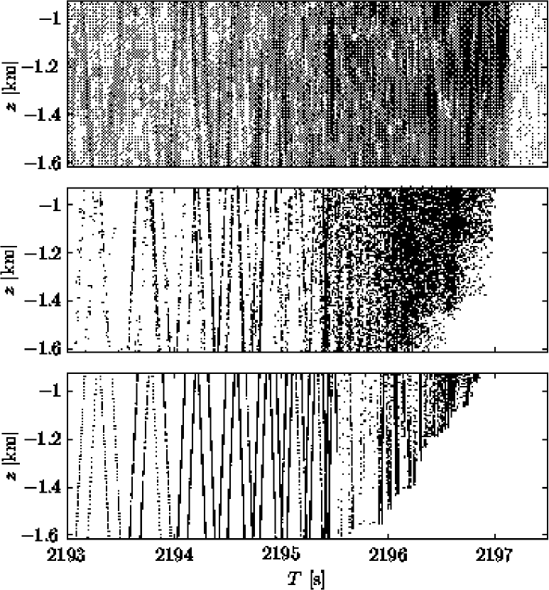
Figure 1: Measured and simulated AET wavefields in the time-depth plane. Upper panel: a typical measurement, shown on a gray scale plot with a dynamic range of 30 dB, of wavefield intensity. Middle panel: ray simulation with internal waves. Lower panel: ray simulation without internal waves. Wavefield intensity in the simulations is approximately proportional to the local density of dots, each corresponding to a ray.

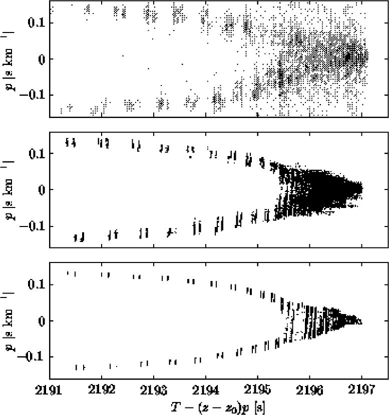
Figure 2: Same as Fig. 1 except that plane wave beamformed wavefields are shown. The beamformed ray simulations assume a dense receiving array whose upper and lower bounds coincide with the bounds of the AET receiving array. The reference depth was taken to be the depth of the uppermost hydrophone, $z_{o}=-0.9$ km.

Figure 1 shows a measured AET wavefield in the time-depth plane and ray-based simulations of such a wavefield with and without internal waves. Figure 2 is a complementary display that shows measured and simulated wavefields after plane wave beamforming. In this section we describe the most important qualitative features of measured and simulated AET wavefields. We begin by reviewing fundamental ray theoretical results so that our ray simulations can be fully understood. Also, this material provides a foundation for some of the later discussion. We then briefly describe the AET environment and the signal processing steps that were performed to produce the measured wavefield shown in Fig. 1. Next, our treatment of internal-wave-induced sound speed perturbations is briefly described. Finally, we return to describing and comparing qualitative features of the measured and simulated wavefields.

Fixed-frequency (cw) acoustic wavefields satisfy the Helmholtz equation,

$$\nabla^{2}u+\sigma^{2}c^{-2}(z,r)u=0,$$ (1)

where $\sigma=2\pi f$ is the angular frequency of the wavefield and $c(z,r)$ is the sound speed. (The extension to transient wavefields is straightforward using Fourier synthesis. It is not necessary to consider this complication to present the most important results needed below.) We assume propagation in the vertical plane with cartesian coordinates $z$ and $r$ representing depth and range, respectively. Ray methods can be introduced when the wavelength $2\pi c/\sigma$ of all waves of interest is small compared to the length scales that characterize variations in $c$. Substituting the geometric ansatz,

$$u(z,r;\sigma)=\sum_{j}A_{j}(z,r)e^{i\sigma T_{j}(z,r)},$$ (2)

representing a sum of locally plane waves, into the Helmholtz equation gives, after collecting terms in descending powers of $\sigma$, the eikonal equation,

$$(\nabla T)^{2}=c^{-2},$$ (3)

and the transport equation,

$$\nabla(A^{2}\nabla T)=0.$$ (4)

For notational simplicity, the subscripts on $A$ and $T$ have been dropped in (3) and (4).

The solution to the eikonal equation (3) can be reduced to solving a set of ray equations. If a one-way formulation (see, e.g., Ref. rdoa ) is invoked, with $r$ playing the role of the independent variable, the ray equations are

$$\frac{dz}{dr}=\frac{\partial H}{\partial p},\;\frac{dp}{dr}=-\frac{\partial H}{\partial z},$$ (5)

and

$$\frac{dT}{dr}=L=p\frac{dz}{dr}-H,$$ (6)

where

$$H(p,z,r)=-\sqrt{c^{-2}(z,r)-p^{2}}.$$ (7)

These equations constitute a nonautonomous Hamiltonian system with one degree of freedom; $z$ and $p$ are canonically conjugate position and momentum variables, $r$ is the time-like variable, $H$ is the Hamiltonian and the travel time $T$ corresponds to the classical action. Note also that $p\equiv p_{z}=\partial T/\partial z$ and $p_{r}=\partial T/\partial r=-H$ are the $z$- and $r$-components, respectively, of the ray slowness vector. The ray angle relative to the horizontal $\varphi$ satisfies $dz/dr=\tan\varphi$, or, equivalently, $cp=\sin\varphi$. For a point source rays can be labeled by their initial slowness $p_{0}$. The solution to the ray equations is then $z(r;p_{0})$, $p(r;p_{0})$, $T(r;p_{0})$. The terms in (2) correspond to eigenrays; these satisfy $z(r_{R};p_{0})=z_{R}$ where the depth and range of the receiver are $z_{R}$ and $r_{R}$, respectively. The transport equation (4) can be reduced to a statement of constancy of energy flux in ray tubes. The solution, for the $j$-th eigenray, can be written

$$A_{j}(z,r)=A_{0}\>|H/q_{21}|_{j}^{1/2}\>e^{-i\mu_{j}\frac{\pi}{2}}$$ (8)

where $H$, the matrix element $q_{21}$ and the Maslov index $\mu$ are evaluated at the endpoint of the ray, and $A_{0}$ is a constant. The stability matrix

$$Q=\left(\begin{array}[]{cc}q_{11}&q_{12}\\ q_{21}&q_{22}\end{array}\right)=\left(\begin{array}[]{cc}\left.\frac{\partial p}{\partial p_{0}}\right|_{z_{0}}&\left.\frac{\partial p}{\partial z_{0}}\right|_{p_{0}}\\ \left.\frac{\partial z}{\partial p_{0}}\right|_{z_{0}}&\left.\frac{\partial z}{\partial z_{0}}\right|_{p_{0}}\end{array}\right)$$ (9)

quantifies ray spreading,

$$\left(\begin{array}[]{c}\delta p\\ \delta z\end{array}\right)=Q\left(\begin{array}[]{c}\delta p_{0}\\ \delta z_{0}\end{array}\right).$$ (10)

Elements of this matrix evolve according to

$$\frac{d}{dr}Q=KQ$$ (11)

where $Q$ at $r=0$ is the identity matrix, and

$$K=\left(\begin{array}[]{cc}-{\partial^{2}H\over\partial z\partial p}&-{\partial^{2}H\over\partial z^{2}}\\ {\partial^{2}H\over\partial p^{2}}&{\partial^{2}H\over\partial z\partial p}\end{array}\right).$$ (12)

At caustics $q_{21}$ vanishes and, for waves propagating in two space dimensions, the Maslov index advances by one unit.

In ocean environments with realistic range-dependence, including the AET environment, ray trajectories are predominantly chaotic. Chaotic rays diverge from neighboring rays at an exponential rate, on average, and are characterized by a positive Lyapunov exponent,

$$\nu_{L}=\begin{array}[]{c}\lim\\ r\!\rightarrow\!\infty\end{array}\left(\frac{1}{r}\begin{array}[]{c}\lim\\ {\cal D}(0)\!\rightarrow\!0\end{array}\ln\frac{{\cal D}(r)}{{\cal D}(0)}\right).$$ (13)

Here ${\cal D}(r)$ is a measure of the separation between rays at range $r$; suitable choices for ${\cal D}$ are any of the four matrix elements of $Q$ or the trace of $Q$. The chaotic motion of ray trajectories leads to some limitations on predictability. This will be discussed in more detail below. Additional background material relating to this topic can be found in SVZ ; rdoa and references therein.

We digress now to briefly describe the AET experiment and relevant signal processing. In this experiment a source, suspended at 652 m depth from the floating instrument platform R/P FLIP in deep water west of San Diego, transmitted sequences of a phase-coded signal whose autocorrelation is pulse-like (with a pulse width of approximately 27 ms). The source center frequency was 75 Hz and the bandwidth was approximately 37.5 Hz. The resulting acoustic signals were recorded east of Hawaii at a range of 3252.38 km on a moored 20 element receiving array between the depths of 900 m and 1600 m. After correcting for the motion of the source and receiving array, including removal of associated Doppler shifts, the received acoustic signals were cross-correlated with a replica of the transmitted signal (to achieve the desired pulse compression) and complex demodulated. To improve the signal-to-noise ratio, 28 consecutive processed receptions, extending over a total duration of 12.7 minutes, were coherently added. The duration over which this coherent processing yields improved signal-to-noise is limited by ocean fluctuations, mostly due to internal waves. The statistics of the acoustic fluctuations were shown in Ref. CDT not to be adversely affected by the 12.7 minute coherent integration. Nearly concurrent with the week-long experiment, temperature profiles in the upper 700 m were measured with XBT’s every 30 km along the transmission path. An objective mapping technique was applied AET1 to these measurements to produce a map of the background sound speed structure (including mesoscale structure) along the transmission path. The sampling interval in range of the resulting sound speed field is 30 km so that no structure with horizontal wavelengths less than 60 km is present in this field. More details on the AET experiment, environment and processing of the acoustic signals can be found in Ref. AET1 .

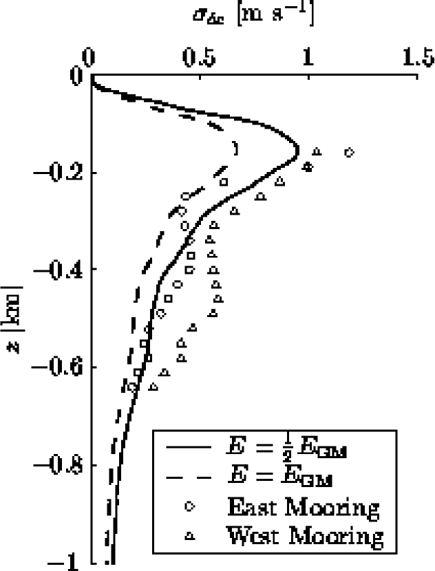
Figure 3: Measured and simulated rms sound speed fluctuations in the AET environment. The measurements shown were made near the source (labelled east) and near the receiving array (labelled west). The simulated fluctuations are due to internal waves using both $E=0.5\>E_{GM}$ and $E=1.0\>E_{GM}$, as described in the text.

Internal-wave-induced sound speed perturbations are taken into account in most of our simulations. These are assumed to satisfy the relationship $\delta c=(\partial c/\partial z)_{p}\zeta$ and the statistics of $\zeta$, the internal-wave-induced vertical displacement of a water parcel, were assumed to be described by the empirical Garrett-Munk spectrum (see, e.g., Ref. Miw ). The potential sound speed gradient $(\partial c/\partial z)_{p}$, the buoyancy frequency $N$, and the sound speed $c$ were estimated directly from hydrographic measurements using a procedure similar to that described in the appendix of Ref. WS ; it was found that a good approximation for the AET environment is $(\partial c/\partial z)_{p}/c\approx(1.25\;{\rm s}^{2}/{\rm m})N^{2}$. The vertical displacement $\zeta(r,z)$ was computed using equation 19 of Ref. CB with the variable $x$ replaced by $r$, and $y=t=0$. Physically this corresponds to a frozen vertical slice of the internal wave field that includes the influence of transversely propagating internal wave modes. A Fourier method, with $\Delta k_{x}=2\pi/3276.8$ km and $0<k_{x}\leq 2\pi/1$ km, was used to numerically generate sound speed perturbation fields. (Ray calculations were also performed using an internal wave field in which the hard upper bound on $k_{x}$ was replaced by an exponential damping of the large $k_{x}$ energy. The qualitative ray behavior described below did not depend on the manner in which the large $k_{x}$ cut-off was treated.) A mode number cut-off of $j_{max}=30$ was used in all the simulations shown. Contributions from approximately $2^{30}$ ($2^{15}/5\times 2^{15}/5\times 30$ where the factors of $1/5$ are present because the assumed wavenumber cut-off was one-fifth of the assumed Nyquist wavenumber) internal wave modes were included in our simulated internal-wave-induced sound speed perturbation fields. Measurements of sound speed variance made during the experiment (see Fig. 3) indicate that the internal wave energy strength parameter $E$ was close to $E_{GM}$, the nominal Garrett-Munk value. Simulations were performed using both $E=0.5\>E_{GM}$ and $E=1.0\>E_{GM}$. All of the simulations shown in this paper use $E=0.5\>E_{GM}$. The difference between these simulations and those performed using $E=1.0\>E_{GM}$ will be discussed where appropriate.

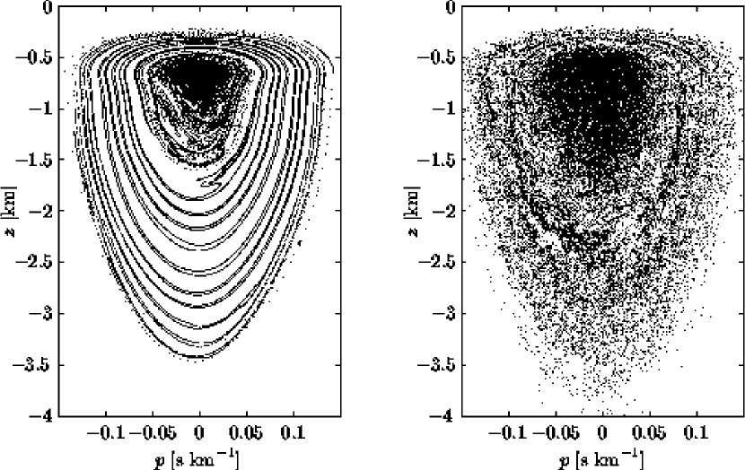
Figure 4: Simulated Lagrangian manifolds in the AET environment without (left panel) and with (right panel) internal waves. The ray density used in the plot on the right and for small $|p|$ in the plot on the left is too sparse to resolve what should, in each plot, be a smooth unbroken curve that does not intersect itself.

With the foregoing discussion as background, we are prepared to discuss our ray simulations in the AET environment. These are shown in Figs. 1, 2, 4 through 11, and 14. The points plotted in Figs. 1, 2 and 4 were computed by integrating the coupled ray equations (5, 6) from the source to the range of the receiving array. Several fixed and variable step-size integration algorithms were tested. In the presence of internal waves, convergence using a fixed step fourth order Runge Kutta integrator required that the step size not exceed approximately one meter. All ray tracing calculations presented in this paper were performed using double precision arithmetic (64 bit floating point wordsize). The wavefield intensity is approximately proportional to the density of rays (dots) that are plotted in Figs. 1 and 2. A somewhat more difficult calculation in which the contributions to the wavefield from many rays are coherently added will be discussed below.

In the presence of internal waves, rays with launch angles between approximately $\pm 5^{o}$ form the diffuse finale region of the arrival pattern arriving after approximately 2196 sec. Steeper rays contribute to the earlier, mostly resolved arrivals. It is seen in Fig. 1 that our ray simulation in the presence of internal waves underestimates the vertical spread of the finale region. Simulations with a stronger internal wave field, $E=1.0\>E_{GM}$, give a better fit to the vertical spread of energy (but a poorer fit to other wavefield features, as described below). Note, however, that diffractive effects, missing in our ray simulations, will contribute to enhanced broadening in depth of the arrival pattern. A striking feature of Figs. 1, 2 and 4 is the contrast between the seemingly structureless distribution of steep (large $|p|$) rays in $(p,z)$ seen in Fig. 4 when internal waves are present and the relatively structured distribution of the same rays in the time-depth (Fig. 1) and time-angle (Fig. 2) plots.

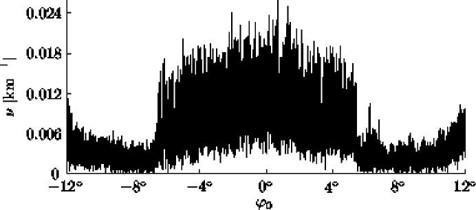
Figure 5: Stability exponents (finite range estimates of Lyapunov exponents) as a function of ray launch angle in the AET environment.

The cause of the complexity seen in Fig. 4 is ray chaos SVZ ; rdoa ; most ray trajectories diverge from initially infinitesimally perturbed rays at an exponential rate. 48,000 rays with launch angles between $\pm 12^{o}$ were traced to produce Figs. 1, 2 and 4 in the presence of internal waves. This fan of rays is far too sparse to resolve what should be an unbroken smooth curve – a Lagrangian manifold – which does not intersect itself in phase space (Fig. 4). Under chaotic conditions the separation between neighboring rays grows exponentially, on average, in range. The complexity of the Lagrangian manifold grows at the same exponential rate. The Lyapunov exponent is the recriprocal of the e-folding distance (see, e.g., rdoa ). Finite range numerical estimates of Lyapunov exponents (hereafter referred to as stability exponents) are shown as a function of launch angle in Fig. 5. It is seen that in this environment the flat rays ($|\varphi_{0}|\stackrel{{\scriptstyle<}}{{\scriptstyle\sim}}5^{o}$) have stability exponents of approximately 1/(100 km), while the steeper rays ($6^{o}\stackrel{{\scriptstyle<}}{{\scriptstyle\sim}}|\varphi_{0}|\stackrel{{\scriptstyle<}}{{\scriptstyle\sim}}11^{o}$) have stability exponents of approximately 1/(300 km). It follows, for example, that the complexity of the flat ray portion of the Lagrangian manifold grows approximately like $\exp(r/100\;{\rm km})$.

Not surprisingly, stability exponents show some sensitivity to parameters that describe the internal wave field. Our simulations show that the stability exponents of rays with axial angles of approximately $5^{o}$ or less approximately double when $j_{max}$ increases from 30 to 100, while steeper rays show very little sensitivity to $j_{max}$. In contrast, stability exponents of rays with axial angles from approximately $8^{o}$ to $15^{o}$ approximately double when $k_{max}$ increases from $2\pi/1000$ m to $2\pi/250$ m, while the flatter rays show little sensitivity to $k_{max}$. With these comments in mind, one should not attach too much significance to the details of Fig. 5. We note, however, that rays with axial angles of approximately $5^{o}$ or less consistently have higher stability exponents than rays in the $5^{o}$ to $10^{o}$ band.

Note that what appears to be temporally resolved arrivals in the measured wavefield correspond in our simulations to contributions from an exponentially large number of ray paths. (Only a small fraction of the total number are included in our simulations, however, because of the relative sparseness of our initial set of rays.) The observation that the travel times of chaotic ray paths may cluster and be relatively stable was first made in Ref. PGJ .

Simmen et al. SFW have previously produced plots similar to our Figs. 1 and 4 for ray motion in a deep ocean model consisting of a background sound speed structure very similar to ours on which internal-wave-induced sound speed perturbations were superimposed. Although our results are similar in many respects, it is noteworthy that the right panel of our Fig. 4 shows more chaotic behavior than is present in the corresponding plot in Ref. SFW . This difference persists if our 3252.38 km range simulations are replaced by simulations at the same range (1000 km) that was used in Ref. SFW . Our rays, especially the steeper rays, are more chaotic than those in Ref. SFW . We believe that this difference is primarily due to the increased complexity of our internal wave field over that of Simmen et al. SFW who included contributions from ten internal wave modes in their simulated internal wave fields.

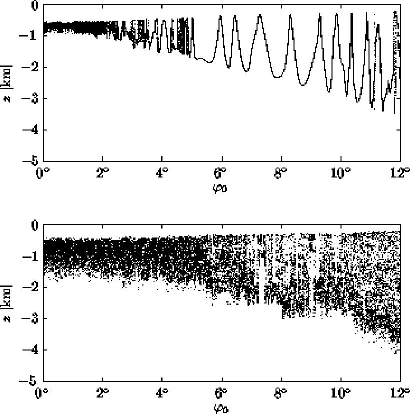
Figure 6: Ray depth vs. launch angle in the AET environment without (upper panel) and with (lower panel) internal waves. In both panels $\Delta\varphi_{o}=0.0005^{o}$.

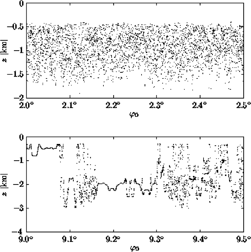
Figure 7: Ray depth vs. launch angle in two small angular bands in the AET environment with internal waves. In both panels $\Delta\varphi_{o}=0.000125^{o}$.

Figures 6 and 7 show plots of ray depth at the AET range vs. launch angle. In Fig. 6 the same rays (excluding those with negative launch angles) that were used to produce Figs. 1, 2 and 4 are plotted. In Fig. 7 two small angular bands of the upper panel of Fig. 6 are blown up; the ray density is four times greater than that used in Fig. 6. Fig. 6 strongly suggests that, even in the absence of internal waves, the near-axial rays are chaotic. Not surprisingly, in the presence of internal waves, steeper rays are also predominantly chaotic. Note, however, that Figs. 5, 6 and 7 show that the near-axial rays are evidently more chaotic than the steeper rays. An explanation for this difference in behavior will be given in section III.

In this section we have briefly described and compared the gross features of measured and simulated AET wavefields. Ray trajectories in our simulated wavefields in the presence of internal waves are predominantly chaotic. In spite of this, Figs. 1 and 2 show that many features of our simulated wavefields are stable and in good qualitative agreement with the observations. Predicted and measured spreads of acoustic energy in time, depth and angle are generally in good agreement, both in the early and late portions of the arrival pattern. We shall not discuss further the spreads of energy in depth and angle, except to note that Figs. 1 and 2 show that these spreads can be accounted for using ray methods in the presence of realistic (including internal-wave-induced sound speed perturbations) ocean structure. In the two sections that follow we shall consider in more detail the time spreads of the early ray arrivals, and intensity statistics in both the early and late portions of the arrival pattern.

III Chaos, micromultipaths and timefront stability

In this section we consider in some detail eigenrays, timefront stability and time spreads. We focus our attention on the early branches of the timefront, where measured time spreads were, surprisingly, only approximately 2 ms, in sharp contrast to the theoretical prediction of approximately 1 sec AET2 . We focus our attention on the early arrival time spreads, primarily because quantitative estimates of the unresolved late arrivals are not available.

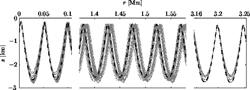
Figure 8: Three segments of the range-depth plane along the AET transmission path showing a subset of a set of micromultipaths. The three rays that have the strongest amplitudes are shown using dashed lines; these rays are not resolved on this plot.

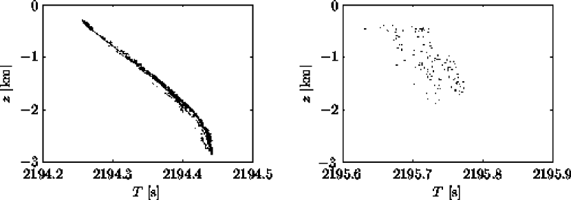
Figure 9: Ray depth vs. travel time in the AET environment with internal waves, but only for rays with identifiers $+137$ (left panel) and $+151$ (right panel). The points plotted are a subset of those plotted in the lower panel of Fig. 1.

Eigenrays at a fixed depth $z$ correspond to the intersections of a horizontal line at depth $z$ with the curve $z(\varphi_{o})$; these intersections are the roots of the equation $z-z(\varphi_{o})=0$. Although the discrete samples of $z(\varphi_{o})$ plotted in Figs. 6 and 7 are too sparse to reveal what should be a smooth curve, it is evident the number of eigenrays at almost all depths is very large; because rays are predominantly chaotic, this number grows exponentially in range. In principle, eigenrays can be found using a combination of interpolation and iteration, starting with a set of discrete samples of $z(\varphi_{o})$. In practice, this procedure reliably finds only those eigenrays in regions where $z(\varphi_{o})$ has relatively little structure. These rays have the highest intensity and are the least chaotic. It is seen in Fig. 1 that the early (steeper) ray arrivals come in clusters with small travel time spreads. The set of eigenrays within such a cluster is often referred to as a set of micromultipaths. An incomplete set of micromultipaths, found using the procedure just described, is shown in Fig. 8. An interesting and important feature of micromultipaths in our simulations is that all of the rays that make up a set of micromultipaths have the same identifier $\pm M$. Here $\pm$ is the sign of the launch angle and $M$ is the number of ray turning points (where $p$ changes sign) following a ray. In Fig. 9 rays with two fixed values of ray identifier (+137 and +151) are plotted in the time-depth plane. In both cases the points plotted are a subset of those plotted in Fig. 1. It is seen that the relatively steep +137 rays have a small time spread and form one of the branches of the timefront seen in Fig. 1 (similar behavior was noted in Ref. SFW ), while the relatively flat +151 rays have a much larger time spread and fall within the diffuse finale region of the arrival pattern seen in Fig. 1.

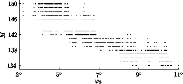
Figure 10: Ray identifier vs. launch angle for a subset of the rays that are plotted in Fig. 6.

An important (and surprising) feature of sets of micromultipaths is that they are highly nonlocal in the sense that interspersed (i.e., having intermediate launch angles) among a group of micromultipaths are rays with $M$ values that differ by several units. This behavior is illustrated in Fig. 10. In view of the observation that, in the presence of internal waves in the AET environment, ray motion is strongly chaotic and the function $M(\varphi_{o})$ has local oscillations of several units, it is remarkable that the early portion of the timefront (see Fig. 1) is not destroyed. The nonlocality of a set of micromultipaths in the range-depth plane is seen in Fig. 8. Note that there are significant differences in the upper and lower turning depths of the plotted micromultipaths and that these rays are spread in range by a significant fraction of a ray cycle distance.

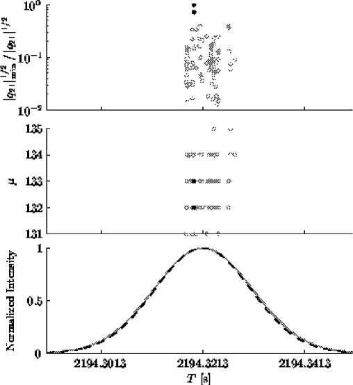
Figure 11: Upper panel: normalized ray intensity vs. travel time for a subset of the eigenrays (micromultipaths) with identifier +137 that connect the AET source and a receiver at depth 1005 m at the AET range. Middle panel: the corresponding Maslov indices vs. travel time. Lower panel: envelope of the waveform synthesized by coherently adding the contributions from all the micromultipaths shown (solid curve), and the normalized envelope of the AET source waveform (as seen in the far field; dashed line). The three rays whose intensity is largest are shown using solid circles in the upper and middle panels; the remaining rays are shown using open circles.

The result of performing a ray-based synthesis of what appears in the measurements to be an isolated arrival is shown in Fig. 11. This involves finding a complete set of micromultipaths, including their travel times and Maslov indices, and coherently summing their contributions. Unfortunately, owing to the predominantly chaotic motion of ray trajectories in the AET environment in the presence of internal waves, it is extremely difficult to find a complete set of micromultipaths. Indeed, the constituent ray arrivals used in the Fig. 11 synthesis do not constitute a complete set of micromultipaths. This is less important than might be expected because standard eigenray finding techniques easily locate the strongest micromultipaths; the missing micromultipaths in the Fig. 11 synthesis are highly chaotic rays that have very small amplitudes. An interesting result of this synthesis is that the micromultipath-induced time spread in the synthesized pulse is only about 1 ms, which is in very good agreement with the AET measurements AET2 ; CDT . Note that the total time spread among the micromultipaths found – about 11 ms – is much greater than the spread of the synthesized pulse. This difference arises because the time spread of the dominant micromultipaths is much smaller than the total micromultipath time spread.

Simulations (not shown) using $E=1.0\>E_{GM}$ result in synthesized steep ray pulses that are spread in time much more than is shown in Fig. 11. With the stronger internal wave field, the total micromultipath time spread increases by approximately a factor of two – to about 25 ms. More importantly, however, the dominant micromultipaths have time spreads comparable to the total micromultipath time spread, leading to synthesized pulses that are spread by 5 to 10 ms, rather than 1 to 2 ms. Thus, measured early arrival time spreads are in better agreement with $E=0.5\>E_{GM}$ simulations than with $E=1.0\>E_{GM}$ simulations. The question of which value of the internal wave strength $E$ in our simulations gives the best fit to the observations will be revisited in the next section.

An interesting and unexpected feature of our simulations is that the Maslov index was consistently lower than the number of turns $M$ made by the same ray. The difference was typically three units in the $E=0.5\>E_{GM}$ simulations and four units in the $E=1.0\>E_{GM}$ simulations. We have no explanation for this behavior.

So far in this section we have seen that associated with the chaotic motion of ray trajectories is extensive micromultipathing, and that the micromultipathing process is highly nonlocal. The many micromultipaths that add at the receiver to produce what appears to be a single arrival may sample the ocean very differently. Surprisingly, on the early arrival branches the highly nonlocal micromultipathing process causes only very small time spreads and does not lead to a mixing of ray identifiers. To complete this picture it is necessary to explain why the time spreads of the early (steep) ray arrivals are so small. We shall now provide such an explanation. Recall first, however, that the measured time spread of the early arrivals is only approximately 2 ms AET2 , in marked contrast to the theoretical prediction FDMWZ ; AET2 of approximately 1 sec. Thus our quantitative explanation for the small early arrival time spreads serves both to give insight into the underlying physics, and provides an explanation for a critically importnat feature of the measured AET wavefields.

Computing time spreads is conceptually straightforward using ray methods. In a known environment one finds a large ensemble of rays with the same identifier that solve the same two point boundary value problem; the spread in travel times over many ensembles of such rays, each ensemble computed using in a different realization of the environment, is the desired quantity. The constraint that all of the computed rays have the same fixed endpoints complicates this calculation. In the following we exploit an approximate form of the eigenray constraint that simplifies the calculation; the approximate form of the eigenray constraint is first order accurate in a sense to be described below.

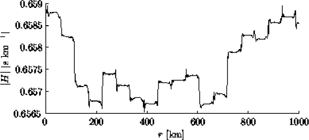
Figure 12: $|H|$ vs. range following a ray emitted on the sound channel axis with a launch angle of $11^{o}$ in a canonical environment with an internal-wave-induced sound speed perturbation superimposed.

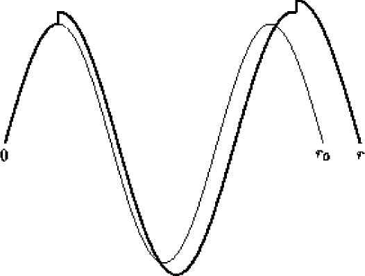
Figure 13: Schematic diagram showing a twice apex-scattered ray (heavy line) and the path that the same ray would have followed in the absence of apex scattering events (light line).

Before describing the manner in which the eigenray constraint is imposed, it is useful to describe the physical setting in which the constraint will be applied. Figure 12 shows $|H|$ vs $r$ following a moderately steep ray (axial angle approximately $11^{o}$) in a canonical environment Mcan on which the previously described (based on the measured AET $N(z)$ profile) internal-wave-induced sound speed perturbation field was superimposed. It is seen that $H(r)$ consists of a sequence of essentially constant $H$ segments, separated by near-step-like jumps. The jumps occur at the ray’s upper turning points. A simple model that captures this behavior – the so-called apex approximation FDMWZ – assumes that the transition regions can be approximated as step functions. (The validity of the apex approximation is linked to the anisotropy and inhomogeneity of oceanic internal waves; details of the background sound speed profile are not important. For this reason we have chosen to illustrate this effect using a background canonical profile rather than the AET environment.) Figure 13 shows a schematic diagram of two rays. One ray has undergone two internal-wave-induced apex scattering events; the other ray is an unscattered ray with the same launch angle as the scattered ray.

Our strategy to building the eigenray constraint into an estimate of travel time spreads can now be stated. We consider a scattered and an unperturbed (that is, in the absence of internal-wave-induced scattering events) ray with the same ray identifier; the rays shown schematically in Fig. 13 have identifier $+3$. In addition to having the same ray identifier, the scattered and unperturbed rays are assumed to start from the same point and end at the same depth, but they will generally end at different ranges. We assume that the scattered ray has travel time $T_{r}$ and is one of many scattered eigenrays with the same ray identifier at range $r$. We estimate the travel time $T(r)$ of an unperturbed eigenray at range $r$ whose ray identifier is the same as that of the scattered eigenray. It will be shown that $\delta T(r)=T_{r}-T(r)$ vanishes to first order if the apex approximation is exploited. Because the same result applies to all of the scattered eigenrays, it follows that the time spread vanishes to first order, independent of $r$, if the apex approximation is exploited. Note that this result is not expected to apply, even approximately, to the late near-axial rays where the apex approximation is known to fail.

The travel time $T(r)$ of the eigenray in the unperturbed ocean can, of course, be computed numerically but this provides little help in deriving an analytical estimate of $\delta T$. Instead, consider a ray in the unperturbed ocean with the same launch angle as one of the scattered eigenrays, as shown in Fig. 13. In general, the range of this ray at the receiver depth, after making the appropriate number of turns, will be $r_{o}\neq r$. But $T(r)$ can be estimated from $T(r_{o})$. This follows from the observation that ray travel time (assuming a point source initial condition, for instance) is a continuously differentible function of $z$ and $r$ with $\nabla T=\bf{p}$ where $\bf{p}$ is the ray slowness vector. Because of this property $T(z,r)$ can be expanded in a Taylor series. If we consider rays with the same ray identifier and fix the final ray depth to coincide with the receiver depth, then

$$T(r)\approx T(r_{o})+p_{r}(r_{o})(r-r_{o})$$ (14)

where $p_{r}=-H$ is the $r$-component of the ray slowness vector. (More generally, $T(z,r)$ consists of multiple smooth sheets that are joined at cusped ridges; in spite of this complication, the property of continuous differentiability is maintained, even in a highly structured ocean. For our purposes, we need only consider one sheet of this multi-valued function. Note also that our application of (14) in the background ocean makes this expression particularly simple to use.) It follows from (14) that

$$\delta T(r)=T_{r}-T(r)\approx T_{r}-T(r_{o})-p_{r}(r_{o})(r-r_{o})$$ (15)

is, correct to first order, the travel time difference at range $r$ between eigenrays with and without internal waves.

To evaluate $\delta T(r)$ we shall assume that the backgound environment is range-independent. Also, consistent with the use of the apex approximation, we may treat the perturbed environment as piecewise range-independent. Within each range-independent segment it is advantageous to make use of the action-angle variable formalism (see. e.g., rdoa or AV01 ). In terms of the action-angle variables $(I,\theta)$, $\tilde{H}=\tilde{H}(I)$ and the ray equations are

$$\frac{d\theta}{dr}=\frac{\partial\tilde{H}}{\partial I}=\omega(I),$$ (16)

$$\frac{dI}{dr}=-\frac{\partial\tilde{H}}{\partial\theta}=0,$$ (17)

and

$$\frac{dT}{dr}=I\frac{d\theta}{dr}-\tilde{H}(I)=I\omega(I)-\tilde{H}(I),$$ (18)

where the physical interpretation of $\tilde{H}$ as $-p_{r}$ is maintained. The angle variable can be defined to be zero at the upper turning depth of a ray and increases by $2\pi$ over a ray cycle (double loop). It follows that the frequency $\omega(I)=2\pi/R(I)$ where $R(I)$ is a ray cycle distance. Integrating the ray equations over a complete ray cycle then gives $R(I)=2\pi/\omega(I)$ and $T(I)=2\pi(I-\tilde{H}(I)/\omega(I))$ with $I$ constant following each ray. In the apex approximation $I$ jumps discontinuously at each ray’s upper turning depth; for the perturbed ray $R(I+\Delta I)\approx 2\pi/\omega(I)-2\pi\Delta I\omega^{\prime}(I)/(\omega(I))^{2}$ and $T(I+\Delta I)\approx 2\pi(I-\tilde{H}(I)/\omega(I))+2\pi\Delta I\tilde{H}(I)\omega^{\prime}(I)/(\omega(I))^{2}$ where $\omega^{\prime}(I)=d\omega(I)/dI$. Note that, like these expressions, Eqs. 14 and 15 are first order accurate in $\Delta I$.

Consider again Eq. 15 and Fig. 13 with $I$ equal to $I_{0}$, $I_{1}$ and $I_{2}$ in the left center and right ray segments, respectively. The left segment gives no contribution to $\delta T$ as the ray has not yet been perturbed. In the center ray segment

$$T_{r}-T(r_{o})\approx 2\pi(I_{1}-I_{0})\frac{\tilde{H}(I_{0})\omega^{\prime}(I_{0})}{(\omega(I_{0}))^{2}}$$ (19)

and

$$-p_{r}(r_{o})(r-r_{o})\approx\tilde{H}(I_{0})\left[-2\pi(I_{1}-I_{0})\frac{\omega^{\prime}(I_{0})}{(\omega(I_{0}))^{2}}\right].$$ (20)

These terms are seen to cancel. Note that if additional complete cycle ray segments are added to the center section of the ray, Eqs. 19 and 20 are unchanged except that $I_{1}-I_{0}=\Delta I_{1}$ is replaced by $\sum_{i=1}^{n}\Delta I_{i}=I_{n}-I_{0}$; again the two terms cancel. In the final (incomplete cycle) ray segment the difference between the terms $T_{r}-T(r_{o})$ and $p_{r}(r_{o})(r-r_{o})$ can be shown to be $O((\Delta I)^{2})$; the terms do not exactly cancel because the $\theta$-values of the perturbed and unperturbed rays are generally not identical at the receiver depth. Thus, to first order in $\Delta I$, $\delta T=0$, independent of range, if the apex approximation is valid. This simple calculation provides an explanation of why, in spite of extensive ray chaos, the time spreads of the early AET ray arrivals are quite small.

Several comments concerning the preceeding calculation are noteworthy. First, we note that although it was assumed that the background sound speed structure is range-independent, the preceeding argument also holds in the presence of slow background range-dependence, i.e., with structure whose horizontal scales are large relative to a typical ray double loop length. Adiabatic invariance in such environments guarantees that while $H$ is not constant following rays between apex scattering events, $I$ is nearly constant. Second, after $n$ random kicks $I_{1}-I_{0}$ in (19) and (20) is replaced by $I_{n}-I_{0}\approx\sqrt{n}(\Delta I)_{rms}$, and the magnitude of (19) under AET conditions is $O(1\;\rm{sec})$. This is an example of a travel time spread estimate that fails to enforce the eigenray constraint. This calculation shows that the difference between travel time estimates that do and do not enforce the eigenray constraint can be quite significant. (The constrained estimate is refined below.) Third, it should be emphasized that Eqs. (19) and (20) apply (approximately) only to the steep rays because the apex approximation applies only to the steep rays. We have not addressed the time spreads of near-axial rays. Note, however, that Fig. 9 shows that time spreads are larger for flatter rays. Fourth, the above calculation shows that, to lowest order in $\Delta I$, there is no internal-wave-scattering-induced travel time bias if the apex approximation is strictly applied. And fifth, the arguments leading to Eqs. (19) and (20) apply whether the scattered rays are chaotic or not.

A relaxed form of the apex approximation in which the action jump transition region has width $\Delta\theta$ gives a nonzero travel time spread estimate. In the transition region, taken for convenience to be $0\leq\theta\leq\Delta\theta$, one may choose a Hamiltonian of the form $\tilde{H}=\tilde{H}(I-s\theta)$ where $s=\Delta I/\Delta\theta$, and $\tilde{H}=\tilde{H}(I)$ elsewhere. It follows that in the transition region $I(\theta)=I_{0}+s\theta$ and $I=\rm{constant}$ elsewhere. A simple generalization of the above calculation then gives for a complete ray cycle

$$T_{r}-T(r_{o})\approx$$ (21)

$$\!\!\!\!\!\!\!\!\!\!\!\!\!\!\!\!\!\!\!\!\!\!\!\!\!\!\!\!\!\!(I_{1}-I_{0})\left[(2\pi-\Delta\theta)\frac{\tilde{H}(I_{0})\omega^{\prime}(I_{0})}{(\omega(I_{0}))^{2}}+\frac{\Delta\theta}{2}\right]$$

and

$$-p_{r}(r_{o})(r-r_{o})\approx$$ (22)

$$\!\!\!\!\!\!\!\!\!\!\!\!\!\!\!\!\!\!\!\!\!\!\!\!\!\!\!\!\!\!\tilde{H}(I_{0})\left[-(2\pi-\Delta\theta)(I_{1}-I_{0})\frac{\omega^{\prime}(I_{0})}{\omega(I_{0})^{2}}\right],$$

so the sum (recall [15]) is

$$\delta T\approx\frac{\Delta\theta}{2}(I_{1}-I_{0}).\\$$ (23)

It should be emphasized that this expression is first order accurate in $\Delta I=I_{1}-I_{0}$, but that no assumption about the smallness of $\Delta\theta$ has been made. As noted above, incomplete cycle end segment pieces give $O((\Delta I)^{2})$ corrections to $\delta T$. If $\Delta\theta$ has approximately the same value at each upper turn, then one has after $n$ upper turns, correct to $O(\Delta I)$,

$$\delta T\approx\frac{\Delta\theta}{2}\sum_{i=1}^{n}(I_{i}-I_{i-1}) = \frac{\Delta\theta}{2}(I_{n}-I_{0})$$ (24)

$$\approx \frac{\Delta\theta}{2}\sqrt{n}(\Delta I)_{rms}.$$

Consistent with the numerical simulations shown in Fig. 12, $\Delta\theta\approx 0.8$ radians and $\Delta I\approx 4$ ms. (We, and independently F. Henyey [personal communication], have confirmed that these estimates also apply under AET-like conditons.) With these numbers and $\sqrt{n}=8$, appropriate for AET, (24) gives a time spread estimate of approximately 13 ms, in approximate agreement with the numerical simulations shown in Fig. 11. Note that (24) does not preclude a travel time bias. A cautionary remark concerning the use of (24) is that Virovlyansky XX has pointed out that, owing to secular growth, the $O((\Delta I)^{2})$ contribution to $\delta T$ may dominate the $O(\Delta I)$ contribution at long range.

Figure 9 shows that in the AET environment simulated near-axial ray time spreads are greater than simulated steep ray time spreads. We do not fully understand this behavior. A possible explanation for this behavior is that time spreads increase as rays become increasingly flat owing to the breakdown of the apex approximation. But one would expect that this trend should be offset, in part or whole, by the relative smallness of internal-wave-induced sound speed perturbations near the sound channel axis. In addition, we have seen some evidence that an additional factor may be important in the AET environment. Namely, we have observed a positive correlation between travel time spreads and stability exponents; stability exponents in the AET environment are shown in Fig. 5. We have chosen not to dwell on flat ray time spreads in this paper because there are no AET measurements of these spreads to which simulations can be compared. It is clear, however, that the issues just raised need to be better understood.

IV Wavefield intensity statistics

In this section we consider the statistical distribution of the intensities of both the early and late AET arrivals. Recall that experimentally the early arrival intensities have been shown AET2 ; CDT to approximately fit a lognormal probability density function (PDF) and the late arrival intensities have been shown CDT to fit an exponential distribution. The late arrival exponential distribution is not surprising as this distribution is characteristic of saturated statistics. The early arrival near-lognormal distribution is surprising, however, inasmuch as theory FDMWZ ; AET2 predicts saturated statistics, i.e., an exponential intensity PDF. It has been argued C99 that the theory can be modified in such a way as to move the early arrival prediction from saturated to unsaturated statistics. The latter regime is characterized by a lognormal intensity PDF. This fix is conceptually problematic inasmuch as, in this theory, the unsaturated regime is characterized by the absence of micromultipaths, which seriously conflicts with the numerical simulations presented in the previous section where the number of micromultipaths is very large. In this section we provide self-consistent explanations for both the late arrival exponential distribution and the early arrival lognormal distribution. The challenge is to reconcile the early arrival near-lognormal intensity PDF with the presence of a large number of micromultipaths. Some of the arguments presented are heuristic, and some build on the results of numerical simulations. A complete theoretical understanding of intensity statistics has proven difficult.

Our approach to describing wavefield intensity statistics builds on the semiclassical construction described by Eq. (2). At a fixed location it is seen that the wavefield amplitude distribution is determined by the distribution of ray amplitudes and their relative phases. Note that both travel times and Maslov indices influence the phases of ray arrivals. Complexities associated with transient wavefields and caustic corrections will be discussed below.

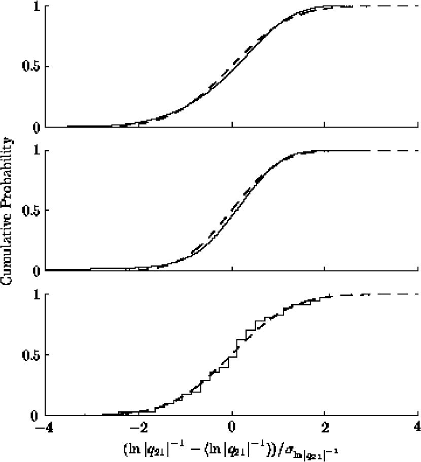
Figure 14: Cumulative probability density of ray intensity in the AET environment. Upper panel: flat rays ($|\varphi|\leq 5^{o}$) sampled uniformly in launch angle. Middle panel: steep rays ($6^{o}\leq|\varphi|\leq 11^{o}$) sampled uniformly in launch angle. Lower panel: eigenrays with $+137$ identifier connecting the AET source and a receiver at depth 1005 m at the AET range. In all three panels the dashed lines correspond to lognormal distributions whose mean and variance approximately match those of the simulations.

An important observation is that in the AET environment, including internal-wave-induced sound speed perturbations, simulated geometric amplitudes of both steep and flat ray arrivals approximately fit lognormal PDFs. This is shown in Fig. 14. Previously it has been shown WTo that ray intensities in a very different chaotic system also fit a lognormal PDF; in that system single scale isotropic fluctuations are superimposed on a homogeneous background. (Note that all powers of a lognormally distributed variable are also lognormally distributed, so ray amplitudes have this property if and only if ray intensities have this property.) The apparent generality of the near-lognormal ray intensity PDF suggests that it applies generally to ray systems that are far from integrable; the arguments presented in Ref. WTo suggest that this should be the case. The intensity distributions of the early and late AET arrivals, corresponding to steep and flat rays, respectively, will be discussed separately.

We consider first the early arrivals. We saw in the previous section that the micromultipaths that make up one of these arrivals have the same ray identifier and have a very small spread in travel time. The dominant micromultipaths were seen (see Fig. 11) to have a time spread of approximately 1 ms which is a small fraction of the approximately 13 ms period of the 75 Hz carrier wave. Also, our simulations show that the Maslov indices of the dominant micromultipaths differ by no more than one unit. These conditions dictate that interference among the dominant micromultipaths is predominantly constructive. Because travel time differences are so small, the pulse shape should have negligible influence on the distribution of peak intensities. In a model of the early AET arrivals consisting of a superposition of interfering micromultipaths, the micromultipath properties that play a critical role in controlling peak wavefield intensities are thus: 1) their amplitudes have a near-lognormal distribution; 2) the dominant micromultipaths have negligible travel time differences; and 3) the dominant micromultipaths have Maslov indices that differ by no more than one unit. It should be noted that very different behavior would have been observed if: the source bandwidth were significantly more narrow as this would have caused micromultipaths with different ray identifiers to interfere with one another; or the source center frequency were significantly higher as phase differences between interfering micromultipaths would then have been significant.

An additional subtlety must be introduced now: the PDF of the intensities of the constituent micromultipaths that make up a single arrival is not identical to the PDF described in Ref. WTo and shown in the upper and middle panels of Fig. 14. The latter PDF describes the distribution of intensities of randomly (with uniform probability) selected rays leaving the source within some small angular band and whose range is fixed. This PDF is biased in the sense that it overcounts the micromultipaths with large intensities and undercounts those with small intensities. Unbiased micromultipath intensity PDFs can be constructed from the biased PDFs shown. To do so, consider a manifold (a smooth curve in phase space corresponding to a fan of initial rays) which begins near $(z_{0},p_{0})$ and arrives in the neighborhood of $(z_{r},p_{r})$ at range $r$. Sampling in fixed steps of the differential $\delta p_{0}$ (as was done to produce the upper and middle panels of Fig. 14; this is equivalent to uniform random sampling) leads to a highly nonuniform density of points on the final manifold since $(z_{0},p_{0}+\delta p_{0})$ propagates to $(z_{r}+q_{21}\delta p_{0},p_{r}+q_{11}\delta p_{0})$. The greater $q_{21}$, the lower the density of points locally at final range. A uniform sampling in final position is acheived instead by considering the initial conditions that would lead to $(z_{r}+\delta z_{r},p_{r}+q_{11}/q_{21}\delta z_{r})$. Its density of points on the initial manifold can be deduced from its initial condition, $(z_{0},p_{0}+\delta z_{r}/q_{21})$. It is necessary to sample $q_{21}$ times more densely on the initial manifold in order to acheive uniform sampling in $\delta z_{r}$ at range $r$. To account for this effect, we need to know the PDF for $q_{21}$ with uniform initial sampling. Roughly speaking, the PDF of the absolute values of the individual matrix elements of $q$ have the same form as for $|Tr(Q)|$, apart from a shift of the centroid that is lower order in range than the leading term. From the results of Ref. WTo , the (biased in the sense described above) probability that $q_{21}$ falls in the interval between $x$ and $x+dx$ is

$$\rho_{|q_{21}|}(x)=\sqrt{\frac{1}{2\pi r(\bar{\nu}-\nu_{L})}}\frac{1}{x}\;\cdot\qquad$$ (25)

$$\!\!\!\!\!\!\!\!\!\!\!\!\!\!\!\!\!\!\!\!\!\!\!\!\!\!\!\!\!\!\!\!\!\!\!\!\!\!\!\!\!\!\!\!\!\!\!\!\!\!\!\!\!\!\!\!\!\!\!\!\exp{\left[\frac{-\left(\ln{(x)}-\nu_{L}r\right)^{2}}{2r(\bar{\nu}-\nu_{L})}\right]}\;,\;x\geq 0\;.$$

Here $\bar{\nu}$ is a finite-range estimate of the Lyapunov exponent based on an average (over an ensemble of rays) value of $q_{21}$, and $\nu_{L}$ is the true Lyapunov exponent. The new (unbiased in the sense described above) PDF, $\rho^{\prime}$, for uniform sampling in $\delta z_{r}$ is related to the previous one by

$$\rho^{\prime}_{|q_{21}|}(x) = \frac{x}{\langle x\rangle}\rho_{|q_{21}|}(x)$$ (26)

$$= \sqrt{\frac{1}{2\pi r(\bar{\nu}-\nu_{L})}}\frac{1}{x}\;\cdot$$

$$\exp{\left[\frac{-\left(\ln{(x)}-\bar{\nu}r\right)^{2}}{2r(\bar{\nu}-\nu_{L})}\right]}\;,\;x\geq 0$$

where the factor $x$ accounts for the extra counting weight of $q_{21}$, and $\langle x\rangle$ just preserves normalization and is calculated using Eq. (25). This calculation shows that the unbiased micromultipath ray intensity PDF also has a lognormal distribution; the only change relative to the biased PDF is an increase in the mean from $\nu_{L}r$ to $\bar{\nu}r$. Because lognormality is maintained, this correction represents only a trivial change to the problem.

Approximate lognormality of the constrained (eigenray) PDF of ray intensity is shown in the lower panel of Fig. 14. This PDF was constructed using the same eigenrays that were used to produce Figs. 8 and 11. The corresponding unconstrained ray intensity PDF is shown in the middle panel of Fig. 14. (Two constraints – fixed receiver depth and fixed ray identifier – are built into the lower panel PDF. A very similar constrained PDF results if only the receiver depth constraint is applied, provided ray launch angles are limited to the ‘steep’ ray band used to construct the middle panel.) It should be noted that the constrained (eigenray) PDF shown in the lower panel of Fig. 14 was constructed from numerically found eigenrays; because weak eigenrays are difficult to find numerically they are undercounted and the PDF is biased. In a practical sense this bias is of little consequence because the weak eigenrays that are difficult to find contribute negligibly to the wavefield.

We return now to the problem of simulating the early AET arrivals. It is tempting to think that because the constituent micromultipaths have a near-lognormal distribution, the sum of their contributions should also be near-lognormally distributed. Unfortunately, this is generally not the case. Consider, for example, the special case in which phase, including Maslov index, differences are negligible. Then all micromultipaths interfere constructively and peak wavefield amplitudes can be modelled as the sum of many lognormally distributed variables. Because all moments of the lognormal distribution are finite, the central limit theorem applies. Under these conditions, if sufficiently many contributions are summed, the distribution of the sums – the wavefield amplitudes – would be a gaussian.

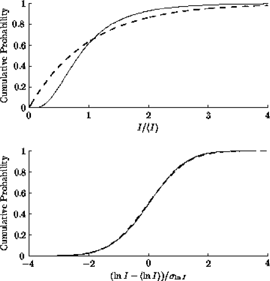
Figure 15: Cumulative probability density of peak wavefield intensity simulated using a simple model as described in the text. The same simulated cumulative density is compared to exponential (upper panel dashed line) and lognormal (lower panel dashed line) cumulative density functions. This figure should be compared to Fig. 14 in Ref. AET2 .

To simulate the statistics of the early AET arrivals (recall Fig. 14 and the accompanying discussion) we have used several variations of a simple model. An arrival was modelled as a sum of $n_{m}$ interfering micromultipaths whose: 1) amplitudes are lognormally distributed; and 2) phases, $\omega T_{i}-\mu_{i}\pi/2\bmod 2\pi$, have a clearly identifiable peak. Micromultipath contributions were coherently added. The peak intensity of the sum – whose travel time is not known a priori – was then recorded. Using an ensemble of $10^{4}$ peak intensities, a peak intensity PDF was then constructed. Peak intensity PDFs constructed in this fashion were found to be very close to lognormal; a typical example is shown in Fig. 15. In this example $f=\omega/2\pi=75$ Hz, the $T_{i}$’s were identical, $\mu_{i}\in{j,j+1}$ with equal probability (note that choice of the integer $j$ is unimportant) and $n_{m}=5$. Other combinations of distributions for $T_{i}$ (either a Gaussian or the limiting case of a delta distribution), $\mu_{i}$ (taken either from ${j,j+1}$ or ${j-1,j,j+1}$ with equal probability), and the parameter $n_{m}$ (between 2 and 100) were tested. These simulations showed that provided the phase constraint noted above was satisfied, a near log-normal peak intensity PDF resulted.

Two points regarding this simple model are noteworthy. First, this model does not constitute a theory of wavefield peak intensity statistics, but it does serve to demonstrate that our ray-based simulations of the early AET arrivals are consistent with the measured distribution of peak intensities. Second, simulations (not shown), performed with $E=1.0\>E_{GM}$ yield sets of dominant micromultipaths that violate assumption 2); phases are uniformly distributed and summing micromultipath contributions yields a distribution of peak intensities that is not close to lognormal. Thus, our simulations suggest that a near-lognormal distribution of early arrival peak intensity requires a relatively weak internal wave field.

A complication not accounted for in the preceeding discussion is the presence of caustics. At caustics geometric amplitudes (8) diverge and diffractive corrections must be applied. At short range (on the order of the first focal distance – a few tens of km in deep ocean environments) we expect that intensity fluctuations will be dominated by diffractive effects. The entire wavefield should be organized by certain high-order caustics which leads to a PDF of wavefield intensity with long tails twink ; twink2 ; twink3 . In spite of the importance of diffractive effects at short range – and probably also at very long range – we believe that, in the transitional regime described above, intensity fluctuations are not dominated by diffractive effects. This somewhat counterintuitive behavior can be understood by noting that in the vicinity of caustics the importance of diffractive corrections to (8) decreases as the curvature of the caustic increases. Under chaotic conditions the curvature of caustics increases, on average, with increasing range, so the fraction of the total number of multipaths that require caustic corrections decreases, on average, with increasing range. This is true even as the number of caustics grows exponentially, on average, in range. This argument leads to the somewhat paradoxical conclusion that, prior to saturation at least, we expect that the importance of caustic corrections decreases with increasing range.

We turn our attention now to the late unresolved AET arrivals, corresponding to the near-axial rays. Here, time spreads are sufficiently large that micromultipaths with different ray identifiers are not temporally resolved, i.e., are not separated in time by more than $(\Delta f)^{-1}$. At each $(z,T)$ in the tail of the arrival pattern the wavefield can be modelled as a superposition of micromultipath contributions with random phases. The quadrature components of the wavefield have the form of sums of terms of the form

$$x_{i} = a_{i}\cos(\phi_{i})\;,\;\mbox{and}$$

$$y_{i} = a_{i}\sin(\phi_{i})$$ (27)

where $\phi_{i}$ is a random variable uniformly distributed on $[0,2\pi)$. The distribution of $a_{i}$ is close to lognormal, but a correction must be applied to account for pulse shape as many of the interfering micromultipaths partially overlap in time. This correction is unimportant inasmuch as the central limit theorem guarantees that, provided the distributions of $x_{i}$ and $y_{i}$ have finite moments, the distributions of sums of $x_{i}$ and $y_{i}$ converge to zero mean gaussians. Thus, wavefield intensity is expected to have an exponential distribution, consistent with the observations. The comments made earlier about caustics apply here as well.

The question of what causes the transition from the structured early portion of the AET arrival pattern to the unstructured finale region deserves further discussion. Recall that the early resolved arrivals have small time spreads and peak intensities that are near-lognormally distributed, while the finale region is characterized by unresolved arrivals and near-exponentially distributed intensities. In both regions the time spreads and intensity statistics are consistent with each other inasmuch as in our simulations a near-lognormal intensity distribution is obtained only when there is a preferred phase, while the exponential distribution is generated when phases are random, i.e., when phases are uniformly distributed on $[0,2\pi)$.

With these comments in mind, it is evident that the most important factor in causing the transition to the finale region is the increase in internal-wave-scattering-induced time spreads as rays become less steep; as time spreads increase, neighboring timefront branches blend together and the phases of interfering micromultipaths get randomized. The trend toward increasing time spreads as rays become less steep is evident in Fig. 9. The surprising result is that the scattering-induced time spreads of the steep arrivals are so small; we have seen that this can be explained by making use of the apex approximation. As noted at the end of the previous section, we do not fully understand the cause of the trend toward larger time spreads as rays flatten. In the finale region internal-wave-scattering-induced time spreads exceed the time difference between neighboring timefront branches that would have been observed in the absence of internal waves. Fig. 1 shows that these time gaps decrease as rays become increasingly flat. Indeed, this figure shows that even in the absence of internal waves there would not have been any resolvable timefront branches in the last half second or so of the arrival pattern. Some loss of temporal resolution in the measurements is of course due to the finite source bandwidth, but without internal waves (or some other type of ocean fluctuations) wavefield phases would not be random; instead a stable interference pattern would be observed.

Finally, we note that an interesting feature of our ray simulations is that the near-axial rays have much higher stability exponents (typically about $(100\>{\rm km})^{-1}$) than the steeper rays (typically about $(300\>{\rm km})^{-1}$); see Fig. 5. Also, note that Figs. 6 and 7 strongly suggest that the near-axial rays in the AET environment are much more chaotic than the steeper rays. The relative lack of stability of the near-axial rays in the AET environment is, we believe, caused by the background sound speed structure. This topic will be discussed in detail elsewhere. We have chosen not to focus on this topic here becuse the measured intensity statistics in the AET finale region are not very sensitive to the near-axial ray intensity PDF; as noted above, the argument leading to the expectation that wavefield intensity in the finale region should have an exponential distribution holds for a very large class of ray intensity distributions.

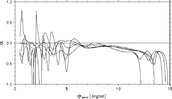
Figure 16: Stability parameter $\alpha$ vs. axial ray angle in the range-averaged AET environment (dashed curve) and in five 650 km block range-averages of the AET environment (solid curves).

Finally, we note that an interesting feature of our ray simulations is that the near-axial rays have much higher stability exponents (typically about $(100\>{\rm km})^{-1}$) than the steeper rays (typically about $(300\>{\rm km})^{-1}$); see Fig. 5. Also, note that Figs. 6 and 7 strongly suggest that the near-axial rays in the AET environment are much more chaotic than the steeper rays. The relative lack of stability of the near-axial rays in the AET environment is, we believe, caused by the background sound speed structure. This topic is discussed in detail in Ref. BVB ; there it is shown that ray stability is largely controlled by a property of the background (which is assumed to be range-independent) sound speed profile, $\alpha=(I/\omega)d\omega/dI$. Large values of $|\alpha|$ are associated with ray instability. $\alpha$ vs axial ray angle in the range-averaged AET environment, and in five 650 km block range-averaged sections of the AET environment, are shown in Fig. 16. (The choice of averaging over 650 km blocks in range is, of course, arbitrary. Range averaging should be done locally, however, because the local sound speed structure may be very different than that which results after averaging over the entire propagation path.) The relatively large near-axial ray values of $|\alpha|$ seen in this figure are consistent with the strongly chaotic nature of these rays seen in Figs. 5, 6 and 7. Unfortunately, the measured wavefield intensity statistics in the AET finale region are not very sensitive to the near-axial ray intensity PDF; as noted above, the argument leading to the expectation that wavefield intensity in the finale region should have an exponential distribution holds for a very large class of ray intensity distributions. Thus, we are not aware of any way that the AET measurements can be used to test our finding that the near-axial rays have larger stability exponents, on average, than the steeper rays.

In summary, we believe that the observed near-lognormal PDF of wavefield intensity for the early resolved AET arrivals is transitional between fluctuations dominated by caustics at short range and saturation at long range, where phase differences will be larger. Surprisingly, for the steep ray AET arrivals phase differences among the steep ray AET arrivals are very small so that saturation has not been reached. The late-arriving AET energy, on the other hand, is characterized by interfering micromultipaths with random phases, leading to an exponential PDF of wavefield intensity. Here, the underlying near-lognormal PDF of ray intensity is obscured. We believe that diffractive effects do not control the intensity fluctuations of either the early or late AET arrivals. Although our theoretical understanding of many of the issues raised in this section is clearly incomplete, it is worth emphasizing that our ray-based numerical simulations of intensity statistics, in which ray trajectories are predominantly chaotic, are in good qualitative agreement with the AET measurements. We do not believe that this agreement is accidental.

V Discussion and summary

In this paper we have seen that in the AET environment, including internal-wave-induced sound speed perturbations, ray trajectories are predominantly chaotic. In spite of extensive ray chaos, many features of ray-based wavefield predictions were shown to be both stable and in good agreement with the AET measurements. Predicted and measured spreads of acoustic energy in time, depth and angle were shown to be in good agreement. It was shown that associated with the chaotic motion of ray trajectories is extensive micromultipathing, and that the micromultipathing process is highly nonlocal; the many micromultipaths that add at the receiver to produce what appears to be a single arrival may sample the ocean very differently. It was shown, surprisingly, that on the early arrival branches the highly nonlocal micromultipathing process causes only very small time spreads and does not lead to a mixing of ray identifiers. A quantitative explanation for the cause of the very small time spreads of the early ray arrivals was presented. Partially heuristic explanations for the near-lognormal and exponential distributions of wavefield intensities for the early and late arrivals, respectively, were provided.

The fact that one is able to make apparently robust and accurate predictions of many wavefield features using ray methods under conditions in which ray trajectories are predominantly chaotic may surprise some readers. Chaotic motion is, after all, intimately linked with unpredictability. This apparent paradox is reconciled by noting that while individual chaotic ray trajectories are unpredictable beyond some short predictability horizon, distributions of chaotic ray trajectories may be quite stable and have robust properties ct . Consider, for example, the motion of the ray whose initial conditions are $z(0)=-652$ m, $\varphi(0)=8.5^{o}$, in the AET environment including a known internal-wave-induced sound speed perturbation. At $r=3252$ km, the depth $z$, angle $\varphi$, travel time $T$, and even the number of turns $M$ made by this ray are likely to be, for all practical purposes, unpredicatble. In contrast, the distribution in $(z,\varphi,T,M)$ of a large ensemble of rays with $z(0)=-652$ m, $8^{o}\leq\varphi(0)\leq 9^{o}$ is very stable in the sense that essentially the same distribution is seen for any large ensemble of randomly chosen (with uniform probability) rays inside this initial angular band. It is the latter property that allows us to make meaningful predictions using an ensemble of chaotic rays in a particular realization of the internal wave field. In addition, ray distributions with similar statistical properties are observed using different realizations of the internal wave field, suggesting that these statistical properties of rays are robust.

Our exploitation of results that relate to ray dynamics, including ray chaos, leads to a blurring of the distinction that is traditionally made between deterministic and stochastic wave propagation problems. The ray dynamics approach emphasizes the distinction between integrable and nonintegrable ray systems, corresponding to range-independent and range-dependent environments, respectively. In generic range-dependent environments at least some ray trajectories will exhibit chaotic motion. The oceanographic origin – mesoscale variability, internal waves or something else – of the range-dependent structure is not critical. An important conceptual insight that can come only from exploitation of results relating to ray chaos is that generically phase space is partitioned into chaotic and nonchaotic regions. This mixture contributes to a combination of limited determinism and constrained stochasticity.

For those who wish to exploit elements of determinism in the propagation physics for the purpose of performing deterministic tomographic inverses, the results that we have presented have important implications. We have seen, for example, that, in spite of extensive ray chaos, many ray-based wavefield descriptors are stable and predictable, and should be invertible. A less encouraging but important observation is that although the travel times of the steep early arrivals are stable and can be inverted, the nonlocality of the micromultipathing process limits one’s ability to invert for range-dependent ocean structure.

For those who wish to understand and predict wavefield statistics, our results also have important implications. These comments are based on our analysis of the AET measurements, but are expected to apply to a large class of long-range propagation problems. First, we have seen that stable and unstable ray trajectories coexist and that this influences wavefield intensity statistics. Second, we have seen that micromultipathing is extensive and highly nonlocal. The strongly nonlocal nature of the micromultipathing process is significant because: a) this process cannot be modelled using a perturbation analysis which assumes the existance of an isolated background ray path; and b) the effects of this process will not, in general, be eliminated as a result of local smoothing by finite frequency effects. Third, we have seen that the appearance of stochastic effects is not entirely due to internal waves. We have seen, for example, that, even in the absence of internal waves, near-axial rays in the AET environment are chaotic. Recall that we noted in the introduction that part of the motivation for the present study was to understand the reasons underlying the finding of Colosi et al. AET2 that the theory described in Ref. FDMWZ fails to correctly predict the AET wavefield statistics. This failure is not surprising in view of the observation that this theory is based on assumptions that either explicitly violate, or lead to the violation of, all three of the aforementioned properties of the scattered wavefield. Note also in this regard that the combination of extensive micromultipathing, small time spreads, and lognormally distributed intensities that characterizes the early AET arrivals is not consistent with any of the three propagation regimes identified in this theory.

Although we have argued that a ray-based wavefield description which relies heavily on results relating to ray chaos can account for all of the important features of the AET measurements, it should be emphasized that our analysis has some shortcomings. Recall that our simulations using $E=0.5\>E_{GM}$ resulted in steep arrival time spreads and peak intensity statistics in good agreement with measurements, but that simulations using $E=1.0\>E_{GM}$ did not, although direct measurements favor $E=1.0\>E_{GM}$. We have not provided a rigorous argument to establish the connection between a near-lognormal ray intensity PDF and a near-lognormal wavefield intensity PDF. Indeed, a complete theory of wavefield statistics which accounts for complexities associated with ray chaos is lacking. This is closely linked to the subject of wave chaos rdoa , which is currently not well understood. Also, we have only briefly discussed the spreads of energy in depth and angle, and more work needs to be done on quantifying time spreads.

Finally, we wish to remark that the importance of ray methods is not diminished by recent advances, both theoretical and computational, in the development of full wave models, such as those based on parabolic equations. The latter are indispensible computational tools in many applications. In contrast, the principal virtue of ray methods is that they provide insight into the underlying wave propagation physics that is difficult, if not impossible, to obtain by any other means. The results presented in this paper illustrate this statement.

Acknowledgments

We thank Fred Tappert and Frank Henyey for the benefit of discussions on many of the topics included in this paper, and the ATOC group (A. B. Baggeroer, T. G. Birdsall, C. Clark, B. D. Cornuelle, D. Costa, B. D. Dushaw, M. A. Dzieciuch, A. M. G. Forbes, B. M. Howe, D. Menemenlis, J. A. Mercer, K. Metzger, W. Munk, R. C. Spindel, P. F. Worcester and C. Wunsch) for giving us access to the AET acoustic and environmental measurements. This work was supported by Code 321 OA of the U.S. Office of Naval Research.

References

- (1) S. S. Abdullaev and G. M. Zaslavsky, “Stochastic instability of rays and the spekle structure of the field in inhomogeneous media,” Zh. Eksp. Teor. Fiz. 87, 763-775 (1984) [Engl. transl.: Sov. Phys. JETP 60, 435-441 (1985)].
- (2) D. R. Palmer, M. G. Brown, F. D. Tappert and H. F. Bezdek, “Classical chaos in nonseparable wave propagation problems,” Geophys. Res. Lett. 15, 569-572 (1988).
- (3) S. S. Abdullaev and G. M. Zaslavsky, “Fractals and ray dynamics in longitudinally inhomogeneous media,” Sov. Phys. Acoust. 34, 334-336 (1989).
- (4) S. S. Abdullaev and G. M. Zaslavskii, “Classical nonlinear dynamics and chaos of rays in wave propagation problems in inhomogeneous media,” Usp. Phys. Nauk 161, 1-43 (1991).
- (5) M. G. Brown, F. D. Tappert and G. Goñi, “An investigation of sound ray dynamics in the ocean volume using an area-preserving mapping,” Wave Motion 14, 93-99 (1991).
- (6) F. D. Tappert, M. G. Brown and G. Goñi, “Weak chaos in an area-preserving mapping for sound ray propagation,” Phys. Lett. A 153, 181-185 (1991).
- (7) M. G. Brown, F. D. Tappert, G. Goñi and K. B. Smith, “Chaos in underwater acoustics,” in Ocean Variability and Acoustic Propagation, edited by J. Potter and A. Warn-Varnas (Kluwer Academic, Dordrect, 1991), 139-160.
- (8) D. R. Palmer, T. M. Georges and R. M. Jones, “Classical chaos and the sensitivity of the acoustic field to small-scale ocean structure,” Comput. Phys. Commun. 65, 219-223 (1991).
- (9) K. B. Smith, M. G. Brown and F. D. Tappert, “Ray chaos in underwater acoustics,” J. Acoust. Soc. Am. 91, 1939-1949 (1992).
- (10) K. B. Smith, M. G. Brown and F. D. Tappert, “Acoustic ray chaos induced by mesocsale ocean structure,” J. Acoust. Soc. Am. 91, 1950-1959 (1992).
- (11) S. S. Abdullaev, Chaos and Dynamics of Rays in Waveguide Media, Edited by G. Zaslavsky (Gordon and Breach science publishers, 1993).
- (12) F. D. Tappert and X. Tang, “Ray chaos and eigenrays,” J. Acoust. Soc. Am. 99, 185-195 (1996).
- (13) G. M. Zaslavsky and S. S. Abdullaev, “Chaotic transmission of waves and ‘cooling’ of signals,” Chaos 7, 182-186 (1997).
- (14) J. Simmen, S. M. Flatté and G.-Yu Wang, “Wavefront folding, chaos and diffraction for sound propagation through ocean internal waves,” J. Acoust. Soc. Am. 102, 239-255 (1997).
- (15) M. G. Brown, “Phase space structure and fractal trajectories in 1 1/2 degree of freedom Hamiltonian systems whose time dependence is quasiperiodic,” Nonlinear Processes in Geophys. 5, 69-74 (1998).
- (16) M. Wiercigroch, M. Badiey, J. Simmen and A. H.-D. Cheng. “Nonlinear dynamics of underwater acoustics,” J. Sound Vibr. 220, 771-786 (1999).
- (17) B. Sundaram and G. M. Zaslavsky, “Wave analysis of ray chaos in underwater acoustics,” Chaos 9, 483-492 (1999).
- (18) M. A. Wolfson and F. D. Tappert, “Study of horizontal multipaths and ray chaos due to ocean mesoscale structure,” J. Acoust. Soc. Am. 107, 154-162 (2000).
- (19) A. L. Virovlyansky and G. M. Zaslavsky, “Evaluation of the smoothed interference pattern under conditions of ray chaos,” Chaos 10, 211-223 (2000).
- (20) M. A. Wolfson and S. Tomsovic, “On the stability of long-range sound propagation through a structured ocean,” J. Acoust. Soc. Am. 109, 2693-2703 (2001); nlin.CD/0002030.
- (21) I. P. Smirnov, A. L. Virovlyansky and G. M. Zaslavsky, “ Theory and application of ray chaos to the underwater acoustics,” Phys. Rev. E 64 366221 (2001).
- (22) M. G. Brown, J. A. Colosi, S. Tomsovic, A. L. Virovlyansky, M. A. Wolfson and G. M. Zaslavsky, “Ray dynamics in ocean acoustics,” submitted to J. Acoust. Soc. Am. (2001); nlin.CD/0109027.
- (23) P. F. Worcester, B. D. Cornuelle, M. A. Dzieciuch, W. H. Munk, B. M. Howe, J. A. Mercer, R. C. Spindel, J. A. Colosi, K. Metzger, T. Birdsall and A. B. Baggeroer, “A test of basin-scale acoustic thermometry using a large- aperture vertical array at 3250-km range in the eastern North Pacific Ocean,” J. Acoust. Soc. Am. 105, 3185-3201 (1999).
- (24) J. A. Colosi, E. K. Scheer, S. M. Flatté, B. D. Cornuelle, M. A. Dzieciuch, W. H. Munk, P. F. Worcester, B. M. Howe, J. A. Mercer, R. C. Spindel, K. Metzger, T. Birdsall and A. B. Baggeroer, “Comparisons of measured and predicted acoustic fluctuations for a 3250-km propagation experiment in the eastern North Pacific Ocean,” J. Acoust. Soc. Am. 105, 3202-3218 (1999).
- (25) J. A. Colosi, F. Tappert and M. Dzieciuch, “Further analysis of intensity fluctuations from a 3252-km acoustic propagation experiment in the eastern North Pacific Ocean,” J. Acoust. Soc. Am. 110, 163-169 (2000).
- (26) J. L. Spiesberger, R. C. Spindel and K. Metzger, “Stability and identification of ocean acoustic multipaths,” J. Acoust. Soc. Am. 67, 2011-2917 (1980).
- (27) P. F. Worcester, B. D. Cornuelle, J. A. Hildebrand, W. S. Hodgkiss, Jr., T. F. Duda, J. Boyd, B. M. Howe, J. A. Mercer and R. C. Spindel, “A comparison of measured and predicted broadband acoustic arrival patterns in travel time-depth coordinates at 1000 km range,” J. Acoust. Soc. Am. 95, 3118-3128 (1994).
- (28) T. F. Duda, S. M. Flatté, J. A. Colosi, B. D. Cornuelle, J. A. Hildebrand, W. S. Hodgkiss, Jr., P. F. Worcester, B. M. Howe, J. A. Mercer and R. C. Spindel, “Measured wavefront fluctuations in 1000-km pulse propagation in the Pacific Ocean,” J. Acoust. Soc. Am. 92, 939-955 (1992).
- (29) J. A. Colosi, S. M. Flatté and C. Bracher, “Internal-wave effects on 1000-km oceanic acoustic pulse propagation: Simulation and comparison with experiment,” J. Acoust. Soc. Am. 96, 452-468 (1994).
- (30) M. A. Wolfson and J. L. Spiesberger, “Full wave simulation of the forward scattering of sound in a structured ocean: A comparison with observations,” J. Acoust. Soc. Am. 106, 1293-1306 (1999).
- (31) S. Flatté, R. Dashen, W. Munk, K. Watson and F. Zachariasen, Sound Transmission through a Fluctuating Ocean (Cambridge University Press, Cambridge, 1979).
- (32) J. A. Colosi and S. M. Flatté, “Mode coupling by internal waves for multimegameter acoustic propagation in the ocean,” J. Acoust. Soc. Am. 100, 3607-3620 (1996).
- (33) W. H. Munk, “Internal waves and small scale processes,” in Evolution of Physical Oceanography, edited by B. A. Warren and C. Wunsch (MIT Press, Cambridge, 1981), 264-291.
- (34) J. A. Colosi and M. G. Brown, “Efficient numerical simulation of stochastic internal-wave-induced sound speed perturbation fields,” J. Acoust. Soc. Am. 103, 2232-2235 (1998).
- (35) W. H. Munk, “Sound channel in an exponentially stratified ocean with application to SOFAR,” J. Acoust. Soc. Am. 55, 220-226 (1974).
- (36) A. L. Virovlyansky, “Ray travel times at long range in acoustic waveguides,” submitted to J. Acoust. Soc. Am. (2001).
- (37) A. L. Virovlyansky, “Ray travel times in range-dependent acoustic waveguides,” submitted to J. Acoust. Soc. Am. (2001); nlin.CD/0012015.
- (38) J. A. Colosi, “A review of recent results on ocean acoustic wave propagation in random media: basin scales,” IEEE J. of Oceanic Engineering 24, 138-155 (1999).
- (39) M. V. Berry, “Focusing and twinkling: critical exponents from catastophes in non-Gaussian random short waves,” J. Phys. A. Math. Gen. 10, 2061-2081 (1977).
- (40) J. G. Walker, M. V. Berry and C. Upstill, “Measurements of twinkling exponents of light focused by randomly rippling water,” Optica Acta 30, 1001-1010 (1983).
- (41) J. H. Hannay, “Inensity fluctuations beyond a one-dimensional random refracting screen in the short-wavelength limit,” Optica Acta 29, 1631-1649 (1982).
- (42) G. M. Zaslavsky, Physics of Chaos in Hamiltonian Systems (Imperial College Press, London, 1998).
- (43) M. Tabor, Chaos and Integrability in Nonlinear Dynamics (Wiley-Interscience, New York, 1989).
- (44) F. J. Beron-Vera and M. G. Brown, “Ray stability in weakly range-dependent sound channels,” to be submitted to J. Acoust. Soc. Am. (2002).
- (45) N. R. Cerruti and S. Tomsovic, “Sensitivity of wave field evolution and manifold stability in perturbed chaotic systems,” Phys. Rev. Lett. 88, 054103 (2002); nlin.CD/0108016.