Resonant triad dynamics in weakly damped Faraday waves with two-frequency forcing

Abstract

Many of the interesting patterns seen in recent multi-frequency Faraday experiments can be understood on the basis of three-wave interactions (resonant triads). In this paper we consider two-frequency forcing and focus on a resonant triad that occurs near the bicritical point where two pattern-forming modes with distinct wavenumbers emerge simultaneously. This triad has been observed directly (in the form of rhomboids) and has also been implicated in the formation of quasipatterns and superlattices. We show how the symmetries of the undamped unforced problem (time translation, time reversal, and Hamiltonian structure) can be used, when the damping is weak, to obtain general scaling laws and additional qualitative properties of the normal form coefficients governing the pattern selection process near onset; such features help to explain why this particular triad is seen only for certain “low” forcing ratios, and predict the existence of drifting solutions and heteroclinic cycles. We confirm the anticipated parameter dependence of the coefficients and investigate its dynamical consequences using coefficients derived numerically from a quasipotential formulation of the Faraday problem due to Zhang and Viñals.

,

1 Introduction

When a container of fluid is shaken vertically with sufficient strength, patterns of standing waves (SW) develop on the free surface. This well-known transition, first described by Faraday [1], is one of the best known examples of a pattern forming instability. At a critical value of the forcing amplitude the flat surface loses stability and, with the aid of small perturbations, gives way to a spatially structured state. This excited state is often highly ordered and has been observed in the form of rolls, squares, hexagons, and more exotic structures such as superlattices and quasi-patterns having 8, 10, or 12-fold rotational symmetry [2, 3, 4, 5, 6]. The temporal spectrum of these resonant SW oscillations is highly ordered as well. In the standard Faraday experiment with single frequency forcing of period $T=2\pi/\omega$ the first pattern to appear is a subharmonic response, i.e., it is $2T$-periodic in time [7]. The characteristic wavenumber $k$ of the pattern is determined by the dispersion relation $\Omega(k)$ for gravity-capillary waves through the subharmonic resonance condition $\Omega(k)=\omega/2$. This frequency $\omega$, which controls the spatial length scale, and the forcing amplitude $f$ are the most readily accessible control parameters.

Recently, a number of investigators [4, 5, 6, 8, 9, 10, 11, 12] have looked at more general kinds of periodic forcing. Such forcing functions have multiple frequency components and present a larger number of adjustable parameters. One of the biggest advantages to using multiple frequencies is that one can study, in a controlled manner, the competition between modes of different length scales. If the applied acceleration $f(t)$ is composed of two commensurate frequencies of ratio $m$:$n$ ($m$ and $n$ coprime):

$$f(t) =\frac{1}{2}\left(f_{m}e^{im\omega t}+f_{n}e^{in\omega t}+c.c.\right)=|f_{m}|\cos(m\omega t+\phi_{m})+|f_{n}|\cos(n\omega t+\phi_{n}),$$ (1)

an appropriate balance between $|f_{m}|$ and $|f_{n}|$ ensures that the two modes (one driven primarily by the $f_{m}$ forcing component and the other by $f_{n}$) onset simultaneously. This bicritical point is the natural organizing center for the two-frequency problem because it is at this point that the greatest variety of patterns evolve and compete with each other while still in the weakly nonlinear regime. A complete description of this competition is exceedingly difficult to achieve, yet a number of simple resonant interactions have emerged as crucial building blocks for many of the more interesting patterns. In this respect resonant triads are particularly influential because they are the lowest order nonlinear effect (i.e., they arise at second order in a weakly nonlinear expansion) and provide a strong phase coupling between the three waves involved. They have been implicated in a number of pattern formation studies, both experimental [3, 4, 5, 8, 13] and theoretical [10, 14, 15, 16, 17].

In this paper we consider the two-frequency forcing of Eq. (1) and focus on a simple three-wave interaction, occurring near the bicritical point, in which two wavevectors from one critical circle, ${\boldsymbol{k}}_{1}$ and ${\boldsymbol{k}}_{2}$, sum to give a third wavevector ${\boldsymbol{k}}_{3}$ on the second critical circle (see Fig. 1).

Figure 1: Resonant triad interactions at the bicritical point: (a) when $k_{3}<k_{1}$ and (b) when $k_{1}<k_{3}<2k_{1}$.

Patterns formed by these three SW modes were called two-mode rhomboids by Arbell and Fineberg [8]. The same basic resonance, however, was shown to be an essential component of more complicated states such as quasipatterns with 8-fold or 10-fold symmetry [8] (the former observed with three-frequency forcing [3]), and several other multiple mode and modulated states [3]. One of the most striking facts about this resonant triad is that it has so far been seen only with forcing ratios of 1:2 (as part of a superlattice-II type state [3]), 2:3, and 4:5. In [9] we showed that the absence of two-mode rhomboids for larger values of $m$ and $n$ is related to the presence of (broken) time translation symmetry. This paper provides additional details behind that result as well as others in [9], and explores their dynamical implications.

Symmetry arguments, in general, play a central role in our understanding of pattern formation, providing a powerful framework that explains generic features, i.e., properties that one expects to find across a wide range of physical systems sharing the same symmetry. For Faraday systems of large aspect ratio (i.e., where the horizontal extent of the system is large compared to the characteristic wavelength) the relevant symmetry is that of the plane, described by the Euclidean group E(2). If the pattern is spatially periodic, as is often the case near onset, many useful results (see, e.g., [18, 19]) can be obtained by restricting to patterns commensurate with this periodic lattice. The choice of a lattice fixes the orientation and removes the arbitrary rotations that are part of E(2). Spatial translations, however, are still allowed, as are certain discrete rotations ($60^{\circ}$ for hexagons, for example) and reflections. Thus, when periodic planforms are considered the noncompact group E(2) is replaced by a compact group, namely, the semi-direct product of a discrete group representing the lattice symmetries (this group is $D_{2}$ for the resonant triads we consider) and the two-torus representing spatial translations. The fact that these symmetry operations must transform a given solution into an equivalent solution restricts the form of the equations governing the pattern formation process near onset and thus determines which types of nonlinear terms can be present and which cannot [18].

Temporal symmetries also play an important role in periodically forced systems. In particular, such systems are invariant under discrete translation through one forcing period: $t\rightarrow t+T$. Whether this symmetry is important or not depends on the nature of the linear eigenfunctions. In the case of single-frequency forcing, for example, the eigenfunctions are subharmonic (i.e., they have odd parity under $t\rightarrow t+T$) and the associated ${\mathbb{Z}}_{2}$ symmetry bars all even terms from the evolution equations; in particular, the absence of quadratic terms means that there are no resonant triad interactions. With two-frequency forcing the restrictions due to discrete temporal translation are less severe because the period $T$ is longer than the corresponding period for, say, isolated $m\omega$ forcing, which would be $T/m$. In this way, modes driven “subharmonically” by $f_{m}$ may actually be harmonic with respect to the full period $T$; they are harmonic if $m$ is even and subharmonic if $m$ is odd, similarly for $n$.

In this paper we follow the approach outlined in [9] and extend the usual analysis based on “exact” spatial symmetries and discrete time translation to include the approximate (i.e., weakly broken) symmetries of continuous time translation, time reversal, and Hamiltonian structure. In [9] we considered hexagons and two-mode superlattices [3, 5] as well as two-mode rhomboids, and showed how these symmetries can be used to determine the leading order dependence of important coefficients in the SW amplitude equations. In this paper we supply the details of that calculation for the case of two-mode rhomboids (here simply referred to as resonant triads) and explore the dynamical consequences of its predictions. For example, in Section 4 we show that a preference for resonant coefficients of opposite sign [9], which stems from the presence of Hamiltonian structure in the undamped problem, leads to the existence of drifting solutions, modulated waves, and heteroclinic cycles.

The organization of the paper is as follows. In Section 2 we demonstrate how the broken temporal symmetries can be replaced by unbroken parameter symmetries (see also [9]), and use these in conjunction with the spatial symmetries to determine not only the form of the SW amplitude equations but also the manner in which the coefficients of these equations depend on the forcing parameters ($m$, $n$, $|f_{m}|$, $|f_{n}|$, $\phi_{m}$, $\phi_{n}$) and on the damping. In Section 3 we test our symmetry-based predictions against coefficients calculated numerically from a quasipotential formulation of the Faraday problem due to Zhang and Viñals [14, 15]. Section 4 summarizes the typical dynamics associated with the resonant triad equations and uses numerical examples to illustrate the effects of the broken symmetries discussed in Section 2. In Section 5 we offer our conclusions.

2 Derivation of the Amplitude Equations

In this section we use general symmetry arguments to derive the form of the equations governing resonant triads in the presence of two-frequency forcing (Eq. (1)). In particular, we obtain general scaling properties of the normal form coefficients. These scaling laws rest on the assumption of weak dissipation (the critical forcing amplitude needed to destabilize the spatially uniform state is then similarly small). In this limit the problem is constrained not only by spatial symmetries but by the (weakly broken) symmetries of time translation $t\rightarrow t+s$, $s\in{\mathbb{R}}$ and time reversal $t\rightarrow-t$ that are features of the unforced inviscid hydrodynamical problem. In fact, if these two symmetries are extended in an appropriate way (see Section 2.2) they apply to the damped forced problem as well. Additional constraints resulting from full Hamiltonian structure in the undamped forced problem are examined in Section 2.3.1.

There are many adjustable parameters in the two-frequency Faraday experiment. In addition to the fluid depth (assumed to be infinite in our numerical study; see Section 3) and properties such as viscosity $\nu$, density $\rho$, and surface tension $\Gamma$, one can vary the basic frequency $\omega$ of the driving, the ratio of the two frequency components $m$:$n$, their respective magnitudes $|f_{m}|$ and $|f_{n}|$, and their phases $\phi_{m}$ and $\phi_{n}$. Here we take $1/\omega$ as the unit of time, writing $\tau=\omega t$, and use the wavenumber $k_{0}$ associated with $\Omega_{0}\equiv{\rm min}(m,n)\omega/2$ via the inviscid dispersion relation $g_{0}k_{0}+\Gamma k_{0}^{3}/\rho=\Omega_{0}^{2}$ ($g_{0}$ is the acceleration of gravity) as the inverse unit of length. This scaling groups $\omega$, $\nu$, $\Gamma$, and $\rho$ into three nondimensional parameters: $\gamma\equiv 2\nu k_{0}^{2}/\omega$ (the damping), $\Gamma_{0}\equiv\Gamma k_{0}^{3}/(\rho\omega^{2})$ (the capillarity number), and $G_{0}\equiv g_{0}k_{0}/\omega^{2}$ (the gravity number). The last two are related by the equation $\Gamma_{0}+G_{0}=({\rm min}(m,n)/2)^{2}$.

The situation of special interest here is the bicritical point where two modes of distinct wavenumber are simultaneously excited as the overall forcing amplitude $f\equiv(|f_{m}|^{2}+|f_{n}|^{2})^{1/2}$ is increased (see Fig. 2).

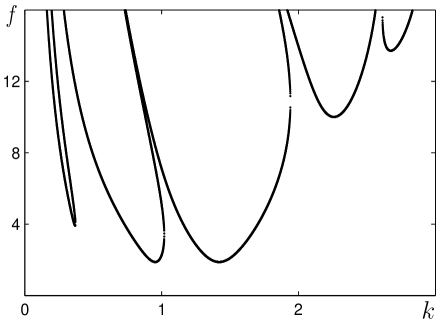
Figure 2: Neutral stability curves at the bicritical point calculated from the Zhang-Viñals equations (see Section 3). We use $m$:$n=3$:2, $\gamma=0.1$, $\Gamma_{0}=0.5$, $G_{0}=0.5$, $\phi_{m}=\phi_{n}=0$ and $|f_{2}|/|f_{3}|\simeq 0.423$. The applied acceleration $f$ is in units of $g_{0}$.

We think of this bistability criteria as determining the ratio $|f_{m}|/|f_{n}|$.

The two critical circles at the bicritical point and the two different ways of constructing a resonant triad are illustrated in Fig. 1. In either case we choose three wavevectors: two of equal magnitude, $|{\boldsymbol{k}}_{1}|=|{\boldsymbol{k}}_{2}|=k_{1}$, and their sum, ${\boldsymbol{k}}_{3}={\boldsymbol{k}}_{1}+{\boldsymbol{k}}_{2}$. Without loss of generality we associate ${\boldsymbol{k}}_{1}$ and ${\boldsymbol{k}}_{2}$ with the $f_{m}$ forcing component and ${\boldsymbol{k}}_{3}$ with the $f_{n}$ component. Thus Fig. 1a applies if $m>n$ while Fig. 1b applies if $m<n$. As mentioned, when the damping is small each of the excited modes can, to first approximation, be thought of as a subharmonic response to the corresponding component ($f_{m}$ or $f_{n}$) of the driving. The $\exp\{i{\boldsymbol{k}}_{1}\cdot{\boldsymbol{x}}\}$ and $\exp\{i{\boldsymbol{k}}_{2}\cdot{\boldsymbol{x}}\}$ modes oscillate with a dominant frequency of $m/2$ while the $\exp\{i{\boldsymbol{k}}_{3}\cdot{\boldsymbol{x}}\}$ mode has dominant frequency $n/2$. A given mode is harmonic (subharmonic) when $m$ or $n$ is even (odd). As shown in Section 2.2, resonant triads only occur if $n$ is even, in which case $m$ is odd since $m$ and $n$ are coprime.

As long as damping is present the first modes to appear as $f$ is increased are SW. Sufficiently close to onset the resonant triad system may therefore be described by the three complex amplitudes $A_{j}$, $j=1,2,3$ of the SW modes $\exp\{i\boldsymbol{k}_{j}\cdot\boldsymbol{x}\}$. We do not begin immediately with these three SW modes but, following the program of [9], obtain first the form of the equations governing six traveling wave (TW) modes having the same wavevectors ${\boldsymbol{k}}_{1}$, ${\boldsymbol{k}}_{2}$, and ${\boldsymbol{k}}_{3}$. It should be noted that in the absence of dissipation and forcing the Faraday system supports TW at infinitely many frequencies and wavenumbers, i.e., the only requirement is from the inviscid dispersion relation $\Omega(k)$. It is precisely the applied forcing which selects, through the temporal resonance condition, the frequencies and hence the length scales of the problem. Our approach, by restricting attention to the wavenumbers $k_{1}$ and $k_{3}$, anticipates the effect of the parametric forcing. At the same time, however, it assumes that the amplitude of this forcing (and of the damping) is small. In this limit a TW expansion is justified despite the fact that pure TW solutions are destroyed by the parametric forcing term – such an approach may also be viewed as the unfolding of a Hopf bifurcation (occurring at $\gamma=0$) with nearly resonant temporal forcing (see [20, 21]). Here we are motivated in our use of TW by the action of the weakly broken temporal symmetries; TW transform in a simple way under time translation $\tau\rightarrow\tau+s$ and time reversal $\tau\rightarrow-\tau$ whereas SW do not. The simple transformation properties of TW allow us to take full advantage of the spatial and temporal symmetries before a center manifold reduction is used to obtain the equations describing the three SW amplitudes $A_{j}$.

We now systematically consider the two unfolding parameters which move the system away from the “ideal” undamped, unforced case: the damping parameter $\gamma>0$ (proportional to viscosity) that breaks time reversal symmetry, and the forcing function $f(\tau)$ (equivalently, $f_{m}$ and $f_{n}$), which breaks the continuous time translation symmetry and, in general, the time reversal symmetry as well. In the process we pay special attention to resonant terms, i.e., those terms which couple the phases of the different modes, because of the crucial role they play in the ensuing dynamics. The leading resonant terms are quadratic in amplitude but, with the exception of $m$:$n$ = 1:2, appear only as a result of broken time translation symmetry. The residual effect of this symmetry determines, for small $\gamma$, the influence (i.e., size) of these resonant terms by prescribing how they scale with the symmetry-breaking parameters $f_{m}$ and $f_{n}$.

2.1 Traveling wave equations

We consider a system of six undamped, unforced TW with wavevectors ${\boldsymbol{k}}_{1}$, ${\boldsymbol{k}}_{2}$, and ${\boldsymbol{k}}_{3}$. For example, the surface height $h({\boldsymbol{x}},\tau)$ is written as

$$h({\boldsymbol{x}},\tau)= \,Z_{1}^{+}e^{i({\boldsymbol{k}}_{1}\cdot{\boldsymbol{x}}+m\tau/2)}+Z_{1}^{-}e^{i({\boldsymbol{k}}_{1}\cdot{\boldsymbol{x}}-m\tau/2)}+Z_{2}^{+}e^{i({\boldsymbol{k}}_{2}\cdot{\boldsymbol{x}}+m\tau/2)}+Z_{2}^{-}e^{i({\boldsymbol{k}}_{2}\cdot{\boldsymbol{x}}-m\tau/2)}$$

$$\,Z_{3}^{+}e^{i({\boldsymbol{k}}_{3}\cdot{\boldsymbol{x}}+n\tau/2)}+Z_{3}^{-}e^{i({\boldsymbol{k}}_{3}\cdot{\boldsymbol{x}}-n\tau/2)}+c.c.+...\,.$$ (2)

The equations describing the slow evolution of the TW amplitudes $Z_{j}^{\pm}$, $j=1,2,3$ must be equivariant under the operations of spatial translation (${\cal T}_{\boldsymbol{\phi}}$), reflection ($\kappa$) about a line through ${\boldsymbol{k}}_{3}$, and rotation ($\cal R$) by $\pi$ (i.e., inversion through the origin):

$${\cal T}_{\boldsymbol{\phi}} :Z_{j}^{\pm}\rightarrow Z_{j}^{\pm}e^{i\phi_{j}},\quad{\boldsymbol{\phi}}=(\phi_{1},\phi_{2}),\quad\phi_{1},\phi_{2}\in[0,2\pi),\quad\phi_{3}=\phi_{1}+\phi_{2},$$ (3)

$$\kappa :Z_{1}^{\pm}\leftrightarrow Z_{2}^{\pm},$$ (4)

$${\cal R} :Z_{j}^{\pm}\rightarrow\bar{Z}_{j}^{\mp}.$$ (5)

In the absence of forcing ($f$) the equations must also be equivariant under time translation:

$${\cal T}_{s}:(Z_{1}^{\pm},Z_{2}^{\pm}) \rightarrow(Z_{1}^{\pm},Z_{2}^{\pm})e^{\pm ims/2},\qquad Z_{3}^{\pm} \rightarrow Z_{3}^{\pm}e^{\pm ins/2},\qquad s\in[0,4\pi),$$ (6)

while if both $f$ and $\gamma$ are zero there is the time reversal symmetry $\sigma$:

$$\sigma\,:\,\tau\rightarrow-\tau,\quad Z_{j}^{\pm}\rightarrow Z_{j}^{\mp},$$ (7)

The constraints of symmetries (3-7) lead to equations, truncated at cubic order, of the form

$$\dot{Z}_{1}^{+}=\, \{\tilde{\alpha}\bar{Z}_{2}^{+}Z_{3}^{+}\}_{1:2}+\delta Z_{2}^{+}\bar{Z}_{2}^{-}Z_{1}^{-}$$

$$+ \left({\rm a}|Z_{1}^{+}|^{2}+{\rm b}|Z_{1}^{-}|^{2}+{\rm c}|Z_{2}^{+}|^{2}+{\rm d}|Z_{2}^{-}|^{2}+{\rm e}|Z_{3}^{+}|^{2}+{\rm f}|Z_{3}^{-}|^{2}\right)Z_{1}^{+},$$ (8)

$$\dot{Z}_{3}^{+}=\, \{\tilde{\beta}Z_{1}^{+}Z_{2}^{+}\}_{1:2}+\left({\rm g}(|Z_{1}^{+}|^{2}+|Z_{2}^{+}|^{2})+{\rm h}(|Z_{1}^{-}|^{2}+|Z_{2}^{-}|^{2})+{\rm l}|Z_{3}^{+}|^{2}+{\rm p}|Z_{3}^{-}|^{2}\right)Z_{3}^{+},$$ (9)

where the overdot indicates a derivative with respect to $\tau$. The other four equations follow from the symmetries $\kappa$ and ${\cal R}$. The quadratic terms in curly brackets (subscript 1:2) are permitted only when $m$:$n$ = 1:2 because with other forcing ratios they violate the time translation symmetry ${\cal T}_{s}$. Whether these resonant terms are present or not, the time reversal symmetry $\sigma$ (more precisely, $\sigma\circ{\cal R}$) forces all coefficients to be purely imaginary:

$$\tilde{\alpha}=i\tilde{\alpha}_{i},\quad\delta=i\delta_{i},\quad a=ia_{i},\quad...,\quad p=ip_{i}.$$ (10)

The absence of linear terms with imaginary coefficients is not related to symmetry but to the way we define $k_{1}$ and $k_{3}$, which requires that the detuning vanish at $f=\gamma=0$. To see this, recall that expansion (2) anticipates finite damping and forcing in two ways: it assumes the TW modes are in subharmonic resonance with the two driving frequencies, i.e., they oscillate at $m/2$ or $n/2$, and it takes the wavenumbers $k_{1}$ and $k_{3}$ from the $\gamma$-dependent dual minima of the SW neutral stability curves at the bicritical point of the damped forced problem not from the dispersion relation, $\Omega(k_{1})=m/2$ and $\Omega(k_{3})=n/2$. One consequence of this implicit $\gamma$ dependence in $k_{1}$ and $k_{3}$ is a detuning in the damped forced problem between the parametrically excited frequencies $m/2$ and $n/2$ and the “natural” frequencies $\Omega(k_{1})$ and $\Omega(k_{3})$. In Eqs. (8,9) however, the damping and forcing are both zero, and the wavenumbers $k_{1}$ and $k_{3}$ coincide with those given by the inviscid dispersion relation, i.e., $\Omega(k_{1})=m/2$ and $\Omega(k_{3})=n/2$. Consequently, there is no detuning at $f=\gamma=0$.

2.2 Unfolding of Eqs. (8-9): parameter symmetries

We now unfold the vector field (8,9) assuming all symmetry-breaking parameters are the same order: $|f_{m}|\sim|f_{n}|\sim\gamma\sim\epsilon$. Throughout this unfolding we will be interested only in those terms which add new qualitative effects or determine the leading order scaling of coefficients in the subsequent SW equations. Assuming that the symmetry-breaking terms are analytic in $f$ and $\gamma$, their precise form can be obtained by appealing to a more general class of symmetries in which parameters may be transformed along with dynamical variables (see, e.g., [22]). In this way the broken symmetries ${\cal T}_{s}$ and $\sigma$ can be recast in terms of intact parameter symmetries. Put another way, it is still possible to translate or reflect the problem in time so long as the damping and forcing terms are also appropriately transformed. Specifically, we have the parameter symmetry

$${\cal T}_{s}^{\rm par}:\, (Z_{1}^{\pm},Z_{2}^{\pm})\rightarrow(Z_{1}^{\pm},Z_{2}^{\pm})e^{\pm ims/2},\qquad Z_{3}^{\pm}\rightarrow Z_{3}^{\pm}e^{\pm ins/2},$$

$$(f_{m},f_{n})\rightarrow(f_{m}e^{ims},f_{n}e^{ins}),$$ (11)

replacing ${\cal T}_{s}$, while $\sigma$ becomes

$$\sigma^{\rm par}\,:\,(\tau,\gamma)\rightarrow-(\tau,\gamma),\quad Z_{j}^{\pm}\rightarrow Z_{j}^{\mp},\quad(f_{m},f_{n})\rightarrow(\bar{f}_{m},\bar{f}_{n}).$$ (12)

Although parameter symmetries are sometimes unphysical (it makes little sense to take $\gamma<0$) they are perfectly good mathematical symmetries of the governing equations and may be used to advantage - in this case they yield the proper form of symmetry-breaking terms.

2.2.1 Finite forcing: $f\neq 0$

The presence of forcing allows several new terms in Eqs. (8,9). For example, at linear order in amplitude Eq. (8) contains the usual parametric forcing term $f_{m}Z_{1}^{-}$, consistent with the symmetry ${\cal T}_{s}^{\rm par}$. Another important addition comes in the form of quadratic resonance terms. The quadratic amplitude dependence follows from the spatial resonance condition (3) but the dependence on $f_{m}$ and $f_{n}$ can only be determined with the help of ${\cal T}_{s}^{\rm par}$, i.e., it reflects a temporal resonance requirement. To determine this dependence we consider adding terms, consistent with the spatial resonance requirement, of the form $f_{m}^{r}f_{n}^{u}\bar{Z}_{2}^{\pm}Z_{3}^{\pm}$ and $f_{m}^{v}f_{n}^{w}Z_{1}^{\pm}Z_{2}^{\pm}$ to Eqs. (8) and (9), respectively. Here $r$ ,$u$, $v$, and $w$ are integers, allowed to be negative to indicate complex conjugation (i.e., $f_{m}^{-2}\equiv\bar{f}_{m}^{2}$ and so on). A combination such as $f_{m}\bar{f}_{m}$ is invariant under ${\cal T}_{s}^{\rm par}$ and appears only at higher order. The temporal resonance condition, which follows from the equivariance requirement under ${\cal T}_{s}^{\rm par}$, may be expressed as

$$m/2 =r\,m+u\,n-\varepsilon_{1}m/2+\varepsilon_{2}n/2,$$ (13)

$$n/2 =v\,m+w\,n+\varepsilon_{3}m/2+\varepsilon_{4}m/2,$$ (14)

where $\varepsilon_{i}=\pm 1$, $i=1,...,4$. These $\varepsilon_{i}$ distinguish between the $Z_{j}^{+}$ modes (the corresponding $\varepsilon_{i}$ are positive) and the $Z_{j}^{-}$ modes (negative $\varepsilon_{i}$). We seek values for the parameters $r$, $u$, $v$, $w$, $\varepsilon_{1}$, $\varepsilon_{2}$, $\varepsilon_{3}$, and $\varepsilon_{4}$ that minimize both $|r|+|u|$ and $|v|+|w|$ and therefore give resonance terms of lowest order in $f$. To accomplish this we rewrite Eqs. (13) and (14):

$$m(1+\varepsilon_{1}-2r) =n(\varepsilon_{2}+2u),$$ (15)

$$m(1+\varepsilon_{3}\varepsilon_{4}+2\varepsilon_{3}v) =n(\varepsilon_{3}-2\varepsilon_{3}w),$$ (16)

showing that, as claimed earlier, $n$ must be even else there is no solution at all, and that Eq. (16) is equivalent to Eq. (15) under $v\rightarrow-\varepsilon_{2}r$, $w\rightarrow-\varepsilon_{2}u$, $\varepsilon_{3}\rightarrow\varepsilon_{2}$, and $\varepsilon_{4}\rightarrow\varepsilon_{1}\varepsilon_{2}$. We may therefore focus on Eq. (15), which requires that the quantity $1+\varepsilon_{1}-2r$ (hereafter $\Lambda$) is a nonzero multiple of n. In terms of $\Lambda$ the minimum of $|r|+|u|$ may be expressed (using Eq. (15)) as the minimum of $G(\Lambda,\varepsilon_{1},\varepsilon_{2})\equiv|\Lambda-1-\varepsilon_{1}|+|m\Lambda/n-\varepsilon_{2}|$. For positive $\Lambda$ this minimum occurs when $\varepsilon_{1}=\varepsilon_{2}=1$ and yields $G(\Lambda,1,1)=(1+m/n)\Lambda-3$ (the absolute values can be removed because $\Lambda\geq n\geq 2$). Alternatively, if $\Lambda<0$ the minimum of $G(\Lambda,\varepsilon_{1},\varepsilon_{2})$ is realized with $\varepsilon_{1}=\varepsilon_{2}=-1$ and leads to $G(\Lambda,-1,-1)=(1+m/n)|\Lambda|-1$. It follows that the global minima occurs for the smallest positive $\Lambda$, i.e., $\Lambda=n$, a choice which implies $r=-(n-2)/2$ and $u=(m-1)/2$. The order of the resonance terms (in $f$) is thus $|r|+|u|=(n+m-3)/2$.

Altogether, we may rewrite Eqs. (8,9) in the presence of forcing as

$$\dot{Z}_{1}^{+}=\; \upsilon Z_{1}^{+}-(\tilde{\lambda}f_{m}+\varpi\bar{f}_{m}^{n-1}f_{n}^{m})Z_{1}^{-}+\tilde{\alpha}\bar{f}_{m}^{\frac{n-2}{2}}f_{n}^{\frac{m-1}{2}}\bar{Z}_{2}^{+}Z_{3}^{+}+\delta Z_{2}^{+}\bar{Z}_{2}^{-}Z_{1}^{-}$$

$$+\, \left({\rm a}|Z_{1}^{+}|^{2}+{\rm b}|Z_{1}^{-}|^{2}+{\rm c}|Z_{2}^{+}|^{2}+{\rm d}|Z_{2}^{-}|^{2}+{\rm e}|Z_{3}^{+}|^{2}+{\rm f}|Z_{3}^{-}|^{2}\right)Z_{1}^{+}$$

$$+\, \left({\rm q}_{1}|Z_{1}^{+}|^{2}+{\rm q}_{2}|Z_{1}^{-}|^{2}+{\rm q}_{3}|Z_{2}^{+}|^{2}+{\rm q}_{4}|Z_{2}^{-}|^{2}+{\rm q}_{5}|Z_{3}^{+}|^{2}+{\rm q}_{6}|Z_{3}^{-}|^{2}\right)f_{m}Z_{1}^{-}$$

$$+\, \left({\rm r}_{1}f_{m}\bar{Z}_{2}^{+}Z_{2}^{-}+\bar{f}_{m}({\rm r}_{2}Z_{1}^{+}\bar{Z}_{1}^{-}+{\rm r}_{3}Z_{2}^{+}\bar{Z}_{2}^{-})+{\rm r}_{4}f_{n}\bar{Z}_{3}^{+}Z_{3}^{-}+{\rm r}_{5}\bar{f}_{n}Z_{3}^{+}\bar{Z}_{3}^{-}\right)Z_{1}^{+},$$ (17)

$$\dot{Z}_{3}^{+}=\; \varrho Z_{3}^{+}-(\tilde{\mu}f_{n}+\zeta f_{m}^{n}\bar{f}_{n}^{m-1})Z_{3}^{-}+\tilde{\beta}f_{m}^{\frac{n-2}{2}}\bar{f}_{n}^{\frac{m-1}{2}}Z_{1}^{+}Z_{2}^{+}$$

$$+\, \left({\rm g}(|Z_{1}^{+}|^{2}+|Z_{2}^{+}|^{2})+{\rm h}(|Z_{1}^{-}|^{2}+|Z_{2}^{-}|^{2})+{\rm l}|Z_{3}^{+}|^{2}+{\rm p}|Z_{3}^{-}|^{2}\right)Z_{3}^{+}$$

$$+\, \left({\rm s}_{1}(|Z_{1}^{+}|^{2}+|Z_{2}^{+}|^{2})+{\rm s}_{2}(|Z_{1}^{-}|^{2}+|Z_{2}^{-}|^{2})+{\rm s}_{3}|Z_{3}^{+}|^{2}+{\rm s}_{4}|Z_{3}^{-}|^{2}\right)f_{n}Z_{3}^{-}$$

$$+\, \left({\rm u}_{1}f_{m}(\bar{Z}_{1}^{+}Z_{1}^{-}+\bar{Z}_{2}^{+}Z_{2}^{-})+{\rm u}_{2}\bar{f}_{m}(Z_{1}^{+}\bar{Z}_{1}^{-}+Z_{2}^{+}\bar{Z}_{2}^{-})+{\rm u}_{3}\bar{f}_{n}Z_{3}^{+}\bar{Z}_{3}^{-}\right)Z_{3}^{+}.$$ (18)

The remaining equations follow from the symmetries $\kappa$ and ${\cal R}$. At second and third order in the amplitudes $Z_{j}^{\pm}$ we have kept all terms which contribute at leading order (in $\epsilon$) to the corresponding SW coefficients (Eqs. (32) of Section 2.3). At the linear level, however, we have included two additional terms (with coefficients $\varpi$ and $\varrho$) that do not contribute at leading order but are nonetheless responsible for an important qualitative effect, namely, a dependence in the linear problem on the relative phase of the two forcing components - this dependence will be discussed in more detail below. We note that terms of the form $fZ^{3}$, for example ${\rm q}_{1}|Z_{1}^{+}|^{2}f_{m}Z_{1}^{-}$ in Eq. (17), were also found by Zhang [23].

Because of time reflection $\sigma^{\rm par}$ most coefficients in Eqs. (17,18), as in Eqs. (8,9), are imaginary at leading order. They do, however, include small $f$-dependent corrections, invariant under ${\cal T}_{s}^{\rm par}$, which can generate real parts. For example, we have

$${\rm a}=i({\rm a}_{i}+{\rm a}_{m}|f_{m}|^{2}+{\rm a}_{n}|f_{n}|^{2})+{\rm a}_{f}{\rm Im}(f_{m}^{n}\bar{f}_{n}^{m})+...,$$

where a_i, a_m, a_n, a${}_{f}\in{\mathbb{R}}$. Analogous expansions apply to all remaining coefficients except $\upsilon$ and $\varrho$ which contain no ${\cal O}(1)$ imaginary part (no detuning at $\gamma=f=0$). Most $f$-dependent contributions to the coefficients of Eqs. (17,18) are unimportant. In fact, with the exception of those in $\upsilon$, $\varrho$, $\tilde{\lambda}$ and $\tilde{\mu}$ (see below) we neglect all of them, keeping only the ${\cal O}(1)$ imaginary part and dropping the real parts proportional to ${\rm Im}(f_{m}^{n}\bar{f}_{n}^{m})$ in anticipation of lower order contributions due to finite $\gamma$.

2.2.2 Finite damping: $\gamma\neq 0$

The principal effect of the damping $\gamma$ is to give real parts to all coefficients in Eqs. (17,18). Due to $\sigma^{\rm par}$ these contributions must be odd under $\gamma\rightarrow-\gamma$ and take the form $\gamma$, $\gamma^{3}$, $\gamma|f_{m}|^{2}$, etc. Additional corrections to the imaginary parts, which must be even under $\gamma\rightarrow-\gamma$, are functions of $\gamma^{2}$ and appear at order $\epsilon^{2}$ and higher. Such imaginary corrections only matter for the detunings ${\rm Im}(\upsilon_{1})$ and ${\rm Im}(\upsilon_{3})$, where they contribute at leading order to the SW coefficients, and in the (linear) parametric forcing coefficients $\tilde{\lambda}$ and $\tilde{\mu}$ where they contribute to a (phase-independent) coupling in the SW linear problem between the two forcing components $f_{m}$ and $f_{n}$ – some of the ${\cal O}(\epsilon^{3})$ terms in the real parts of $\upsilon$ and $\varrho$ contribute to this coupling as well. Put simply, TW of type $Z_{1,2}^{\pm}$ ($Z_{3}^{\pm}$) are primarily excited by $f_{m}$ ($f_{n}$) but are affected by $f_{n}$ ($f_{m}$) as well; we are interested in that effect. For the four linear coefficients mentioned above we therefore write

$$\upsilon=\gamma(-\upsilon_{r}+\hat{\upsilon}_{\gamma}\gamma^{2}+\hat{\upsilon}_{m}|f_{m}|^{2}+\hat{\upsilon}_{n}|f_{n}|^{2})+i(\upsilon_{\gamma}\gamma^{2}+\upsilon_{m}|f_{m}|^{2}+\upsilon_{n}|f_{n}|^{2}),\quad\upsilon_{r}>0,$$ (19)

$$\varrho=\gamma(-\varrho_{r}+\hat{\varrho}_{\gamma}\gamma^{2}+\hat{\varrho}_{m}|f_{m}|^{2}+\hat{\varrho}_{n}|f_{n}|^{2})+i(\varrho_{\gamma}\gamma^{2}+\varrho_{m}|f_{m}|^{2}+\varrho_{n}|f_{n}|^{2}),\quad\,\varrho_{r}>0,$$ (20)

$$\tilde{\lambda}=\tilde{\lambda}_{r}\gamma+i(\tilde{\lambda}_{i}+\tilde{\lambda}_{\gamma}\gamma^{2}+\tilde{\lambda}_{m}|f_{m}|^{2}+\tilde{\lambda}_{n}|f_{n}|^{2}),$$ (21)

$$\tilde{\mu}=\tilde{\mu}_{r}\gamma+i(\tilde{\mu}_{i}+\tilde{\mu}_{\gamma}\gamma^{2}+\tilde{\mu}_{m}|f_{m}|^{2}+\tilde{\mu}_{n}|f_{n}|^{2}),$$ (22)

while for the remaining coefficients we use the expansions

$$\varpi=\varpi_{r}\gamma+i\varpi_{i},\qquad\tilde{\alpha}=\tilde{\alpha}_{r}\gamma+i\tilde{\alpha}_{i},\qquad\delta=\delta_{r}\gamma+i\delta_{i},\qquad{\rm etc.},$$ (23)

stopping at lowest order in both real and imaginary parts.

The form of expansions (19-23) is consistent (where it overlaps) with the analytical formulas derived by Topaz and Silber [10] in the case of one-dimensional waves. Those results were also for two-frequency forcing in the case of weak damping, and were based on the Zhang-Viñals equations. One difference is that Topaz and Silber find no ${\cal O}(\epsilon)$ real part to $\tilde{\lambda}$, that is, $\tilde{\lambda}_{r}=0$ (one would likewise expect $\tilde{\mu}_{r}=0$). Setting $\tilde{\lambda}_{r}=\tilde{\mu}_{r}=0$ is of no consequence for us, however, because those terms do not contribute at leading order to the SW coefficients (see Eqs. (32)).

It is of interest now to consider the linear problem and, in particular, the effect (mentioned above) of the phases ($\phi_{m}$ and $\phi_{n}$ in Eq. (1)) on the bicritical point defined by

$$|\upsilon|=|F_{m}|,\qquad F_{m}\equiv\tilde{\lambda}f_{m}+\varpi\bar{f}_{m}^{n-1}f_{n}^{m},$$ (24)

$$|\varrho|=|F_{n}|,\qquad F_{n}\equiv\tilde{\mu}f_{n}+\zeta f_{m}^{n}\bar{f}_{n}^{m-1}.$$ (25)

At leading order this bicritical point is independent of $\phi_{m}$ and $\phi_{n}$, i.e., the critical amplitudes $|f_{m}^{\rm c}|$ and $|f_{n}^{\rm c}|$ do not couple and we have simply

$$|f_{m}^{\rm c}|=\frac{\upsilon_{r}}{|\tilde{\lambda}_{i}|}\gamma,\qquad|f_{n}^{\rm c}|=\frac{\varrho_{r}}{|\tilde{\mu}_{i}|}\gamma.$$ (26)

Expressions (26) are utilized throughout this paper (for example, in evaluating coefficients (19-22) at the bicritical point to obtain expressions (68-74) of the Appendix) and are sufficient to obtain the leading order terms in the SW normal form coefficients (see Eqs. (32)). However, the lack of phase dependence in Eqs. (26) is contrary to the experimental observations of Müller [12] and the calculations of Zhang and Viñals [15] for the case $m$:$n=1$:2. These authors found that there was a strong dependence of $r\equiv|f_{m}^{\rm c}|/(|f_{m}^{\rm c}|+|f_{n}^{\rm c}|)$ on $\phi_{n}$. To see this dependence Eqs. (24,25) must be solved to high enough order to capture the influence of the $\varpi\bar{f}_{m}^{n-1}f_{n}^{m}$ and $\zeta f_{m}^{n}\bar{f}_{n}^{m-1}$ terms. When this is done for $m$:$n=1$:2 the expression for $r$ is

$$r=\frac{\upsilon_{r}|\tilde{\mu}_{i}|}{\upsilon_{r}|\tilde{\mu}_{i}|+\varrho_{r}|\tilde{\lambda}_{i}|}+\frac{\zeta_{i}\tilde{\mu}_{i}\upsilon_{r}^{3}-\varpi_{i}\tilde{\lambda}_{i}\upsilon_{r}\varrho_{r}^{2}}{|\tilde{\lambda}_{i}|(\upsilon_{r}|\tilde{\mu}_{i}|+\varrho_{r}|\tilde{\lambda}_{i}|)^{2}}\gamma\cos\phi_{f},$$ (27)

which reveals an ${\cal O}(\epsilon)$ harmonic dependence on the relative phase

$$\phi_{f}=m\phi_{n}-n\phi_{m}.$$ (28)

This particular linear combination of $\phi_{m}$ and $\phi_{n}$, the complex phase of the ${\cal T}_{s}^{\rm par}$-invariant term $f_{n}^{m}\bar{f}_{m}^{n}$, is the only physically relevant one. In general, the $\phi_{f}$-dependent correction to $r$ is ${\cal O}(\epsilon^{m+n-2})$ and is much less important (with small damping) when $m+n$ is large. For the next available resonant triad interaction, $m$:$n=3$:2, it is already of third order. The diminishing influence of $\phi_{f}$ with $m+n$ is consistent with the experiments of Edwards and Fauve [4] where no significant phase dependence was found for $m$:$n=5$:4. In the case $m$:$n=1$:2 we can compare Eq. (27) with [15], where a different convention for the two-frequency forcing function is used, by setting $\phi_{m}=\pi/2$ and $\phi_{n}=\pi/2+\phi$ ($\phi$ is the phase variable used in [15]) to find $\phi_{f}=\phi-\pi/2$. Thus Eq. (27) predicts an extremum for $r(\phi)$ at $\phi=\pi/2$, in agreement with the results of [12] and [15] (see Fig. 1 of [15]) – to be more precise, a maximum was observed at $\phi=\pi/2$. That a maximum should be observed rather than a minimum cannot be determined from Eq. (27) since this depends on the actual numerical values of the coefficients $\upsilon_{r}$, $\tilde{\mu}_{i}$, etc..

2.3 Reduction to standing wave equations

The ${\cal O}(\epsilon)$ linear coupling between $Z_{j}^{+}$ and $Z_{j}^{-}$ due to the parametric forcing destroys the pure TW solutions of Eqs. (8,9) and ensures that the first instability with increasing $f$ produces SW satisfying $|Z_{j}^{+}|=|Z_{j}^{-}|$. A standard reduction procedure (see, for example, [24]) may therefore be used to reduce Eqs. (17,18), near the bicritical point, to a system of three amplitude equations describing SW modes. Small deviations from the bicritical point are captured with the reduced forcing parameters $\Delta_{m},\Delta_{n}\in{\mathbb{R}}$ according to $f_{m}=f_{m}^{\rm c}(1+\Delta_{m})$, $f_{n}=f_{n}^{\rm c}(1+\Delta_{n})$. To facilitate the reduction we first rescale the amplitudes so that (after appropriate redefinition) the complex phases of $F_{m}$ and $F_{n}$ are equal, respectively, to those of $\upsilon$ and $\varrho$. Specifically, this rescaling takes $(Z_{1}^{\pm},Z_{2}^{\pm})\rightarrow(Z_{1}^{\pm},Z_{2}^{\pm})\exp\{\pm i\vartheta_{1}/2\}$ and $Z_{3}^{\pm}\rightarrow Z_{3}^{\pm}\exp\{\pm i\vartheta_{3}/2\}$, where $F_{m}^{\rm c}\bar{\upsilon}^{\rm c}=|F_{m}^{\rm c}\upsilon^{\rm c}|\exp\{i\vartheta_{1}\}$ and $F_{n}^{\rm c}\bar{\varrho}^{\,\rm c}=|F_{n}^{\rm c}\varrho^{\,\!\rm c}|\exp\{i\vartheta_{3}\}$. In addition to $F_{m}$ and $F_{n}$, phase shifts are induced in all of the nonlinear coefficients in Eqs. (17,18) except a–h, l, and p. As a result of this rescaling the critical eigenmodes satisfy the simple relation $Z_{j}^{+}=Z_{j}^{-}\equiv A_{j}$.

After the reduction we find that the $A_{j}$ satisfy

$$\dot{A}_{1} =\lambda A_{1}+\alpha\bar{A}_{2}A_{3}+A_{1}\left(a|A_{1}|^{2}+b|A_{2}|^{2}+c|A_{3}|^{2}\right),$$ (29)

$$\dot{A}_{2} =\lambda A_{2}+\alpha\bar{A}_{1}A_{3}+A_{2}\left(a|A_{2}|^{2}+b|A_{1}|^{2}+c|A_{3}|^{2}\right),$$ (30)

$$\dot{A}_{3} =\mu A_{3}+\beta A_{1}A_{2}+A_{3}\left(d|A_{1}|^{2}+d|A_{2}|^{2}+e|A_{3}|^{2}\right),$$ (31)

where

$$\lambda=\upsilon_{r}\gamma\Delta_{m}+J_{1}\gamma^{3}\Delta_{n}+\varepsilon_{\lambda}\varpi_{i}\left(m\Delta_{n}+(n-1)\Delta_{m}\right)|f_{m}^{\rm c}|^{n-1}|f_{n}^{\rm c}|^{m}\cos\phi_{f}$$

$$\mu=\varrho_{r}\gamma\Delta_{n}+J_{2}\gamma^{3}\Delta_{m}+\varepsilon_{\mu}\zeta_{i}\left(n\Delta_{m}+(m-1)\Delta_{n}\right)|f_{m}^{\rm c}|^{n}|f_{n}^{\rm c}|^{m-1}\cos\phi_{f}$$

$$\alpha=-\varepsilon_{\lambda}\tilde{\alpha}_{i}|f_{m}^{\rm c}|^{\frac{n-2}{2}}|f_{n}^{\rm c}|^{\frac{m-1}{2}}\cos\Phi,$$

$$\beta=\,\varepsilon_{\lambda}\tilde{\beta}_{i}|f_{m}^{\rm c}|^{\frac{n-2}{2}}|f_{n}^{\rm c}|^{\frac{m-1}{2}}\cos\Phi,$$

$$a=J_{3}\gamma,$$

$$b=J_{4}\gamma-\frac{\tilde{\alpha}_{i}\tilde{\beta}_{i}}{2\varrho_{r}\gamma}|f_{m}^{\rm c}|^{n-2}|f_{n}^{\rm c}|^{m-1}\sin^{2}\Phi,$$

$$c=J_{5}\gamma+\frac{\tilde{\alpha}_{i}^{2}}{2\upsilon_{r}\gamma}|f_{m}^{\rm c}|^{n-2}|f_{n}^{\rm c}|^{m-1}\sin^{2}\Phi,$$

$$d=J_{6}\gamma-\frac{\tilde{\alpha}_{i}\tilde{\beta}_{i}}{2\upsilon_{r}\gamma}|f_{m}^{\rm c}|^{n-2}|f_{n}^{\rm c}|^{m-1}\sin^{2}\Phi.$$

$$e=J_{7}\gamma.$$ (32)

Here $J_{1},...,J_{7}$ are ${\cal O}(1)$ functions of the TW coefficients (19-23) and are given in the Appendix, $\varepsilon_{\lambda}={\rm sign}(\tilde{\lambda}_{i})$, $\varepsilon_{\!\mu}={\rm sign}(\tilde{\mu}_{i})$, and

$$\Phi=\varepsilon_{\!\mu}\frac{\pi}{4}-\frac{\phi_{f}}{2}.$$ (33)

The coefficients (32) are all real, expressed in terms of the unscaled parameters (19-23) and include the lowest order in $\epsilon$. Additional interesting contributions, not necessarily at lowest order, have been kept as well. In $\lambda$ and $\mu$, for example, we have included the leading order nonresonant (i.e., lacking explicit dependence on $m$, $n$, and $\phi_{f}$) coupling between the two forcings (the $J_{1}\gamma^{3}\Delta_{n}$ term in $\lambda$ and the $J_{2}\gamma^{3}\Delta_{m}$ term in $\mu$) and the lowest order “resonant” contribution (the ${\cal O}(\epsilon^{m+n-1})$ terms varying as $\cos\phi_{f}$). In the nonlinear cross-coupling coefficients $b$, $c$, and $d$ there is an ${\cal O}(\epsilon^{m+n-4})$ resonant contribution coming from the damped SW modes that have been slaved away; this contribution appears at leading order when $m+n\leq 5$ but should be negligible for $m+n>5$.

We now summarize the most important properties of the SW coefficients (32). All of this structure relies on the parameter symmetries ${\cal T}_{s}^{\rm par}$ and $\sigma^{\rm par}$, both possessed by the full hydrodynamical problem [25], the restriction to weak damping ($\gamma\sim|f_{m}^{c}|\sim|f_{n}^{c}|\ll 1$) and the assumed analytic parameter dependence on $\gamma$ and $f$.

• For $m+n\geq 5$ all coefficients are ${\cal O}(\epsilon)$ or higher. A similar result was found in the analytical expressions of Topaz and Silber [10] and of Zhang and Viñals [15, 23]. The latter authors point out [14, 23] that the appearance of $\gamma$ in the nonlinear coefficients despite the fact that the Zhang-Viñals equations contain only linear dissipation, should not be surprising. There is no reason why parameters in the linear terms of the governing equations cannot be involved in the nonlinear coefficients of the amplitude equations. In our derivation this dependence is a natural consequence of the underlying temporal symmetries. From a physical perspective it is also not surprising that the timescale for dissipative dynamics diverges as $1/\gamma$.

• The unfolding parameters $\lambda$ and $\mu$ are linear combinations of $\Delta_{m}$ and $\Delta_{n}$, and are therefore rotated slightly (and stretched) with respect to the latter, “more natural” parameters. This rotation is ${\cal O}(\epsilon^{2})$ unless $m$:$n$ = 1:2 in which case it is ${\cal O}(\epsilon)$ and proportional to $\cos\phi_{f}$. Similar rotation is discussed in more detail in [10], although those results are obtained away from the bicritical point.

• When $m$:$n$ = 1:2 the cubic cross-coupling coefficients $b$, $c$, and $d$ depend (sinusoidally) on the relative phase $\phi_{f}$ at leading order. This behavior is similar to the leading order phase dependence found by Zhang and Viñals [15] for cubic cross-coupling coefficients with 1:2 forcing, a result obtained perturbatively and not from symmetry considerations. Furthermore, the coefficients $b$, $c$, and $d$ diverge as $\epsilon\rightarrow 0$, indicating a failure of the reduction procedure in this limit. This failure is not surprising because at $\gamma=0$ there are three additional critical modes which need to be included. The three neglected SW modes satisfy $Z_{j}^{+}\simeq-Z_{j}^{-}$ after the rescaling prior to Eqs. (29-31) and experience ${\cal O}(\epsilon)$ damping. The exceptionally strong coupling to these other modes when $m$:$n$ = 1:2 (the resonance terms of Eqs. (17,18), through which the coupling occurs, are $\cal O$($\epsilon$) or smaller unless $m$:$n$ = 1:2) helps explain the failure of the reduction procedure leading to Eqs. (29-31). In general, the description based on three SW modes is not expected to be valid if $\gamma$ is “too” small.

• All measurable effects from coefficients (32) are $2\pi$-periodic in $\phi_{f}$. This is true even for $\alpha$ and $\beta$ (which appear to be $4\pi$-periodic in $\phi_{f}$; see Eq. (33)) because, owing to the invariance of Eqs. (29-31) under $(A_{j},\alpha,\beta)\rightarrow-(A_{j},\alpha,\beta)$, only the relative sign of $\alpha$ and $\beta$ matters; the dynamics with $\Phi$ and $\Phi\pm\pi$ are equivalent.

• The resonant coefficients $\alpha$ and $\beta$ are of order $\epsilon^{(m+n-3)/2}$ and thus depend strongly on the choice of forcing frequencies, their influence diminishing exponentially with $m+n$; this fact helps explain why this type of resonant triad is not seen for large values of $m+n$ [3, 8]. The $\epsilon^{(m+n-3)/2}$ dependence is not universal however. Near particular choices of $\phi_{m}$ and $\phi_{n}$ where $\cos\Phi=0$ the terms given in Eqs. (32) vanish and, assuming the next nonvanishing term (not calculated) is a factor of $\gamma$ smaller, there is a cross-over to the more extreme $\epsilon^{(n+m-1)/2}$ dependence. Conversely, one could say that resonance effects are strongest when $\Phi=0,\pi$.

2.3.1 Consequences of Hamiltonian structure

In this section we examine the consequences of full Hamiltonian structure (not just the time reversal symmetry $\sigma^{\rm par}$) in the undamped (i.e., inviscid) problem; see [14, 17, 26, 27, 28, 29, 30]. Specifically, we suppose that Eqs. (17,18) possess a Hamiltonian ${\cal H}$ with the complex amplitudes $Z_{j}^{\pm}$ obeying the equations of motion (see, e.g., [31, 32])

$$\dot{Z_{j}^{\pm}}=\mp i\frac{\partial{\cal H}}{\partial\bar{Z}_{j}^{\pm}},\qquad j=1,2,3.$$ (34)

Requiring that ${\cal H}$ be a real scalar function, invariant under the symmetries ${\cal T}_{\boldsymbol{\phi}}$, ${\cal R}$, $\kappa$, ${\cal T}_{s}^{\rm par}$, and $\sigma^{\rm par}$ leads to

$${\cal H}=\, h_{1}(|Z_{1}^{\pm}|^{2}+|Z_{2}^{\pm}|^{2})+h_{2}|Z_{3}^{\pm}|^{2}+h_{3}\big{(}\bar{f}_{m}(Z_{1}^{+}\bar{Z}_{1}^{-}+Z_{2}^{+}\bar{Z}_{2}^{-})+c.c.\big{)}$$

$$+\, h_{4}(\bar{f}_{n}Z_{3}^{+}\bar{Z}_{3}^{-}+c.c.)+h_{5}\big{(}f_{m}^{n-1}\bar{f}_{n}^{m}(Z_{1}^{+}\bar{Z}_{1}^{-}+Z_{2}^{+}\bar{Z}_{2}^{-})+c.c.\big{)}+h_{6}(\bar{f}_{m}^{n}f_{n}^{m-1}Z_{3}^{+}\bar{Z}_{3}^{-}+c.c.)$$

$$+\, h_{7}(\bar{f}_{m}^{\frac{n-2}{2}}f_{n}^{\frac{m-1}{2}}\bar{Z}_{1}^{+}\bar{Z}_{2}^{+}Z_{3}^{+}+f_{m}^{\frac{n-2}{2}}\bar{f}_{n}^{\frac{m-1}{2}}\bar{Z}_{1}^{-}\bar{Z}_{2}^{-}Z_{3}^{-}+c.c.)+h_{8}(|Z_{1}^{+}|^{2}|Z_{1}^{-}|^{2}+|Z_{2}^{+}|^{2}|Z_{2}^{-}|^{2})$$

$$+\, h_{9}(|Z_{1}^{\pm}|^{4}+|Z_{2}^{\pm}|^{4})+h_{10}|Z_{1}^{\pm}|^{2}|Z_{2}^{\pm}|^{2}+h_{11}|Z_{1}^{\pm}|^{2}|Z_{2}^{\mp}|^{2}+h_{12}|Z_{3}^{\pm}|^{2}(|Z_{1}^{\pm}|^{2}+|Z_{2}^{\pm}|^{2})$$

$$+\, h_{13}Z_{1}^{\pm}\bar{Z}_{1}^{\mp}\bar{Z}_{2}^{\pm}Z_{2}^{\mp}+h_{14}|Z_{3}^{\pm}|^{4}+h_{15}|Z_{3}^{\pm}|^{2}(|Z_{1}^{\mp}|^{2}+|Z_{2}^{\mp}|^{2})+h_{16}|Z_{3}^{+}|^{2}|Z_{3}^{-}|^{2}$$

$$+\, h_{17}\big{(}f_{m}\bar{Z}_{2}^{+}Z_{2}^{-}(|Z_{1}^{+}|^{2}+|Z_{1}^{-}|^{2})+f_{m}\bar{Z}_{1}^{+}Z_{1}^{-}(|Z_{2}^{+}|^{2}+|Z_{2}^{-}|^{2})+c.c.\big{)}$$

$$+\, h_{18}\big{(}f_{m}\bar{Z}_{1}^{+}Z_{1}^{-}(|Z_{1}^{+}|^{2}+|Z_{1}^{-}|^{2})+f_{m}\bar{Z}_{2}^{+}Z_{2}^{-}(|Z_{2}^{+}|^{2}+|Z_{2}^{-}|^{2})+c.c.\big{)}$$

$$+\, h_{19}\big{(}f_{m}(\bar{Z}_{1}^{+}Z_{1}^{-}+\bar{Z}_{2}^{+}Z_{2}^{-})(|Z_{3}^{+}|^{2}+|Z_{3}^{-}|^{2})+c.c.\big{)}+h_{20}\big{(}f_{n}Z_{3}^{-}\bar{Z}_{3}^{+}(|Z_{3}^{+}|^{2}+|Z_{3}^{-}|^{2})+c.c.\big{)}$$

$$+\, h_{21}\big{(}f_{n}\bar{Z}_{3}^{+}Z_{3}^{-}(|Z_{1}^{+}|^{2}+|Z_{1}^{-}|^{2}+|Z_{2}^{+}|^{2}+|Z_{2}^{-}|^{2})+c.c.\big{)}.$$ (35)

Only those terms needed for comparison with Eqs. (17,18) have been included in Eq. (35). The coefficients $h_{1},...,h_{21}$ are real, and those terms involving a superscript $\pm$ should be understood as a sum over both signs, e.g., $|Z_{1}^{\pm}|^{2}=|Z_{1}^{+}|^{2}+|Z_{1}^{-}|^{2}$. The equations of motion (34) are equivalent to Eqs. (17,18) only if

$$\tilde{\alpha}=\tilde{\beta},\quad{\rm e=g},\quad{\rm h=f},\quad{\rm q_{1}=2q_{2}=2r_{2}},\quad{\rm q_{3}=q_{4}=r_{1}=r_{3}},$$

$${\rm q_{5}=q_{6}=u_{1}=u_{2}},\quad{\rm r_{4}=r_{5}=s_{1}=s_{2}},\quad{\rm s_{3}=2s_{4}=2u_{3}},$$ (36)

where all coefficients are evaluated at $\gamma=0$. The most important of relations (36) is $\tilde{\alpha}=\tilde{\beta}$ (i.e., $\tilde{\alpha}_{i}=\tilde{\beta}_{i}$) because that implies that the resonant coefficients $\alpha$ and $\beta$ of Eqs. (32) have opposite signs for small $\gamma$. Although this situation can change with increasing damping, the fact that there is good reason to expect $\alpha\beta<0$ has profound dynamical implications for Eqs. (29-31) – it is a prerequisite for a variety of interesting drifting solutions and heteroclinic cycles (see Section 4). Chossat [33] has shown that the special form of advective nonlinearities leads to the same conclusion (resonant coefficients of opposite sign) for a general class of self-adjoint hydrodynamical problems (see also [34]). A strict interpretation of the equation $\tilde{\alpha}_{i}=\tilde{\beta}_{i}$ (which would also conclude that $\alpha$ and $\beta$ have equal magnitudes; see Eqs. (32)) is inappropriate here because, for one thing, such a statement depends on normalization conventions. Provided $\alpha$ and $\beta$ do not vanish, the amplitudes $A_{j}$ may always be rescaled to set $|\alpha|=|\beta|=1$. More importantly, to say that the TW equations (17,18) display “Hamiltonian structure” need not imply that the $Z_{j}^{\pm}$ and $\bar{Z}_{j}^{\pm}$ are themselves canonically conjugate Hamiltonian variables in the sense of Eqs. (34). Transformations (simple rescalings, for example) that preserve dynamics should be allowed as well. With this relaxed criteria we predict for the cubic coefficients simply that the oscillations of $b$, $c$, and $d$ with $\Phi$ are the same order in magnitude and that the oscillating part of $b$ and of $d$ (measured with respect to the nonresonant ${\cal O}(\epsilon)$ part) is strictly negative while that of $c$ is positive. These oscillations appear at leading order only if $m$:$n$ = 1:2 or 3:2. In the former case they are ${\cal O}(1/\epsilon)$ and can overwhelm the $\Phi$-independent ${\cal O}(\epsilon)$ part.

2.3.2 Discussion of standing wave equations (29-31)

We have related many properties of the coefficients of Eqs. (29-31) to the influence of weakly broken temporal symmetries and Hamiltonian structure. The spatial symmetries of the problem, however, remain fully intact and must be considered as well. They act on the SW (cf. Eqs. (3-5)) according to

$${\cal T}_{\boldsymbol{\phi}} :A_{j}\rightarrow A_{j}e^{i\phi_{j}},\quad\boldsymbol{\phi}=(\phi_{1},\phi_{2}),\quad\phi_{1},\phi_{2}\in[0,2\pi),\quad\phi_{3}=\phi_{1}+\phi_{2},$$ (37)

$$\kappa :A_{1}\leftrightarrow A_{2},$$ (38)

$${\cal R} :A_{j}\rightarrow\bar{A}_{j},$$ (39)

In particular, the action of ${\cal R}$ explains why the coefficients in Eqs. (29-31) are real. Note that this nontrivial action of ${\cal R}$ on the SW amplitudes, a necessary consequence of the spatial symmetries of the problem, allows for the possibility of a symmetry-breaking bifurcation to traveling (hereafter, drifting) waves. Strictly speaking, the “standing waves” of the previous section are standing only on the fast timescale set by $\omega$ (i.e., the eigenfunctions satisfy $|Z_{j}^{+}|=|Z_{j}^{-}|$). On the slow timescale they may or may not drift, depending on whether or not they belong to the ${\cal R}$-invariant subspace (or a translation of it).

Recall that unless $n$ is even there are no quadratic resonant terms, i.e., $\alpha=\beta=0$. This result, obtained in [11], follows directly from Eqs. (29-31) by noting that the forced problem is invariant under a discrete time translation through one period of the forcing – this is the extent to which time translation is usually considered. Accordingly, Eqs. (29-31) must be equivariant under the operation $(A_{1},A_{2})\rightarrow(-1)^{m}(A_{1},A_{2})$, $A_{3}\rightarrow(-1)^{n}A_{3}$. If $n$ is even (and therefore $m$ odd) this discrete temporal symmetry is equivalent to the spatial translation ${\cal T}_{(\pi,\pi)}$ and imposes no additional restrictions [11]. However, if $n$ is odd the induced symmetry forces $\alpha=\beta=0$. Because we are interested in resonance effects we always take $n$ to be even, i.e., we assume $A_{3}$ is harmonic with respect to the overall forcing period $2\pi$.

Even when $A_{3}$ is harmonic and the resonant coefficients are nonzero there is no guarantee that resonance effects can be easily observed. As seen in Eqs. (32), this depends strongly on $m+n$ and $\gamma$. If $\alpha$ and $\beta$ are extremely small, their influence will be appreciable only while the system is extremely close to onset. Although in one sense this limit is ideally-suited for the weakly nonlinear approach taken here, it may require far too much sensitivity for realistic experiments, i.e., the smallest available turn of the knob may immediately put the system into a regime dominated by cubic nonlinearities. To estimate the likelihood of this occurring we characterize the range over which resonant terms contribute relative to the range over which the weakly nonlinear analysis is likely to be valid. We may assume, for example, that a weakly nonlinear approach is “justified” when $|A_{j}|\lesssim\epsilon_{0}$, where $\epsilon_{0}=0.1$ (or any other reasonable value). The dynamics, however, will begin to switch from resonant (quadratic nonlinearities) to nonresonant (cubic nonlinearities) when these two effects are of the same order: $(\alpha,\beta)|A_{j}|^{2}\sim(a,b,c,d,e)|A_{j}|^{3}$. For concreteness, we suppose that this transition occurs when $|A_{j}|\sim\epsilon_{\rm res}\equiv{\rm max}(|\alpha|,|\beta|)/{\rm max}(|a|,|b|,|c|,|d|,|e|)$ and denote the ratio of $\epsilon_{\rm res}$ to $\epsilon_{0}$ by $\eta_{\rm res}$:

$$\eta_{\rm res}=\frac{{\rm max}(|\alpha|,|\beta|)}{\epsilon_{0}\,{\rm max}(|a|,|b|,|c|,|d|,|e|)}.$$ (40)

Thus, resonance effects are expected to be important throughout the weakly nonlinear regime if $\eta_{\rm res}>1$, while an earlier crossover to nonresonant behavior is anticipated when $\eta_{\rm res}<1$. Note that unless $m$:$n=1$:2 (this case is more complicated because $b$, $c$, and $d$ diverge as $\epsilon\rightarrow 0$) $\eta_{\rm res}$ scales as $\epsilon^{(m+n-5)/2}$. Broadly speaking, for small $\gamma$ (i.e., $\epsilon$) one expects that resonance effects will be easily observed when $m+n\leq 5$ but will become increasingly more delicate as $m+n$ increases.

3 Numerical results using Zhang-Viñals equations

In this section we test the predictions of Eqs. (32) by numerically calculating the SW coefficients from the Zhang-Viñals model [14, 15], a quasipotential formulation of the Faraday problem capturing the small-amplitude dynamics of deep fluid layers in the limit of weak damping. This calculation also gives physically relevant coefficients which we use in Section 4 to illustrate the SW dynamics. We emphasize that the procedure described here is a direct reduction of the Zhang-Viñals equations at the bicritical point to three SW amplitude equations, and does not rely on the symmetries of Section 2.2.

In the frame of the vibrated fluid we can write the effective gravitational acceleration in the form $g(t)=g_{0}-g_{m}\cos(m\omega t+\phi_{m})-g_{n}\cos(n\omega t+\phi_{n})$, where $g_{0}>0$ is the usual gravitational acceleration. Note that we are picking a convention by using cosines rather than sines, and by putting an overall minus sign in front of the applied acceleration. Switching to the opposite sign convention is equivalent to taking $\phi_{m}\rightarrow\phi_{m}+\pi$, $\phi_{n}\rightarrow\phi_{n}+\pi$. Because of Eq. (28), we then have $\phi_{f}\rightarrow\phi_{f}+(m-n)\pi$ and $\Phi\rightarrow\Phi-(m-n)\pi/2$. Since most of the normal form coefficients in Eqs. (32) depend on $\phi_{f}$ this convention does matter. In $\alpha$, $\beta$, $b$, $c$, and $d$ it amounts to a shift by $\pi/2$ in the oscillations versus $\Phi$. This follows from the fact that $m-n$ is odd, together with the invariance of the problem under $\Phi\rightarrow\Phi\pm\pi$ (i.e., $\phi_{f}\rightarrow\phi_{f}\mp 2\pi$; see Section 2.3); changing the above sign convection is thus equivalent (for $\alpha$, $\beta$, $b$, $c$, and $d$) to taking $\Phi\rightarrow\Phi+\pi/2$. The difference is observable – in fact, many other patterns, e.g., hexagons, depend on a phase analogous to $\Phi$ (see [9]) – but, to our knowledge, even those experiments [3, 4, 6, 8, 12] which investigate dependence on the temporal phase (equivalent to $\phi_{f}$) fail to report the convention used (one may infer the convention used in [12] from the agreement found in [15]). Without this information, such results are ambiguous.

The governing equations describing surface height $h({\boldsymbol{x}},\tau)$ and surface velocity potential $\varphi({\boldsymbol{x}},\tau)$ are expressed in nondimensional form as

$$\partial_{\tau}h=\; \gamma\nabla^{2}h+\hat{\cal D}\varphi-\nabla\cdot(h\nabla\varphi)+\frac{1}{2}\nabla^{2}(h^{2}\hat{\cal D}\varphi)-\hat{\cal D}(h\hat{\cal D}\varphi)+\hat{\cal D}\big{(}h\hat{\cal D}(h\hat{\cal D}\varphi)+\frac{1}{2}h^{2}\nabla^{2}\varphi\big{)},$$

$$\partial_{\tau}\varphi=\; \gamma\nabla^{2}\varphi+\Gamma_{0}\nabla^{2}h-G(\tau)h+\frac{1}{2}(\hat{\cal D}\varphi)^{2}-\frac{1}{2}(\nabla\varphi)^{2}$$

$$-\, (\hat{\cal D}\varphi)\big{(}h\nabla^{2}\varphi+\hat{\cal D}(h\hat{\cal D}\varphi)\big{)}-\frac{1}{2}\Gamma_{0}\nabla\cdot\left((\nabla h)(\nabla h)^{2}\right),$$ (41)

where $G(\tau)=G_{0}-{\rm f}_{m}\cos(m\tau+\phi_{m})-{\rm f}_{n}\cos(n\tau+\phi_{n})$, and $({\rm f}_{m},{\rm f}_{n})=(g_{m},g_{n})k_{0}/\omega^{2}$; $\gamma$, $G_{0}$ and $\Gamma_{0}$ are as defined in Section 2. The nonlocal operator $\hat{\cal D}$ (see [14]) multiplies each Fourier component by its wavenumber: $\hat{\cal D}\,{\rm exp}\{i{\boldsymbol{k}}\cdot{\boldsymbol{x}}\}=k\,{\rm exp}\{i{\boldsymbol{k}}\cdot{\boldsymbol{x}}\}$.

To extract coefficients from Eqs. (41) we use a three-timing perturbation technique (see [16] or [11] for more details), introducing a bookkeeping parameter $\varepsilon$ and writing

$$h=\varepsilon\,h_{1}+\varepsilon^{2}h_{2}+...,\qquad\varphi=\varepsilon\,\varphi_{1}+\varepsilon^{2}\varphi_{2}+...,$$ (42)

$${\rm f}_{m}={\rm f}_{m}^{c}+\varepsilon^{2}\,\tilde{\rm f}_{m},\qquad{\rm f}_{n}={\rm f}_{n}^{c}+\varepsilon^{2}\,\tilde{\rm f}_{n},\qquad\partial_{\tau}\rightarrow\partial_{\tau}+\varepsilon\partial_{T_{1}}+\varepsilon^{2}\partial_{T_{2}}+...\,.$$ (43)

After $h_{1}$ and $\varphi_{1}$ are expressed in terms of Fourier modes, e.g., $h_{1}({\bf x},\tau)=\sum_{\boldsymbol{k}}p_{k}(\tau){\rm exp}\{i{\boldsymbol{k}}\cdot{\boldsymbol{x}}\}$ and $\varphi_{1}({\bf x},\tau)=\sum_{\boldsymbol{k}}q_{k}(\tau){\rm exp}\{i{\boldsymbol{k}}\cdot{\boldsymbol{x}}\}$, the ${\cal O}(\varepsilon)$ problem reduces to a series of uncoupled damped Mathieu equations parameterized by the wavenumber $k$:

$$\partial_{\tau\tau}p_{k}+2\gamma k^{2}\partial_{\tau}p_{k}+(\gamma^{2}k^{4}+G_{0}k+\Gamma_{0}k^{3})p_{k}=k({\rm f}_{m}\cos(m\tau+\phi_{m})+{\rm f}_{n}\cos(n\tau+\phi_{n}))p_{k}$$ (44)

Note, from the first of Eqs. (41), that $q_{k}=k^{-1}(\partial_{\tau}+\gamma k^{2})p_{k}$. At the bicritical point $({\rm f}_{m},{\rm f}_{n})=({\rm f}_{m}^{c},{\rm f}_{n}^{c})$, there are exactly two periodic solutions to Eq. (44), $p_{k_{1}}(\tau)$ and $p_{k_{3}}(\tau)$, associated with the dual minima of the neutral stability curves (see Fig. 2).

It is worthwhile at this point to extract the leading order linear TW coefficients in Eqs. (17,18) directly from Eq. (44). First, by setting $\gamma=0$ and treating f_m and f_n as small perturbations, Eq. (44) can be solved with a multi-timing scheme that gives, as the first solvability condition,

$$\dot{Z}_{1}^{\pm}=-ik_{1}/(2m){\rm f}_{m}^{c}Z_{1}^{\mp},\qquad\dot{Z}_{3}^{\pm}=-ik_{3}/(2n){\rm f}_{n}^{c}Z_{3}^{\mp}.$$ (45)

Upon comparing Eqs. (45) with Eqs. (17,18) and (23) we identify

$$\tilde{\lambda}_{i}=\frac{k_{1}}{2m},\qquad\tilde{\mu}_{i}=\frac{k_{3}}{2n}.$$ (46)

A complementary treatment with f${}_{m}={\rm f}_{n}=0$ and $\gamma$ in the role of small perturbation establishes, via Eqs. (17,18) and (19,20), that

$$\upsilon_{r}=k_{1}^{2},\qquad\varrho_{r}=k_{3}^{2},$$ (47)

Eqs. (46) and (47) agree with the formulas given in [10]. In Eqs. (47) we see that the linear damping is proportional to $k^{2}$, as expected. The significance of Eqs. (46), on the other hand, is in relation to the forcing convention discussed above. We have found that $\tilde{\lambda}_{i}>0$ and $\tilde{\mu}_{i}>0$, i.e., that $\varepsilon_{\lambda}=\varepsilon_{\!\mu}=1$ in Eqs. (32,33). Had the alternative convention been used where $g(t)=g_{0}+g_{m}\cos(m\omega t+\phi_{m})+g_{n}\cos(n\omega t+\phi_{n})$, we would have $\varepsilon_{\lambda}=\varepsilon_{\!\mu}=-1$.

Since we are assuming $n$ is even and $m$ is odd, $p_{k_{1}}$ is subharmonic with respect to the forcing period $2\pi$: $p_{k_{1}}(\tau+2\pi)=-p_{k_{1}}(\tau)$, while $p_{k_{3}}$ is harmonic: $p_{k_{3}}(\tau+2\pi)=p_{k_{3}}(\tau)$. To focus on resonant triads, we expand $h_{1}$ and $\varphi_{1}$ in terms of the three spatially resonant critical modes (see Fig. 1):

$$h_{1} =p_{k_{1}}(\tau)\big{[}A_{1}(T_{1},T_{2})e^{i{\boldsymbol{k}}_{1}\cdot{\boldsymbol{x}}}+A_{2}(T_{1},T_{2})e^{i{\boldsymbol{k}}_{2}\cdot{\boldsymbol{x}}}\big{]}+p_{k_{3}}(\tau)A_{3}(T_{1},T_{2})e^{i{\boldsymbol{k}}_{3}\cdot{\boldsymbol{x}}}+c.c.$$ (48)

$$\varphi_{1} =q_{k_{1}}(\tau)\big{[}A_{1}(T_{1},T_{2})e^{i{\boldsymbol{k}}_{1}\cdot{\boldsymbol{x}}}+A_{2}(T_{1},T_{2})e^{i{\boldsymbol{k}}_{2}\cdot{\boldsymbol{x}}}\big{]}+q_{k_{3}}(\tau)A_{3}(T_{1},T_{2})e^{i{\boldsymbol{k}}_{3}\cdot{\boldsymbol{x}}}+c.c.,$$ (49)

At ${\cal O}(\varepsilon^{2})$ and ${\cal O}(\varepsilon^{3})$ one obtains differential equations from the solvability conditions. These can be reconstituted by dropping $\varepsilon$ and setting $\partial_{t}=\partial_{T_{1}}+\partial_{T_{2}}$. The subsequent equations are identical in form to Eqs. (29-31), as they must be from symmetries (37-38). The explicit expressions for these coefficients are in general quite lengthy and must be computed numerically since they involve Fourier representations of $p_{k}(\tau)$ and $q_{k}(\tau)$. For this reason we present only numerical results, concentrating mainly on the case $m$:$n$ = 3:2 for which there are many recent experimental results [3, 5].

When $m$:$n$ = 3:2 the coefficients $\alpha$, $\beta$, $b$, $c$, and $d$ depend at leading order on $\Phi$. We find, however, that for the Zhang-Viñals equations the $\Phi$-independent parts of $b$, $c$, and $d$ are considerably larger than the $\Phi$-dependent parts despite the fact that they formally appear at the same order in $\gamma$. The most important effect of $\Phi$ is therefore in the $\cos\Phi$ behavior of $\alpha$ and $\beta$ (see Eqs. (32)) which we confirm in Fig. 3.

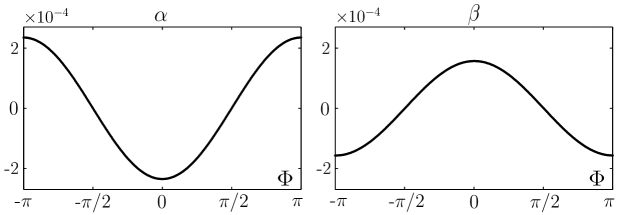
Figure 3: Dependence of $\alpha$ and $\beta$ on $\Phi$ in the case $m$:$n$ = 3:2 with physical parameters (in cgs units): $\rho=1$, $\nu=0.1$, $\Gamma=21.5$, and $\omega=10$, corresponding to $\gamma\simeq 2.08\!\times\!10^{-4}$. To change $\Phi$ we set $\phi_{n}=0$ and varied $\phi_{m}$.

Observe that $\alpha(\Phi)$ and $\beta(\Phi)$ have the opposite phase, i.e., $\alpha\beta<0$, as predicted by the arguments of Section 2.3.1. Maximal values of $|\alpha|$ and $|\beta|$ are realized (for small $\gamma$) when $\Phi=0$. We use such an “optimal” choice of phases, e.g., $\phi_{m}=-\pi/4$ and $\phi_{n}=0$, to test in Fig. 4

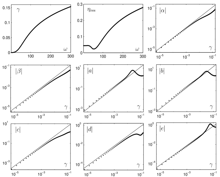
Figure 4: Behavior of $\gamma(\omega)$, $\eta_{\rm res}(\omega)$ (see Eq. (40)), and the magnitude of the coefficients $|\alpha(\gamma)|$, $\dots$, $|e(\gamma)|$ of Eqs. (29-31) over the interval $\omega\in[3,300]$ rad/s with $\phi_{m}=-\pi/4$, $\phi_{n}=0$, $\rho=1$, $\nu=0.1$, and $\Gamma=21.5$ (cgs units). The straight lines show the predicted (linear) $\gamma$ dependence. In the calculation of $\eta_{\rm res}$ we use $\epsilon_{0}=0.1$.

the scalings predicted by Eqs. (32). Note that, as expected for $m$:$n$ = 3:2, we find $\eta_{\rm res}\sim 0.02$–0.3, and resonance effects are likely to be important over much of the weakly nonlinear regime.

For values of $\Phi$ near $\pm\pi/2$, the $\gamma$ dependence of $\alpha$ and $\beta$ switches from the exponent $(m+n-3)/2$, characteristic of the terms given in Eqs. (32), to the exponent $(n+m-1)/2$, reflecting the next nonvanishing term (not calculated). Fig. 5 illustrates this second type of behavior by showing

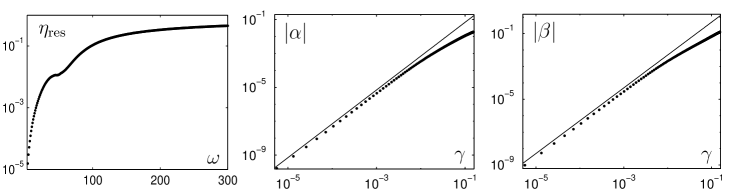
Figure 5: Dependence of $\eta_{\rm res}(\omega)$ (using $\epsilon_{0}=0.1$), $|\alpha(\gamma)|$, and $|\beta(\gamma)|$ when $\Phi=\pi/2$. Parameters are the same as in Fig. 4 except with $\phi_{m}=\pi/4$. Straight lines show the predicted $\gamma^{2}$ dependence.

$\eta_{\rm res}(\omega)$, $|\alpha(\gamma)|$, and $|\beta(\gamma)|$ when $\Phi=\pi/2$. The remaining coefficients in Eqs. (29-31) are essentially unchanged from Fig. 4. Note that $\eta_{\rm res}\rightarrow 0$ as $\omega\rightarrow 0$ (i.e., $\gamma\rightarrow 0$), indicating that resonance effects are becoming increasingly weak – larger values of $\omega$ are required to see them more easily. Furthermore, besides the fact that $\alpha$ and $\beta$ are smaller, we find that $\alpha\beta>0$ over the calculated range $\omega\in[3,300]$. This is in sharp contrast to the typical case, with $\Phi$ bounded away from $\pm\pi/2$, when the leading order terms given in Eqs. (32) dominate and $\alpha\beta<0$. Because the relative phase $\phi_{f}$ (equivalently, $\Phi$) can alter the sizes of $\alpha$ and $\beta$ and the sign of their product, it can have a dramatic effect on the dynamics of resonant triads, as shown in the following section.

4 Dynamics

In this section we discuss the dynamics of Eqs. (29-31) with an eye to the influence of relations (32) and (36). As shown by Guckenheimer and Maholov [35] these dynamics can be very rich, in part because a number of solutions drift or “travel” on the slow time scale, as discussed in Section 2.3.2. In the following we refer to these as drifting waves (DW) to emphasize that this motion is much slower than the fast (standing) oscillations associated with the parametric forcing.

While the temporal symmetries are now implicit, expressed in relations (32) and (36) describing the scaling, parameter-dependence, and relative sign of the SW normal form coefficients, the unbroken spatial symmetries (37-38) force the existence of dynamically invariant subspaces containing distinct classes of solutions; the most important of these fixed point subspaces are listed in Table 1.

Subspace	Fixed by	Defining property
${\cal U_{R}}$	$\cal{R}$	${\rm Im}(A_{j})=0$
${\cal U}_{\kappa}$	$\kappa$	$A_{1}=A_{2}$
${\cal U}_{1}$	${\cal T}_{(0,\phi)}$	$A_{2}=A_{3}=0$
${\cal U}_{2}$	${\cal T}_{(\phi,0)}$	$A_{1}=A_{3}=0$
${\cal U}_{3}$	$\kappa$, ${\cal T}_{(\phi,-\phi)}$	$A_{1}=A_{2}=0$

Table 1: Invariant subspaces of Eqs. (29-31).

Not all of these subspaces are isolated and independent. For example, $\cal{U_{R}}$ contains the solutions that are invariant under inversion through the origin (i.e., under ${\cal R}$) but there is a torus of equivalent subspaces generated by ${\cal T}_{\boldsymbol{\phi}}$; each of these related subspaces is invariant under inversion through an appropriate (translated) origin. Similarly, there is a circle of subspaces equivalent to ${\cal U}_{\kappa}$ generated by ${\cal T}_{(\phi,-\phi)}$; solutions in these subspaces satisfy $A_{2}=e^{i2\phi}A_{1}$ and are reflection-symmetric about a line parallel to $\boldsymbol{k_{3}}$. The subspaces ${\cal U}_{1}$ and ${\cal U}_{2}$ are related by the symmetry $\kappa$ and are equivalent. In the following we use ${\cal U_{R}}$, ${\cal U}_{\kappa}$, and ${\cal U}_{1}$ to denote the entire family of equivalent subspaces, the representative members of which are listed in Table 1. In practice, the most important subspaces are ${\cal U_{R}}$ and ${\cal U}_{\kappa}$ because they relate to easily recognizable characteristics: solutions in ${\cal U_{R}}$ are strictly standing (i.e., they do not drift; see below) while solutions in ${\cal U}_{\kappa}$ possess a line of symmetry and may drift only in a direction parallel (or antiparallel) to $\boldsymbol{k_{3}}$.

For most purposes it helps to factor out the continuous translation symmetry ${\cal T}_{\boldsymbol{\phi}}$ by writing $A_{j}=a_{j}e^{i\theta_{j}}$ and introducing the ${\cal T}_{\boldsymbol{\phi}}$-invariant phase $\theta=\theta_{3}-\theta_{1}-\theta_{2}$. One then obtains the four-dimensional system

$$\dot{r}_{1} =\lambda r_{1}+\alpha r_{2}r_{3}\cos\theta+r_{1}(ar_{1}^{2}+br_{2}^{2}+cr_{3}^{2}),$$ (50)

$$\dot{r}_{2} =\lambda r_{2}+\alpha r_{1}r_{3}\cos\theta+r_{2}(ar_{2}^{2}+br_{1}^{2}+cr_{3}^{2}),$$ (51)

$$\dot{r}_{3} =\mu r_{3}+\beta r_{1}r_{2}\cos\theta+r_{3}(dr_{1}^{2}+dr_{2}^{2}+er_{3}^{2}),$$ (52)

$$\dot{\theta} =-\big{(}\beta\,\frac{r_{1}r_{2}}{r_{3}}+\alpha\frac{r_{2}r_{3}}{r_{1}}+\alpha\frac{r_{1}r_{3}}{r_{2}}\big{)}\sin\theta,$$ (53)

where the $\theta_{j}$ satisfy

$$\dot{\theta_{1}}=\alpha\frac{r_{2}r_{3}}{r_{1}}\sin\theta,\qquad\dot{\theta_{2}}=\alpha\frac{r_{1}r_{3}}{r_{2}}\sin\theta,\qquad\dot{\theta_{3}}=-\beta\frac{r_{1}r_{2}}{r_{3}}\sin\theta.$$ (54)

Eqs. (54) guarantee that solutions in ${\cal U_{R}}$, which corresponds to $\{\theta=0\}$ $\cup$ $\{\theta=\pi\}$ in Eqs. (50-53), are also standing (i.e., all phase velocities are zero). Furthermore, from Eq. (53) it follows that unless $\alpha\beta<0$ the quantity multiplying $\sin\theta$ is single-signed and all trajectories approach ${\cal U_{R}}$ (see [35, 36]), i.e., there are no permanently drifting solutions if $\alpha\beta>0$. The fact that one can expect drifting solutions on the basis of underlying Hamiltonian structure was the conclusion of Section 2.3.1

4.1 Principal solutions

We describe here the most important solutions of Eqs. (29-31), equivalently, Eqs. (50-52). Many of these solutions (or their analogs) are discussed in [35]. They are summarized, along with the bifurcations they undergo, in Table 2.

Table 2: Typical solutions (see text) classified according to the reflection symmetries ${\cal R}$ and $\kappa$. Broken lines indicate potential bifurcations.

(1) Standing rolls SR₁ $\in$ ${\cal U}_{1}$

The SR₁ states satisfy $|A_{1}|^{2}=-\lambda/a$, $A_{2}=A_{3}=0$. Physically, they represent SW with dominant frequency $m/2$ described by a single wavevector ${\boldsymbol{k}}_{1}$. Standing rolls SR₂ with wavevector ${\bf k}_{2}$ are related to SR₁ through the symmetry $\kappa$ and are equivalent. Both bifurcate from the flat state (O) when $\lambda=0$, supercritically if $a<0$. The eigenvalues of SR₁ within the two-dimensional subspace ${\cal U}_{1}$ are 0 (a result of the translational symmetry ${\cal T}_{\boldsymbol{\phi}}$) and $-2\lambda$. Transverse to ${\cal U}_{1}$ the eigenvalues $\xi$ have multiplicity two and satisfy

$$a^{2}\xi^{2}-a\left(a\mu+\lambda(a-b-d)\right)\xi+\lambda(a-b)(a\mu-d\lambda)+a\beta\lambda=0.$$ (55)

Near onset (i.e., $|\lambda|\ll$ 1) these eigenvalues are approximated by $\mu$ and $\lambda(a-b+\alpha\beta/\mu)/a$. Thus, the standing rolls SR₁ are stable at onset if $a<0$ (the bifurcation is supercritical), $\mu<0$ (stability with respect to perturbations of type $A_{3}$ is inherited from the basic flat state), and $\mu(b-a)>\alpha\beta$; they are unstable otherwise.

The SR₁ states undergo a steady-state bifurcation along the line

$$\mu=\frac{\alpha\beta}{b-a}+\frac{d}{a}\,\lambda,$$ (56)

giving rise to a branch of mixed modes (MM) contained in ${\cal U_{R}}$ with $A_{2}\neq 0$, $A_{3}\neq 0$, and experience a Hopf bifurcation along the line

$$\mu=\frac{b+d-a}{a}\,\lambda,$$ (57)

provided $\alpha\beta<\lambda(a-b)^{2}/a<0$. This Hopf bifurcation with $O(2)$ symmetry (see, e.g., [18])) simultaneously produces modulated standing waves (MSW) contained in ${\cal U_{R}}$, and DW not in ${\cal U_{R}}$. Note that $\alpha\beta<0$ is a necessary condition for this bifurcation, as it must be if DW are produced. Assuming this condition holds, the line of Hopf bifurcations (57) intersects the line of steady bifurcations (56) at the Takens-Bogdanov point: $(\lambda,\mu)=\alpha\beta(a,b+d-a)/(b-a)^{2}$.

(2) Standing Rolls SR₃ $\in$ ${\cal U}_{3}$.

The SR₃ states satisfy $A_{1}=A_{2}=0$, $|A_{3}|^{2}=-\mu/e$ and represent harmonic SW (dominant frequency $n/2$) with wavevector ${\boldsymbol{k}}_{3}$. They bifurcate from O when $\mu=0$, supercritically if $e<0$. Within ${\cal U}_{3}$ the eigenvalues are 0 and $-2\mu$ while the remaining four eigenvalues come in pairs given by

$$s=\lambda-\frac{c}{e}\mu\pm\alpha\sqrt{\frac{-\mu}{e}}.$$ (58)

In contrast to SR₁, only steady-state bifurcations can occur on SR₃ and these generate branches of mixed modes MM_κ $\in$ ${\cal U}_{\kappa}$ (i.e., the unstable eigenvectors satisfy $|A_{1}|=|A_{2}|$).

(3) $\kappa$-symmetric mixed modes MM_κ $\in$ ${\cal U_{R}}$ $\cap$ ${\cal U}_{\kappa}$ .

These mixed modes bifurcate, along with SR₁, from O when $\lambda=0$. The ${\cal T}_{\boldsymbol{\phi}}$-invariant phase $\theta$ must be 0 or $\pi$ while the amplitudes satisfy

$$(2cd-(a+b)e)r_{3}^{3}\pm(2\alpha d+\beta c)r_{3}^{2}+(2d\lambda+\alpha\beta-(a+b)\mu)r_{3}\pm\beta\lambda=0,$$

$$r_{1}^{2}=r_{2}^{2}=-\frac{cr_{3}^{2}\pm\alpha r_{3}+\lambda}{a+b},$$ (59)

with $\cos\theta$ dictating the $\pm$ sign. Eqs. (59) show that there can be up to three distinct MM_κ states for each of the two possible $\theta$ values. The additional solutions arise in saddle-node bifurcations, and other transitions can occur as well. Hopf bifurcations lead to modulated standing waves, MSW_κ, still contained in ${\cal U}_{\kappa}$ $\cap$ ${\cal U_{R}}$, while symmetry-breaking bifurcations lead to drifting waves DW_κ $\in$ ${\cal U}_{\kappa}$ (broken ${\cal R}$ symmetry) or to mixed modes MM $\in$ ${\cal U_{R}}$ (broken $\kappa$ symmetry). The MM states bifurcate only from the MM_κ branch with $\cos\theta={\rm sign}(\alpha(a-b))$ and do so when

$$\mu=\frac{\alpha\beta}{b-a}+\frac{e}{c}\lambda+\frac{2\alpha(cd-ae)}{c^{2}(a-b)^{2}}\big{(}a\alpha\pm\sqrt{a^{2}\alpha^{2}-\lambda c(b-a)^{2}}\,\big{)}.$$ (60)

(4) $\kappa$-symmetric drifting waves DW_κ $\in$ ${\cal U}_{\kappa}$.

These solutions require $\alpha\beta<0$. Within Eqs. (29-31) they drift with constant velocity parallel to $\pm{\boldsymbol{k}}_{3}$ (i.e., $\dot{\theta}_{1}=\dot{\theta}_{2}=\dot{\theta}_{3}/2$). Within the four-dimensional reduced system (50-53) they appear as fixed points with $\theta\neq 0$ or $\pi$ satisfying

$$r_{3}^{2}=-\frac{\beta(\mu+2\lambda)}{4\alpha(a+b+d)-\beta(2c+e)},\qquad r_{1}^{2}=r_{2}^{2}=-\frac{2\alpha}{\beta}\,r_{3}^{2},$$

$$r_{3}\cos\theta=\frac{\mu(2\alpha(a+b)-\beta c)+\lambda(\beta e-4\alpha d)}{\alpha(4\alpha(a+b+d)-\beta(2c+e))},$$ (61)

and exist in the region

$$(\mu(2\alpha(a+b)-c\beta)-\lambda(4d\alpha-e\beta))^{2}\leq(\mu+2\lambda)\alpha^{2}(4\alpha\beta(a+b+d)-\beta^{2}(2c+e)).$$ (62)

The DW_κ states themselves can undergo Hopf bifurcations to create modulated drifting waves MDW_κ $\in$ ${\cal U}_{\kappa}$, as well as symmetry-breaking bifurcations to DW not in ${\cal U}_{\kappa}$. This latter bifurcation occurs along the line

$$\mu=\frac{4\alpha(b+d-a)-\beta e}{4\alpha a-\beta c}\,\lambda.$$ (63)

(5) Mixed modes MM $\in$ ${\cal U_{R}}$

These mixed states (without $\kappa$ symmetry) satisfy

$$r_{3}^{2}=\frac{\alpha\beta a+(a\mu-d\lambda)(a-b)}{(a-b)(cd-ae)},\qquad\cos\theta={\rm sign}(\alpha(a-b)),$$

$$r_{1}^{2}+r_{2}^{2}=-\frac{\lambda+cr_{3}^{2}}{a},\qquad r_{1}r_{2}=\left|\frac{\alpha}{a-b}\right|r_{3}.$$ (64)

They form a branch of solutions connecting the SR₁ (SR₂) states with the MM_κ branch having $\cos\theta={\rm sign}(\alpha(a-b))$. There are no saddle-node bifurcations but if $\alpha\beta<0$ there is an ${\cal R}$ symmetry-breaking instability that creates drifting waves DW along the line

$$\mu=\frac{e}{c}\,\lambda+\frac{\alpha\beta(bc+cd-ac-ae)}{c(a-b)^{2}}.$$ (65)

(6) Drifting waves DW.

These steadily drifting solutions (requiring $\alpha\beta<0$) of Eqs. (29-31) are not in ${\cal U}_{\kappa}$ and are therefore free to move in any direction (i.e., their drift direction is determined by the coefficients, not by symmetry). They are represented by fixed points within Eqs. (50-53) satisfying

$$r_{3}^{3}=\frac{a\mu+(a-b-d)\lambda}{bd+cd-ac-ae},\qquad r_{1}^{2}+r_{2}^{2}=-\frac{\lambda+cr_{3}^{2}}{a},$$

$$\cos^{2}\theta=\frac{(a-b)^{2}(\lambda+cr_{3}^{2})}{\alpha\beta a},\qquad r_{1}r_{2}=\frac{\alpha r_{3}\cos\theta}{a-b}.$$ (66)

As with MM (and DW_κ) there are no saddle-node bifurcations. In fact, for the sets of parameters we investigated there were no additional bifurcations on the DW branch.

(7) $\kappa$-symmetric modulated standing waves MSW_κ $\in$ ${\cal U_{R}}$ $\cap$ ${\cal U}_{\kappa}$.

These states appear via Hopf bifurcation from MM_κ. The form of the bifurcation set is nontrivial but reduces to a parabola (see [37, 38]) near the origin $(\mu,\lambda)=(0,0)$:

$$\mu\simeq-\frac{3e}{|\alpha|}\lambda^{2},\qquad\alpha\beta e\lambda<0$$ (67)

The MSW_κ solutions may undergo an ${\cal R}$ symmetry-breaking bifurcation to modulated drifting waves MDW_κ and are typically destroyed in a global bifurcation involving a heteroclinic connection between O and SR₃ (see [36, 39]).

(8) Modulated standing waves MSW $\in$ ${\cal U_{R}}$ .

These solutions do not have the $\kappa$ symmetry of MSW_κ. They appear, along with DW, in a Hopf bifurcation on SR₁.

(9) $\kappa$-symmetric modulated drifting waves MDW_κ $\in$ ${\cal U}_{\kappa}$.

These three-frequency states can emerge from DW_κ through Hopf bifurcation or from MSW_κ via an ${\cal R}$ symmetry-breaking bifurcation.

(10) Heteroclinic cycles HET.

There are (at least) three kinds of heteroclinic cycles of relevance to Eqs. (29-31). Structurally stable heteroclinic cycles (HET₁) connecting two SR₃ solutions, out of phase by $\pi$ (i.e., related by a translation ${\cal T}_{(\phi,\pi-\phi)}$), have been well studied [34, 36] in the context of the 1:2 steady-state spatial resonance with O(2) symmetry and in resonant triads as well [35]. They are generic solutions when $\alpha\beta<0$ that appear at small amplitude ($|\lambda|,|\mu|\ll 1$).

In addition, there are much more intricate heteroclinic cycles (HET₂) involving connections among O, SR₃, MSW_κ, and MM_κ (see [39]). Under appropriate conditions, these cycles form near the HET₁ cycles (in a neighboring region of parameter space but further from the origin). The associated dynamics is organized by a sequence of transitions among distinct heteroclinic cycles (one of which is structurally stable) and contains chaos of Shil’nikov type. The type of chaotic attractor one typically finds is shown in Fig. 6.

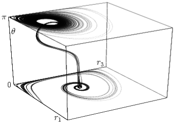
Figure 6: Chaotic attractor in Eqs. (50-53) obtained at $(\lambda,\mu)=(-0.0377,0.035)$ with the coefficients $\alpha=-0.19$, $\beta=0.166$, $a=-0.0399$, $b=-0.436$, $c=1.27$, $d=-1.43$, and $e=-0.106$, derived from the Zhang-Viñals model (41) with $m$:$n=1$:2, $\Phi=\pi/4$, and (in cgs units) $\omega=200$, $\nu=0.01$, $\Gamma=70$. This attractor is in ${\cal U}_{\kappa}$ and visits the neighborhood of two MM_κ fixed points: one with $\theta=0$ and one with $\theta=\pi$. The latter is near a Hopf bifurcation to MSW_κ. The boundary $r_{3}=0$ should be identified at $\theta=0$ and $\theta=\pi$.

When the resonance terms vanish (i.e., at $\alpha=\beta=0$) there are, under certain conditions [35], heteroclinic cycles connecting SR₁, SR₂, and SR₃. Because of the resonant terms in Eqs. (29-31) these cycles are no longer present. Nonetheless, for large $m+n$ when resonance effects are diminished, or at values of $\phi_{m}$ and $\phi_{n}$ where $\Phi=\pm\pi/2$ and the leading order resonant term vanishes (see Eqs. (32)), these “nearby” cycles may yet exert an influence on the dynamics.

4.2 Bifurcations: numerical examples

We provide here some numerical examples using coefficients derived from the Zhang-Viñals equations (41). Figure 7 shows the bifurcations that occur for

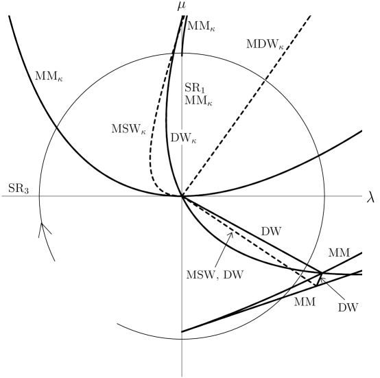
Figure 7: Bifurcation sets for the case $m$:$n=1$:2 and $\Phi=0$ with (in cgs units) $\rho=1$, $\nu=0.1$, $\Gamma=21.5$, and $\omega=200$. Curves are labelled by the solutions generated (see text) and are dashed in the case of Hopf bifurcation. The clockwise circular path is used to generate the bifurcation diagram in Fig. 8 and is at a radius $\sqrt{\lambda^{2}+\mu^{2}}=0.0128$.

$m$:$n=1$:2, $\Phi=0$, $\rho=1$, $\nu=0.1$, $\Gamma=21.5$, and $\omega=200$ (cgs units); for these parameters $\gamma=0.0341$ and we find $\alpha=-0.265$, $\beta=0.281$, $a=-6.136$, $b=0.0266$, $c=-0.98$, $d=-2.076$, and $e=-2.234$. We use $m$:$n=1$:2 rather that $m$:$n=3$:2 (as in Section 3) mainly for pedagogical reasons: although the bifurcations seen with other forcing ratios such as 3:2 (and comparable physical parameters) are the same as those found in Fig. 7 they tend to be somewhat more bunched together thus more difficult to illuminate. The use of 1:2 forcing also has the advantage of the large ${\cal O}(1/\gamma)$ oscillations with $\Phi$ in $b$, $c$, and $d$ (see Eqs. (32)); this leads to greater control over the normal form coefficients and hence to a wider range of dynamical possibilities (for example, this $\Phi$-dependence made it easier to find the interesting heteroclinic behavior shown in Fig. 6).

If one traverses the clockwise circular path shown in Fig. 7 the resulting bifurcation diagram is that of Fig. 8. Initially, in the third quadrant

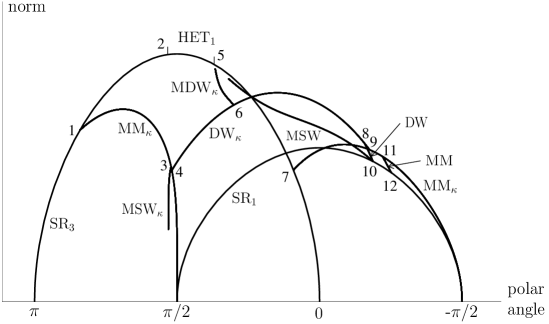
Figure 8: Bifurcation diagram for the clockwise circular path shown in Fig. 7

of the $(\lambda,\mu)$ plane, all initial conditions are attracted to the stable flat state O. As the polar angle ($\phi$, say) is decreased through $\pi$ this flat state becomes unstable to (a circle of) standing rolls of type SR₃. At $\phi\simeq 2.64$ (point 1 in Fig. 8) these stable SR₃ states in turn undergo a supercritical symmetry-breaking bifurcation to (a torus of) $\kappa$-symmetric mixed modes MM_κ satisfying $\theta=\pi$. These MM_κ states are stable until a subcritical Hopf bifurcation at $\phi\simeq 1.64$ (point 3) producing $\kappa$-symmetric modulated standing waves MSW_κ. The MSW_κ are themselves destroyed in a heteroclinic bifurcation (point 2, marked by a small dash on the SR₃ branch) joining O and SR₃ (see [39]) at $\phi\simeq 1.67$. The same global bifurcation marks the birth of structurally (and asymptotically) stable heteroclinic cycles (HET₁) connecting points on the circle of SR₃ states to their “$\pi$ translates”. After the Hopf bifurcation renders MM_κ unstable the heteroclinic cycles HET₁ are the only attractors of the system (29-31). These HET₁ remain stable until $\phi\simeq 1.16$ (point 5; this is when $\mu=\lambda e/c$ and the two eigenvalues of Eq. (58), one positive and one negative, are of equal magnitude). The bifurcation that occurs here simultaneously produces stable MDW_κ and unstable MSW (the fact that the MSW branch does not visibly originate here is due to numerical limitations). The stable MTW_κ branch describes modulations of ever decreasing amplitude as it approaches the branch of DW_κ states, themselves present since an ${\cal R}$ symmetry-breaking bifurcation on MM_κ at $\phi\simeq 1.63$ (point 4), and is destroyed in a Hopf bifurcation at $\phi\simeq 0.95$ (point 6). The DW_κ are then stable until a supercritical $\kappa$ symmetry-breaking bifurcation to DW at $\phi\simeq-0.5$ (point 8); this occurs just prior to their termination at $\phi\simeq-0.55$ (point 9) on the other MM_κ branch, i.e., the one with $\theta=0$ existing between $\phi=-\pi/2$ and a bifurcation from SR₃ at $\phi\simeq 0.29$ (point 7). The stable DW branch terminates, along with the unstable MSW branch, in a Hopf bifurcation on SR₁ at $\phi\simeq-0.59$ (point 10). The SR₁ rolls are stable between this Hopf bifurcation and a subcritical bifurcation to MM at $\phi\simeq-0.79$ (point 12). This MM branch also connects to (and stabilizes) the MM_κ branch at $\phi\simeq-0.7$ (point 11). Finally, the MM_κ states (with $\theta=0$) are stable between this last bifurcation and $\phi=-\pi/2$ where they vanish, along with SR₁, restoring stability to the flat state.

If, in contrast to the case of Fig. 7, one adjusts the forcing phases so that $\Phi=\pi/2$ then the (leading order) expressions for $\alpha$ and $\beta$ of Eqs. (32) vanish. With the same physical parameters as Fig. 7 it turns out that the first nonvanishing contributions have the same algebraic sign, i.e., $\alpha\beta>0$. Specifically, we find $\alpha=0.0784$, $\beta=0.0744$, $a=0.549$, $b=-0.523$, $c=-0.0155$, $d=-3.266$, and $e=-2.227$. The fact that $\alpha\beta>0$ explains the dramatically different (and less rich) unfolding shown in Fig. 9. In this case

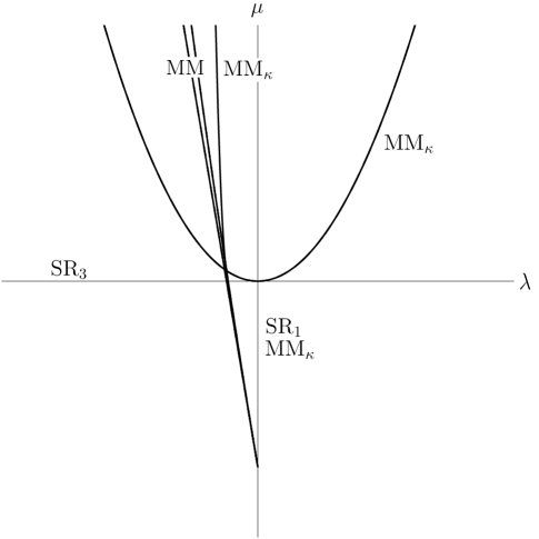
Figure 9: Bifurcation sets for $m$:$n=1$:2 with the same parameters as Fig. 7 except that $\Phi=\pi/2$. For this choice of phase $\alpha\beta>0$ and there are no DW_κ, MDW_κ, DW, MSW_κ, MSW, or heteroclinic solutions.

there are no drifting solutions (DW_κ, MDW_κ, DW) or heteroclinic cycles (HET₁, HET₂). Furthermore, there are no modulated standing waves MSW_κ or MSW (in was shown in [37] that $\alpha\beta<0$ is necessary for MSW_κ). A second, somewhat surprising, feature of the $\Phi=\pi/2$ coefficients is the large change in the self-interaction coefficient $a$: it is now positive whereas at $\Phi=0$ it was $-6.136$. Such substantial $\Phi$-dependence is not an ingredient of Eqs. (32) and is a result of “1:2” linear resonances, i.e., harmonic modes satisfying $\boldsymbol{k}=2\boldsymbol{k}_{1}$ or $\boldsymbol{k}=2\boldsymbol{k}_{2}$. The influence of these damped modes (see [10]) is especially strong here because $k_{3}\approx 1.86$ is quite close to $2k_{1}\approx 1.94$ (the damping of the $2k_{1}$ modes is thus very small and they nearly satisfy the 1:2 temporal resonance condition $m=\Omega(2k_{1})$; in this case $m=n/2$). For comparison, note that the $2k_{3}$ modes are not “almost” neutral and the corresponding self-interaction coefficient $e$ shows no significant dependence on $\Phi$, in agreement with Eqs. (32). Because $a>0$ the bifurcation of SR₁ and MM_κ from the flat state is now subcritical (observe how the MM bifurcations from SR₁ and MM_κ have switched to the left side of $\lambda=0$ in Fig. 9) and the cubic truncation (29-31) is no longer well-behaved (some trajectories diverge).

5 Conclusions

The weakly nonlinear dynamics of a class of resonant triads occurring in the vicinity of the bicritical point of the two-frequency forced Faraday problem has been studied in detail. The approach taken for this resonant triad can be easily extended to a wide range of patterns produced by multi-frequency forcing (see [9]), and is based on very general symmetry considerations. In particular, we make use of the fact that the weakly damped problem possesses additional structure beyond the more obvious spatial and discrete temporal symmetries, i.e., it must satisfy the constraints of continuous time translation and time reversal (when these are viewed as parameter symmetries) and respect the nearby Hamiltonian structure of the undamped problem. The effect of these “broken” symmetries is straightforward to establish in the context of TW equations (17-18), and in the reduced SW equations (29-31) reveals itself in the structure of the normal form coefficients (32). Most notably, we found that the SW coefficients of the quadratic resonance terms ($\alpha$ and $\beta$) could be expected to be of opposite sign, exhibit simple harmonic dependence on the phase $\Phi$, and scale as the damping $\gamma$ to the power $(m+n-3)/2$. Each of these predictions was supported in the direct numerical calculation of coefficients from the Zhang-Viñals equations (41). Moreover, the exponential decrease in the size of the resonance terms with $m+n$ provides an explanation for the lack of experimental observations [3, 8] of this triad with large values of $m$ and $n$. Recall, however, that this simple prediction (as well as the other scaling laws) emerged after we expanded the SW normal form coefficients in powers of $f_{m}$, $f_{n}$, and $\gamma$ (see Eqs. (19-23)). Particularly in the case of $\gamma$ it is not clear that the assumption of analyticity is a good one – the addition of damping is known to act as a singular perturbation (see, e.g., [40, 41]). For the quasipotential equations of Zhang and Viñals the numerical agreement (and hence the justification for a simple Taylor expansion) is quite convincing, but we speculate that a more rigorous treatment using the Navier-Stokes equations with realistic boundary conditions and finite fluid depth may lead to a departure, in some regimes, from the scalings given here. This departure will presumably be small in weakly damped systems of large depth where the Zhang-Viñals equations are expected to be valid.

The resonant triad system (29-31) exhibits extremely rich dynamics, much more so in the case where the resonant coefficients satisfy $\alpha\beta<0$. That the underlying Hamiltonian structure makes this the typical case for weak damping and, furthermore, that this situation depends on the relative phase of the two forcing terms, is a result we have emphasized throughout this paper. When $\alpha\beta<0$ there exist several types of modulated standing waves, drifting waves (of both steady and modulated character), and heteroclinic cycles with associated phenomena like the chaotic attractor of Fig. 6. It must be admitted, however, that none of these more complicated solutions has yet been reported in the experimental literature; other than simple roll states, only the mixed mode MM_κ has been established experimentally [8]. It is quite possible that the remaining solutions are simply unstable when all types of perturbations are considered (the system may prefer hexagons or squares, for example). It might also be that the use of finite containers plays a critical role in preventing many of these solutions from appearing (the drifting waves DW_κ, DW, and MTW_κ obviously cannot exist as such in nonperiodic bounded domains). It would be interesting to see if a more deliberate search, perhaps in a very large aspect ratio container, would reveal more features of the dynamics presented in Section 4. On the other hand, it would miss the point to focus too narrowly on the resonant triad treated here. This paper is also intended to serve as a detailed illustration of a very general method with wide applicability to parametrically forced problems, particularly those with forcing functions composed of multiple frequencies – for example, in [9] we considered two-frequency forced hexagons and two-mode superlattices [5]. The symmetry-based approach of this paper provides, for weakly damped systems, a means of determining scaling laws and other important qualitative features of the normal form coefficients without resorting to a full center manifold reduction from the governing equations (often an exceedingly difficult task). The results also suggest how one might begin to think about designing forcing functions that enhance, suppress, or otherwise control the patterns of interest (superlattices, for example). This very intriguing direction will be pursued in future work [42].

Appendix A Appendix

We give here the expressions for $J_{1},...,J_{7}$ appearing in Eqs. (32).

$$J_{1}=\frac{2\varrho_{r}^{2}}{\tilde{\mu}_{i}^{2}}\big{(}\hat{\upsilon}_{n}+\frac{\upsilon_{r}\tilde{\lambda}_{n}}{\tilde{\lambda}_{i}}-\upsilon_{n}C_{1}\big{)},\quad\;{\rm where}\quad C_{1}=\frac{\upsilon_{\gamma}}{\upsilon_{r}}+\frac{\upsilon_{m}\upsilon_{r}}{\tilde{\lambda}_{i}^{2}}+\frac{\upsilon_{n}\varrho_{r}^{2}}{\upsilon_{r}\tilde{\mu}_{i}^{2}},$$ (68)

$$J_{2}=\frac{2\upsilon_{r}^{2}}{\tilde{\lambda}_{i}^{2}}\big{(}\hat{\varrho}_{m}+\frac{\varrho_{r}\tilde{\mu}_{m}}{\tilde{\mu}_{i}}-\varrho_{n}C_{2}\big{)},\quad{\rm where}\quad C_{2}=\frac{\varrho_{\gamma}}{\varrho_{r}}+\frac{\varrho_{m}\upsilon_{r}^{2}}{\varrho_{r}\tilde{\lambda}_{i}^{2}}+\frac{\varrho_{n}\varrho_{r}}{\tilde{\mu}_{i}^{2}},$$ (69)

$$J_{3}={\rm a}_{r}+{\rm b}_{r}-C_{1}({\rm a}_{i}+{\rm b}_{i})+\frac{\upsilon_{r}}{\tilde{\lambda}_{i}}\big{(}({\rm r}_{2})_{i}-({\rm q}_{1})_{i}-({\rm q}_{2})_{i}\big{)},$$ (70)

$$J_{4}=\delta_{r}+{\rm c}_{r}+{\rm d}_{r}-C_{1}(\delta_{i}+{\rm c}_{i}+{\rm d}_{i})+\frac{\upsilon_{r}}{\tilde{\lambda}_{i}}\big{(}({\rm r}_{3})_{i}-({\rm r}_{1})_{i}-({\rm q}_{3})_{i}-({\rm q}_{4})_{i}\big{)},$$ (71)

$$J_{5}={\rm e}_{r}+{\rm f}_{r}-C_{1}({\rm e}_{i}+{\rm f}_{i})-\frac{\upsilon_{r}}{\tilde{\lambda}_{i}}\big{(}({\rm q}_{5})_{i}+({\rm q}_{6})_{i}\big{)}+\frac{\varrho_{r}}{\tilde{\mu}_{i}}\big{(}({\rm r}_{5})_{i}-({\rm r}_{4})_{i}\big{)},$$ (72)

$$J_{6}={\rm g}_{r}+{\rm h}_{r}-C_{2}({\rm g}_{i}+{\rm h}_{i})-\frac{\varrho_{r}}{\tilde{\mu}_{i}}\big{(}({\rm s}_{1})_{i}+({\rm s}_{2})_{i}\big{)}+\frac{\upsilon_{r}}{\tilde{\lambda}_{i}}\big{(}({\rm u}_{2})_{i}-({\rm u}_{1})_{i}\big{)},$$ (73)

$$J_{7}={\rm l}_{r}+{\rm p}_{r}-C_{2}({\rm l}_{i}+{\rm p}_{i})+\frac{\varrho_{r}}{\tilde{\mu}_{i}}\big{(}({\rm u}_{3})_{i}-({\rm s}_{3})_{i}-({\rm s}_{4})_{i}\big{)}.$$ (74)

References

- [1] M. Faraday, On the forms and states of fluids on vibrating elastic surfaces, Phil. Trans. R. Soc. Lond. 121 (1831) 319–340.
- [2] D. Binks, W. van de Water, Nonlinear pattern formation of Faraday waves, Phys. Rev. Lett. 78 (1997) 4043–4046.
- [3] H. Arbell, J. Fineberg, Pattern formation in two-frequency forced parametric waves, Phys. Rev. E 65 (2002) 036224.
- [4] W. S. Edwards, S. Fauve, Patterns and quasi-patterns in the Faraday experiment, J. Fluid Mech. 278 (1994) 123–148.
- [5] H. Arbell, J. Fineberg, Spatial and temporal dynamics of two interacting modes in parametrically driven surface waves, Phys. Rev. Lett. 81 (1998) 4384–4387.
- [6] A. Kudrolli, B. Pier, J. P. Gollub, Superlattice patterns in surface waves, Physica D 123 (1998) 99–111.
- [7] T. B. Benjamin, F. Ursell, The stability of a plane free surface of a liquid in vertical periodic motion, Proc. Roy. Soc. London A 225 (1954) 505–515.
- [8] H. Arbell, J. Fineberg, Two-mode rhomboidal states in driven surface waves, Phys. Rev. Lett. 84 (2000) 654–657.
- [9] J. Porter, M. Silber, Broken symmetries and pattern formation in two-frequency forced Faraday waves, Phys. Rev. Lett. 89 (2002) 084501.
- [10] C. M. Topaz, M. Silber, Resonances and supperlattice pattern stabilization in two-frequency forced Faraday waves, Physica D 172 (2002) 1–29.
- [11] M. Silber, A. C. Skeldon, Parametrically excited surface waves: Two-frequency forcing, normal form symmetries and pattern formation, Phys. Rev. E 59 (1999) 5446–5456.
- [12] H. W. Müller, Periodic triangular patterns in the Faraday experiment, Phys. Rev. Lett. 71 (1993) 3287–3290.
- [13] C. Wagner, H. W. Müller, K. Knorr, Crossover from a square to a hexagonal pattern in Faraday surface waves, Phys. Rev. E 62 (2000) R33–R36.
- [14] W. Zhang, J. Viñals, Pattern formation in weakly damped parametric surface waves, J. Fluid Mech. 336 (1997) 301–330.
- [15] W. Zhang, J. Viñals, Pattern formation in weakly damped parametric surface waves driven by two frequency components, J. Fluid Mech. 341 (1997) 225–244.
- [16] M. Silber, C. M. Topaz, A. C. Skeldon, Two-frequency forced Faraday waves: weakly damped modes and pattern selection, Physica D 143 (2000) 205–225.
- [17] S. T. Milner, Square patterns and secondary instabilities in driven capillary waves, J. Fluid Mech. 225 (1991) 81–100.
- [18] M. Golubitsky, I. Stewart, D. G. Shaeffer, Singularities and Groups in Bifurcation Theory, Volume 2, Springer-Verlag, New York, 1988.
- [19] J. D. Crawford, E. Knobloch, Symmetry and symmetry-breaking bifurcations in fluid mechanics, Annu. Rev. Fluid Mech. 23 (1991) 341–387.
- [20] H. Riecke, J. D. Crawford, E. Knobloch, Time-modulated oscillatory convection, Phys. Rev. Lett. 61 (1988) 1942–1945.
- [21] H. Riecke, M. Silber, L. Kramer, Temporal forcing of small-amplitude waves in anisotropic systems, Phys. Rev. E 49 (1994) 4100–4113.
- [22] J. W. Swift, Hopf bifurcation with the symmetry of the square, Nonlinearity 1 (1988) 333–377.
- [23] W. Zhang, Pattern formation in weakly damped parametric surface waves, Ph.D. thesis, Florida State University (1994).
- [24] J. D. Crawford, Introduction to bifurcation-theory, Rev. Mod. Phys. 63 (1991) 991–1037.
- [25] K. Kumar, L. S. Tuckerman, Parametric instability of the interface between two fluids, J. Fluid Mech. 279 (1994) 49–68.
- [26] V. E. Zakharov, Stability of periodic waves of finite amplitude on the surface of deep fluid, J. Appl. Mech. Tech. Phys. 2 (1968) 190–194.
- [27] J. W. Miles, On Hamilton’s principle for surface waves, J. Fluid Mech. 83 (1977) 153–158.
- [28] L. J. F. Broer, On the Hamiltonian theory of surface waves, Appl. Sci. Res. 29 (1974) 430–446.
- [29] P. Lyngshansen, P. Alstrom, Perturbation theory of parametrically driven capillary waves at low viscosity, J. Fluid Mech. 351 (1997) 301–344.
- [30] A. C. Radder, An explicit Hamiltonian formulation of surface waves in water of finite depth, J. Fluid Mech. 237 (1992) 435–455.
- [31] J. W. Miles, Nonlinear Faraday resonance, J. Fluid Mech. 146 (1984) 285–302.
- [32] V. P. Krasitskii, On reduced equations in the Hamiltonian theory of weakly nonlinear surface waves, J. Fluid Mech. 272 (1994) 1–20.
- [33] P. Chossat, The bifurcation of heteroclinic cycles in systems of hydrodynamical type, Dynam. Cont. Dis. Ser. A 8 (2001) 575–590.
- [34] C. A. Jones, M. R. E. Proctor, Strong spatial resonance and traveling waves in Benard convection, Phys. Lett. A 121 (1987) 224–228.
- [35] J. Guckenheimer, A. Mahalov, Resonant triad interactions in symmetric systems, Physica D 54 (1992) 267–310.
- [36] D. Armbruster, J. Guckenheimer, P. Holmes, Heteroclinic cycles and modulated traveling waves in systems with O(2) symmetry, Physica D 29 (1988) 257–282.
- [37] G. Dangelmayr, Steady-state mode interactions in the presence of O(2)-symmetry, Dynam. Stabil. Syst. 1 (1986) 159–185.
- [38] M. R. E. Proctor, C. A. Jones, The interaction of two spatially resonant patterns in thermal convection. Part 1. Exact 1:2 resonance, J. Fluid Mech. 188 (1988) 301–335.
- [39] J. Porter, E. Knobloch, New type of complex dynamics in the 1:2 spatial resonance, Physica D 159 (2001) 125–154.
- [40] O. M. Phillips, The Dynamics of the upper Ocean, Cambridge Univ. Press, Cambridge, 1977.
- [41] C. Martel, E. Knobloch, Damping of nearly inviscid water waves, Phys. Rev. E 56 (1997) 5544–5548.
- [42] J. Porter, C. M. Topaz, M. Silber, Faraday wave pattern selection via multi-frequency forcing, work in progress.