Emergence of a complex and stable network in a model ecosystem with extinction and mutation

Abstract

We propose a minimal model of the dynamics of diversity — replicator equations with extinction, invasion and mutation. We numerically study the behavior of this simple model and show that it displays completely different behavior from the conventional replicator equation and the generalized Lotka-Volterra equation. We reach several significant conclusions as follows: (1) a complex ecosystem can emerge when mutants with respect to species-specific interaction are introduced; (2) such an ecosystem possesses strong resistance to invasion; (3) a typical fixation process of mutants is realized through the rapid growth of a group of mutualistic mutants with higher fitness than majority species; (4) a hierarchical taxonomic structure (like family-genus-species) emerges; and (5) the relative abundance of species exhibits a typical pattern widely observed in nature. Several implications of these results are discussed in connection with the relationship of the present model to the generalized Lotka-Volterra equation.

and

1 Introduction

The relationship between the complexity and stability of an ecosystem has been one of the most fascinating topics in theoretical biology for decades (Pimm 1991). In the 1950s and 1960s the proposition that highly complex communities are more stable than simple ones was widely supported (MacArther, 1955; Elton, 1958). However, this view was challenged by theorists in the 1970s, who discussed the stability of a community of species interacting randomly (Gardner & Ashby, 1970; May, 1972, 1974; Roberts, 1974; Gilpin & Case, 1976; Taylor, 1988a). The most significant result was given by May (1972), who considered a large-dimensional ecological equation with an $n$-dimensional random interaction matrix $\{a_{ij}\}$ whose diagonal elements are $-1$ and whose off-diagonal elements are assigned as Gaussian random numbers with mean $0$ and variance $\alpha^{2}$ (with probability $C$) or $0$ (with probability $1-C$). He found a kind of phase transition from stability to instability in which the equilibrium solution corresponding to the coexistence of all species becomes unstable if $\alpha>(nC)^{-1/2}$. He concluded that an ecological system cannot be stable if it is complex. After May’s work and the clear conclusions he reached, a number of mathematical biologists attempted to explain the discrepancy between the observed complexity of ecosystems in nature and the results of these mathematical studies. Their works can be classified into two groups with regarded to the methodology of assembling a complex and stable ecosystem.

The first pioneering idea was formulated by Tregonning & Roberts (1979). They prepared a $50\times 50$ random interspecies interaction matrix and checked the feasibility of the equilibrium solution of a population equation. Here, an equilibrium solution is termed feasible if all species have positive populations. In the case that the solution under consideration was not feasible, they removed that species whose equilibrium population was most negative. Repeatedly applying this procedure, they acquired a stable equilibrium of positive population with considerably higher diversity than that predicted by May’s theorem [see also Roberts & Tregonning (1980)]. Let us call their approach the eliminating approach. Although this approach can produce a complex and stable ecosystem, the resulting diversity is in fact much less than the initial diversity ($=50$). Moreover, the biological significance of their modeling was not very clear because negative population is never achieved in nature and because the origin of the random interactions was not discussed. [See also Tokita & Yasutomi (1999) for a paleontological explanation of the formation of such random interspecies interactions.] Furthermore, according to the analysis of extinction dynamics (Tokita & Yasutomi, 1999), which is a type of population dynamics similar to the elimination process, the resulting diversity is independent of the initial diversity. This result suggests that when the interactions are assigned randomly, a system with arbitrarily large diversity cannot emerge through such an elimination process. However it is still worthy of attention that Tregonning & Roberts (1979) reported that the most often-observed interspecies interaction of the survived subsystem was a prey-predator relationship, because it was recently demonstrated that coexistence of a number of species can be achieved by an ecological model with such prey-predator relationships even if the interactions are random (Chawanya & Tokita, 2002).

Other authors have used a second method, which is known as community assembly (Pimm 1991). In this method, a model community is assembled through a sequence of invasions of species. This type of invasion is believed to reflect the natural tendency of species to arrive sequentially rather than simultaneously. The method further can be classified into two subgroups. The first trailblazing one is represented by that of Post & Pimm (1983). They prepare a pool of species ex ante and then add them sequentially. The properties of the newly introduced species are then determined through a sampling process that is completely independent of the properties of the species existing in the community at the time of introduction. A considerable number of studies have followed this line (Robinson & Valentine, 1979; Yodzis, 1988; Taylor, 1988b; Drake, 1990; Case, 1990; Law & Morton, 1996; Happel & Stadler, 1998). These models are realistic in the case that we consider systems in which new species come from outside of the existing community. We thus refer to this as the invasion approach.

The second subgroup concerns a longer-term evolutionary process (Colwell & Winkler, 1984; Ginzburg et al., 1988; Happel & Stadler, 1998). In such models, a new species is introduced as a mutant of an existing species. More precisely, parameters characterizing a new species are generated by making appropriate changes to the parameters of one of the existing species, rather than by sampling the parameter values independently from a separate predetermined ensemble. We refer to this method as the mutation approach.

Although these works of community assembly succeed in producing stable communities whose numbers of species are larger than that predicted by May’s theorem, the coexistence of hundreds of species has not been demonstrated. On the other hand, it is worthy of mention that in a recent mutation approach (Drossel et al., 2001), considerably higher diversity has been realized than that by other mutation approaches. They focused on influence of prey-predator interactions to the evolution of food web structure. Consequently, mutualisms and other interspecies relationships were not considered, and “connectance” (the percentage of non-zero values of interactions) was low. In contrast, in the present study, we consider not only the prey-predator type but also high connectance of interactions of mutualisms, competitions and parasitisms.

In the present model, species are defined by interactions matrices, following the preceding studies mentioned above. Such definition is, however, still a controversial paradigm because interaction coefficients are not real biological traits, like body size, but rather summaries of these traits filtered through some interaction rules. We neverthless adopt the interaction matrices because one of the motivations here is to clarify the relationship between complexity and stability of large ecosystems, i.e. the paradox of ecology, raised by May (1972). For that purpose, analyses of multidimensional trait space would be essential, which is, in general, not a simple task for the real biological traits. Here we only cite some approaches on community assembly that does deal in real traits (Brown & Vincent, 1992; Sasaki 1997; Geritz, et al., 1998).

In this paper, we observe the behavior of a system based on the replicator equation in which a species is eliminated when its population becomes too small, and mutants or invaders are added periodically. We consider the cases of three different rules governing the generation of new species. We call these invasive, global and local. The invasive rule can be compared with the model of the invasion approach, and the global rule with the global mutation approach. The local rule is introduced here for the first time.

We will show that the local rule exclusively allows for the assembly of a very large and complex ecosystem which contains hundreds of species strongly interacting with each other. In addition, we observe that the diversity and mutualism increase together. The key point in our model is the introduction of a mutant species whose relationships with the dominant species (with large populations) are virtually the same as those of their parent species, but who can, nevertheless, interact differently to minor species (with small populations) as well as to those species which will come in the future. The fitness of such a mutant is almost identical to that of its parent when it is introduced, and hence it often behaves as a temporally neutral mutant.

We will show that the minor mutants play a key role in the emergence of a complex ecosystem. This idea can be discussed in connection with neutral molecular evolution (Kimura, 1983), which stresses the importance of the accumulation of nondirectional mutations. Our theory is closely related to the ecological neutral evolution theory for the abundance and diversity of species in tropical rain forests and coral reefs proposed by Hubbell (1979, 1997, 2001). The size distribution of the relative abundance of species obtained in our model is in good agreement with a well-known distribution obtained from detailed observations of real ecosystems.

We will also discuss the resistance to invasion of assembled ecosystems. We find that an ecosystem assembled under the local rule has perfect resistance to invasion if we keep it free from invaders which are assembled according to the invasive rules for a sufficiently long time. Contrastingly, an ecosystem assembled under the global rule cannot resist invaders.

This paper is organized as follows. In the next section we observe the dynamics of the number of surviving species in our model. In the third section, we discuss the resistance to invasion of the assembled ecosystems. The final section is devoted to discussion of the relationship between the generalized Lotka-Volterra equations and the replicator equations.

2 The replicator equation with extinction and mutation

2.1 Model

Here, we investigate a model based on the system of ordinary differential equations

$$\frac{{\rm d}x_{i}(t)}{{\rm d}t}=x_{i}(t)\left(\sum_{j=1}^{N_{I}}a_{ij}x_{j}(t)-\sum_{j,k=1}^{N_{I}}a_{jk}x_{j}(t)x_{k}(t)\right),$$ (1)

called the   replicator equations (RE)(Hofbauer & Sigmund, 1998), on a $N_{I}$-dimensional simplex:

$$\sum_{i=1}^{N_{I}}x_{i}(t)=1\qquad\qquad(0\leq x_{i}(t)\leq 1).$$ (2)

The variable $x_{i}$ denotes the population (or relative abundance) of the species $i$, and $N_{I}$ denotes the initial number of species, that is, the initial value of the diversity. The $(i,j)$-th element of the matrix $A=(a_{ij})$ determines the effect of species $j$ on the growth rate of species $i$.

It is known that the $N_{I}$-dimensional RE is topologically equivalent to an $N_{I}-1$ dimensional generalized Lotka-Volterra equation (GLVE) (Hofbauer & Sigmund, 1998). We use the RE here, simply because they are more tractable for a numerical simulation of dynamics of a large ecosystem with high diversity and complex interactions. A comparison between the GLVE and RE in the context of the dynamics of diversity is given in the last section.

It should be noted that the RE may possess heteroclinic orbit even in low dimensions ($N_{I}\geq 4$) (May & Leonard 1975; Chawanya 1995 & 1997). When a heteroclinic orbit approaches a saddle, where some species are ‘extinct’, their population take extremely small values but they never exactly reach zero, because the orbit is bound in the interior of the simplex (2). In the vicinity of such a saddle, these population have such small values that they cause underflow in naive numerical calculations. However, if we continue a calculation in such a region using the more sophisticated calculation method of Chawanya (1995, 1997), we often observe some of these species start to revive and cause the orbit to eventually leave for another saddle, in particular for a system with high diversity and complex interactions. This transition among saddles continues cyclically or chaotically. The exponential approach of a population to zero and its subsequent revival to order $O(1)$ plays an important role in heteroclinic orbits. However, in the real world, such small population cannot be realized.

Considering this problem, we introduce a parameter $\delta\,(\ll 1)$, the extinction threshold, into the dynamics described by (1) and (2) : At each discrete time step, the population $x_{k}$ is set to zero if this quantity becomes less than $\delta$. The population of the surviving species {$x_{i}$}$\,(i\neq k)$ are then renormalized to satisfy $\sum_{i\neq k}x_{i}=1$. The diversity $N(t)$ decreases through the above described process. We refer to this as the extinction dynamics (ED) model (Tokita & Yasutomi, 1999). With $\delta$, a stochastic effect on extinctions is introduced into the fully deterministic RE, and hence, $\delta$ plays a role analogous to that of random genetic drift. The introduction of $\delta$ constitutes a finite size effect on the total population into RE, because $\delta$ represents a minimum unit of reproduction for each species, and its reciprocal $1/\delta$ represents to the permissible population size. That is, the system explicitly possesses an energy constraint and is free from the problem of population explosion often observed in the simulation of a large-scale GLVE pointed out by Taylor (1988b).

In contrast to the typical ED simulation with a large $N_{I}$, in the present simulation, we start from only one species (i.e. $N_{I}=1$), following Ginzburg et al.(1988). The initial intraspecies interactions is set to $-v\,(<0)$, which is one of the parameters in the present model. A simulation proceeds by first computing the ED for a fixed number ($T$) of time steps. This is followed by the introduction of a new species. This procedure is then repeated many times. We set $T=900$ in our simulations. Hereafter, we refer to $T$ time steps as one period, and we use $\tau$ to count the number of periods. At the end of each period, we select one parent species, $j$, among the existing species [$1\leq j\leq N(\tau)$] with a sampling probability proportional to the population $x_{j}$. Then we produce a new species $k\,[=N(\tau)+1)]$ from the parent species $j$, copying $\{a_{ji}\}$ and $\{a_{ij}\}$ to $\{a_{ki}\}$ and $\{a_{ik}\}$ for all $i$, with some variations applied in the manner described below. We then set the new species’ population as $x_{k}=\zeta$ ($\zeta>\delta$) and normalize all $x_{i}$ in order to maintain the condition $\sum x_{i}=1$. Thus completing the introduction of the new species, we then return to the ED, and the entire process is repeated.

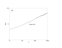
Figure 1: Only the local mutation rule allows the number of observable species to continue to increase. (a) The horizontal axis $\tau$ represents the time measured with respect to the interval between ‘mutations’. The vertical axis represents the number of observable species $\bar{S}(\tau)$. (b) The log-log plot of $\bar{S}(\tau)$ under the local rule from (a) and the function with which it is fitted, $\tau^{0.38}$ (dashed curve). The parameters used here are $\delta=\exp(-11)$, $\zeta=\exp(-10)$, $\xi=\exp(-9)$, $v=1.0$ and $T=900$.

As we discussed above, we consider three different rules for the variations of the interactions $\{a_{ki}\}$ and $\{a_{ik}\}$ for the new species: invasive, global and local. In the case of the invasive rule, we add a new species whose interaction coefficients are assigned randomly and are independent of all existing species (including its parent). In the case of the global rule, we produce a mutant whose interaction coefficients are all only slightly different from those of its parent species. In the case of the local rule, we introduce a mutant that is identical to its parent species, apart from its interaction with one particular surviving species. While the invasive (Robinson & Valentine, 1979; Yodzis, 1988; Happel & Stadler, 1998) and global (Ginzburg et al., 1988; Happel & Stadler, 1998; Drossel et al., 2001) rules have been employed in previous studies, the local rule is examined for the first time in the present study. In terms of theoretical population genetics, the invasive rule corresponds to the “house-of-cards” approximation (Turelli, 1983). The details of these rules are as follows.

• Invasive: We assign the values of $\{a_{ki}\}$ and $\{a_{ik}\}$ for all $i\,(\neq k)$ as Gaussian random numbers (mean 0 and variance 1). This implies that the mutant species is independent of its parent species.

• global: Quantities $\{\upsilon_{ki}\}$ and $\{\upsilon_{ik}\}$ representing Gaussian random noise with mean $0$ and variance $1$ are independently added to $\{a_{ki}\}$ and $\{a_{ik}\}$ for all $i$ according to

  $$\left(\begin{array}[]{c}a_{ki}\Leftarrow\gamma a_{ki}+(1-\gamma)\upsilon_{ki}\\ a_{ik}\Leftarrow\gamma a_{ik}+(1-\gamma)\upsilon_{ik}\end{array}\right.$$ (3)

  for all $i$, where $\gamma$ ($0<\gamma<1$) denotes the strength of the noise. In our simulations, this value was set to $0.9$.

• local: We select a species $l$ whose population is non-zero and change only the relationship between the mutant species and species $l\,(\neq k)$. Thus, the effects of a mutation are concentrated on only two elements, $a_{kl}$ and $a_{lk}$. We assigned the values of these two elements using Gaussian random numbers with mean $0$ and variance $1$.

In all cases, the intraspecies interaction $a_{ii}$ takes the value $-v$ for each species $i$. Finally, we introduce a threshold $\xi$ ($\xi>\zeta>\delta$), and we consider a species to be unobservable if its population $x_{i}$ is smaller than $\xi$. Since $\xi$ is larger than $\zeta$, a mutant species is not observable until its population increases and becomes greater than $\xi$. The function $S(\tau)$ denotes the number of the observable species existing at the end of the $\tau$th period. We regard $S(\tau)$ as the diversity in this model. It should be noted that, in general, there appear much more unobservable species than observable species although the population of the latter is much larger than that of the former.

2.2 Results

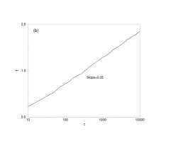
Figure 2: (a)The average fitness, $\bar{f}(t)\equiv\sum_{j,k=1}^{N(t)}a_{jk}x_{j}(t)x_{k}(t)$. All curves were obtained from an average over $50$ samples of independent simulations with different series of random numbers. (b) The log-normal plot of $\bar{f}$ under the local rule from (a) and the function with which it is fitted, $\log(\tau^{0.25})$ (dashed line).

Figure 1 (a) displays the development of $\bar{S}(\tau)$ for each of the three rules, where $\bar{S}(\tau)$ is defined as $S(\tau)$ averaged over independent simulations with different series of random numbers. We set the initial conditions as $x_{1}=1$ [that is, $N(0)=S(0)=1$] and $a_{11}=-v$. This figure shows that diversity grows most under local rule. The diversity $\bar{S}(\tau)$ under the local rule increases to approximately $50$ at $\tau=10,000$, and as can be inferred from this plot, it continues to increase beyond this value as more mutants are added. We averaged the diversity over $50$ simulations and found that this averaged value obeys $\bar{S}(\tau)\sim\tau^{0.38}$ [Figure 1(b)], which should be compared with the square root law $S(\tau)\sim\sqrt{\tau}$ in the coinfection model (May & Nowak, 1995).

Figure 2 (a) displays the development of the average fitness under the three rules. As in the case of the diversity, it is seen here that only the local rule allows for the average fitness to continue to increase. Since the average fitness $\bar{f}=\sum_{j,k=1}^{N(\tau)}a_{jk}x_{j}(\tau)x_{k}(\tau)$ is a kind of average of the interaction coefficients, we can regard this quantity as an index of mutualism. The results here therefore indicate that the diversity and the level of the mutualism increase together. It is interesting that the average fitness does not display power-law behavior, but rather increases much more slowly: $\bar{f}\sim c\log(\tau)\,(c\sim 0.25)$ (Figure 2(b)). This is analogous to the slow increase of the diversity observed in a GLVE model of super-infection in a host-parasite system (May & Nowak, 1994).

Figure 3(a) plots the development of $S(\tau)$, where the largest number of species observed for this case is $196$ at $\tau=144,700$. In the plots of Figures 3 (a) and (b), only one sample for the development of each $S(\tau)$ and $\bar{f}$ is used. By contrast, the plots in Figure 1 represent averages over $50$ samples. From Figure 3(a), we wee that the diversity does not increase monotonically, and repeated avalanches of extinction followed by rapid recoveries are observed. Figure 3(b) gives an enlarged view of the time evolution plotted in Figure 3(a) from $\tau=7,500$ to $7,900$ in order to clarify the relationship between $S(\tau)$ and $\bar{f}$. Here we observe a clear negative correlation; that is, the average fitness drastically increases during an avalanche of extinction. This behavior is typically observed in extinction dynamics (Tokita & Yasutomi, 1999). However, the average fitness does not increase during the time that the diversity increases. This implies that extinction plays a more important role than speciation in the increase of the average fitness. This is because large extinction events swiftly exterminate less mutualistic species and produce a more mutualistic network of species. The refined network then prepares for a rapid recovery of the diversity in the aftermath of the extinction.

Figure 3: (a) Development of the diversity $S(\tau)$ and the average fitness $\bar{f}$. This figure shows the result for a single sample under the local rule. (b) An enlarged view of (a) for $\tau=7500-7900$. Here $\delta=\exp(-11)$, $\zeta=\exp(-10)$, $\xi=\exp(-9)$, $v=1.0$ and $T=900$.

In the case that $S(\tau)$ is defined with just one sample, its fluctuation suggests simultaneous occurence of extinction and speciation of multiple species. On the other hand, $\bar{f}(\tau)$ develops relatively smoothly, because the definition of $\bar{f}$ is a kind of average of the interactions $\{a_{ij}\}$ over $\{x_{i}\}$, and $x_{i}$ at the time that the $i$th species appears or extincts is very small ($\delta$ for extinction and $\zeta$ for speciation).

Figure 4 plots the dependence of $\bar{S}$ on the ratio of the value of the diagonal elements, $v$, and the variance of the Gaussian random numbers ($=1$) that are used to assign the interaction coefficients of the mutant in the case of the local rule. We see that $\bar{S}$ depends only weakly on $v$. We should note that May (1972) showed that the internal equilibrium point becomes unstable when this value becomes less than $1$ if the system is assembled randomly at one time, rather than through the periodic introduction of mutants, as done in our study. The strength of the interactions between species affects the stability of the ecosystem if it is assembled at one time, but it does not do so when the ecosystem gradually develops for a long time on the evolutionary time scale.

Figure 4: The observable diversity $\bar{S}(\tau)$ at $\tau=10,000$ displayed as a function of $v$ under the local rule. $v$ represents the value of diagonal elements of the interaction matrix (the intraspecies interaction), while the off-diagonal interspecies interactions are assigned as Gaussian random numbers with mean $0$ and variance $1$. Here $\delta=\exp(-11)$, $\zeta=\exp(-10)$, $\xi=\exp(-9)$ and $T=100$. Each dot corresponds to an average over 10 samples of independent simulations.

Why does the diversity $S(\tau)$ increase so drastically only in the case of the local rule? To answer this question, let us consider Figure 6, which gives an example of our numerical integration. This figure shows that a few species enter the existing ecosystem more rapidly than exponentially and virtually simultaneously. This kind of rapid population growth results from the fact that the relationship between these mutant species is more mutualistic than those between the dominant species. When the relationship between mutants $p$ and $q$ is more mutualistic than those between the dominant species, and this relationship therefore makes these mutants “fitter” than the average species, their population increase. The growth of the population of species $p$ thus increases the fitness of species $q$, thereby enhancing its growth rate, and hence increasing the fitness of $p$. These unobservable species constitute a new mutualistic unobservable subsystem and eventually merge into the observable existing ecosystem. The implication of this behavior is that the formation of a mutualistic network is more effective as a invasion strategy than competition or even exploitation under the pressure of natural selection, because a mutualistic invasion has the abovementioned positive feedback effect, while the exploitation involves a negative feedback (as the more one species preys on another, the less abundant this prey becomes).

Figure 5: A few mutant species grow more rapidly than exponentially, and they enter into the observable ecosystem at virtually the same time. Here $\delta=\exp(-11)$, $\zeta=\exp(-10)$, $\xi=\exp(-9)$, $v=1.0$ and $T=900$.

Figure 6: Mutant species produced through the mutational rule grow less rapidly than exponentially. After entering the ecosystem, they usually come to replace their parent species. Here $\delta=\exp(-11)$, $\zeta=\exp(-10)$, $\xi=\exp(-9)$, $v=1.0$ and $T=900$.

In order to form such a subsystem, mutants must wait for the arrival of partners. In order to avoid extinction while waiting, such a mutant must have virtually the same fitness as its parent species. More precisely, they must have the same interaction coefficients with respect to the dominant species as their parents. If this is not the case, they will independently invade the existing ecosystem, replacing their parent species, or they will simply be repulsed. Of course, the invasive and global rules rarely produce such “sleeping” mutants, because in general in these cases all interactions of a given mutant will be different from those of their parents. Figure 6 gives an example of our numerical integration for the case of the global rule. Here a new species invades independently, replacing an existing species, and we can observe no faster-than-exponential population growth. Only the local rule can produce such mutants, and this is the reason why only it can yield a remarkable increase in the diversity.

Since a subsystem of the type described above has a higher degree of mutualism than the observable system, we expect that the ecosystem will become more mutualistic as the diversity increases. Since the average fitness $\bar{f}=\sum_{j,k=1}^{N(t)}a_{jk}x_{j}(t)x_{k}(t)$ is a kind of average of the interaction coefficients, we can regard this average as an index of mutualism. As seen in Figure 1, it continues to increase only under the local rule. Figure 8 exhibits the distribution of $\{a_{ij}\}$ for an ecosystem that has emerged under the local rule. It should be noted that these values are ‘naturally selected’ from Gaussian random numbers with mean $0$ and variance $1$. As seen in the figure, the average of the distribution shifts to the positive area. This suggests that the relationships between species tend to become more and more mutualistic through the struggle for survival.

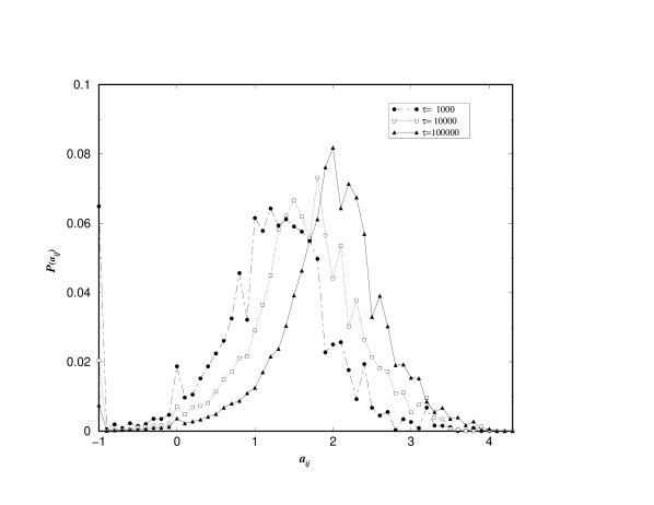
Figure 7: The vertical axis represents the frequency, and the horizontal axis represents the values of the off-diagonal elements of the matrix $(a_{ij})$ produced under the local rule. The distribution of the elements of this interaction matrix shifts toward the positive direction as time increases. The distribution is averaged over 10 samples of simulations. Here $\delta=\exp(-11)$, $\zeta=\exp(-10)$, $\xi=\exp(-9)$, $v=1.0$ and $T=900$.

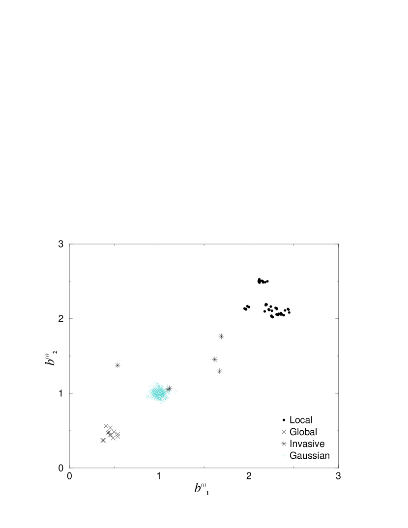
Figure 8: The distributions of the ${\vec{b}^{(i)}}$ for each species under invasive, global and local rules at $\tau=10,000$. For reference, the ${\vec{r}^{(i)}}$ (described in the main text) also appear. As seen here, the ${\vec{b}^{(i)}}$ under the local rule deviate greatly from the ${\vec{r}^{(i)}}$. Here $\delta=\exp(-11)$, $\zeta=\exp(-10)$, $\xi=\exp(-9)$, $v=1.0$ and $T=900$.

Let us consider in detail the process of speciation by introducing a $2S(\tau)$-dimensional trait space, where each species $i$ is characterized by the point $(a_{i1},a_{i2},\ldots,a_{i,S(\tau)},a_{1i},a_{2i},\ldots,a_{S(\tau),i})$. In order to visualize the distribution of the species in this high-dimensional space, we project this point onto a point in a two-dimensional space:

$${\vec{b}^{(i)}}=({b^{(i)}_{1}},{b^{(i)}_{2}})\equiv\frac{1}{S(\tau)}\left(\sqrt{\sum_{k}a_{ki}^{2}}_{,}\quad\sqrt{\sum_{j}a_{ij}^{2}}\right)_{.}$$ (4)

If the ecological status of two species $k$ and $l$ are similar, ${\vec{b}^{(k)}}$ and ${\vec{b}^{(l)}}$ are close to each other.

Figure 8 displays the sets $\{{\vec{b}^{(i)}}\}$ for each species with the interaction matrices resulting from invasive, global and local rules. For the sake of contrast, we also display the points ${\vec{r}^{(i)}}$, defined in the same way as the ${\vec{b}^{(i)}}$, for a $50\times 50$ matrix whose off-diagonal elements are given as Gaussian random numbers with mean $0$ and variance $1$. We can see that the sets $\{{\vec{b}^{(i)}}\}$ for these three interaction matrices differ greatly from $\{{\vec{r}^{(i)}}\}$. This suggests that it is quite inappropriate to use a random matrix to approximate an interaction matrix of a real ecosystem. Among these three sets $\{{\vec{b}^{(i)}}\}$, that obtained from the local rule in particular is shifted in relation to $\{{\vec{r}^{(i)}}\}$ more mutualistic region in the trait space. This is suggested also by Figure 8. Moreover, several groups of species are observed in this case, indicating that the speciation processes under the local rule do not result in a simple random drift or a random diffusion in the trait space; that is, the groups of species that appear in this case are fixed by the pressure of natural selection.

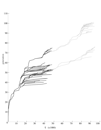
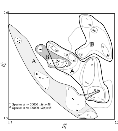
Figure 9: (a): The genealogy of surviving species at $\tau=50,000$ and $100,000$. Each species is plotted as a point whose location is determined by the time that this species emerged (horizontal axis) and the generation that this species represents (vertical line). Mother species and their daughter species are connected by lines. The connections between existing species at $\tau=50,000$ and their ancestors appear as black lines, and those at $\tau=100,000$ as gray lines. (b): This figure shows the following; (1) species closely related in lineage possess similar characteristics (at least to the extent that these are captured by the quantity plotted here); (2) there is a hierarchical structure reminiscent of a family-genus-species; and (3) almost all species existing at $\tau=50,000$ are extinct at $\tau=100,000$, and the descendants of only three species survive and produce a large number of descendents (adaptive radiation). Black circles indicate $\{{\vec{b}^{(i)}}\}$ at $\tau=50,000$ and white circles at $\tau=100,000$. Here $\delta=\exp(-11)$, $\zeta=\exp(-10)$, $\xi=\exp(-9)$, $v=1.0$ and $T=900$. Species which belong to a given branch are enclosed within the same closed curve. The thin closed curves correspond to new branches, and the thick closed curves correspond to old branches. Thus the thin curves enclose a single genus and the thick curves enclose a family.

Figure 9 displays the relationship between species in the case of the local rule. It is observed that this ecosystem starts from a single species, and the diversity increases through speciation. Figure 9(a) displays the history of the speciation. The black lines indicate a genealogy of species existing at $\tau=50,000$, and the gray lines at $\tau=100,000$ from their ancestors at $\tau=0$ and $\tau=50,000$, respectively. Lines representing the extinct species before $\tau=50,000$ and $\tau=100,000$ are not plotted, although there are in fact more branches for the extinct species. At $\tau=50,000$ there exist 58 species, and they are separated into two large groups which branches at a very early stage.

Figure 9(b) displays the points ${\vec{b}^{(i)}}$ for each species. The set $\{{\vec{b}^{(i)}}\}$ at $\tau=50,000$ is plotted with black dots and those at $\tau=100,000$ as circles. We observe two large groups in this figure: Groups A and B contain 39 and 19 species at $\tau=50,000$, respectively. Those species on the same branch of the genealogy are plotted near each other in the 2-dimensional space. We also observe several subgroups in each group: Group A contains four subgroups and group B contains two. These groups also reflect the structure of genealogy, as those species in the same subgroup appear on the same sub-branch of the genealogy. If we think of each dot and circle as a ‘species’, then each subgroup can be thought of as a ‘genus’ and an entire group is a ‘family’. The two families A and B still exist at $\tau=100,000$, shifting toward the upper right. All species at $\tau=50,000$ are extinct, and those descendants of only three species survive at $\tau=100,000$. Each arrow denotes a radiation from one of these three to a group or a subgroup at $\tau=100,000$. Descendants of one species of family A radiated into $32$ species. This family separated into two genera, and even these genera formed subsubgroups. There are $13$ species of descendants that emerged from two species of family B: one of these genera contains $4$ species and the other 9 species. The latter genus is separated into $4$ sub-genera.

Figure 10: Rank-size plot of the population densities $x_{i}$ for $178$ observable species at $\tau=150,000$.

Finally, we note the interesting correspondence of a result obtained in the present study to a well-known ecological law of population abundance: As seen from Figure 10, the dominance-diversity distribution is $S$-shaped, and its middle part displays a power law behavior. Such behavior is observed in many species-rich communities (Hubbell, 1997; Magurran, 1988). This suggests that the present model shares some characteristics with populations in nature. Let us here note that our data were not obtained through any averaging, but from only one simulation. This is significant because in order to obtain such a distribution using one sample, it is required that the sample produce a sufficiently large number of species. This has been realized for the first time in the present study.

In the present study, we have mentioned “invasion type” mutants with respect to species-specific interaction by the local rule. However we can also think of ”mutant type” mutants with respect to species-specific interaction, which have the parameter deviated from the parent’s value by a random quantity. We have executed similar simulations by such a mutative local rule and found a similar diversification like the local rule. Under the mutative local rule, the diversity $S(\tau)$ increases little slower but is fitted by a power function like under the local rule.

From the above discussion, we conclude that an ecological system which is composed of many hierarchically structured species strongly interacting with each other can emerge through an evolutionary speciation process by the local rule.

3 Resistance to Invasion

3.1 Method

As mentioned in the first section, Elton (1958) suggested that complex communities are more stable than simple ones. In this context, as pointed out by Case (1990, 1991), Elton’s definition of the ‘stability’ is not the asymptotic stability of the assembled matrix but the resistance to invasion of communities. We thus can understand his hypothesis as an assertion that species-rich ecosystems are more resistant to invasion by exotics than are species-poor ones.

Case (1990, 1991) constructed models to check Elton’s hypothesis from this point of view. He randomly assembled ecosystems and selected stable and feasible ones. Then he tested their resistance to invasion by adding new species generated by a rule very similar to our invasive rule. He concluded that a more diverse and more strongly connected ecosystem has greater resistance to invasion.

3.2 Results

We carried out a similar test on ecosystems formed under the global and local rules and compared the resistance to invasion of these ecosystems. There is an important difference between these two rules and the invasive rule. Under the global and local rules, new species are mutants of the existing species. However, under the invasive rule these are independent of the existing species, invading from without. In our tests, we added mutants generated by the local and global rules for only the first $R$ periods, and then we let invaders generated by the invasive rule attack the ecosystem for 200 periods. $R$ denotes a kind of maturity index of the ecosystem.

The results of our experiment are depicted in Figure 11, which shows the dependence of the resulting diversity $S(\tau)$ on $R$. As seen there, when $R$ is small, the diversity is drastically reduced under either rule. However, when $R$ is larger than $200$, ecosystems developed under the local rule maintain their diversity, resisting invasion. Contrastingly, those developed under the global rule exhibit a reduction in their diversity for any value of $R$, as a result of destructive invasions. This result suggests that an ecosystem developed under the local rule has strong resistance to invasion if it is sufficiently mature.

Figure 11: After $R$ periods of assemblage under local and global rules, invaders generated by the invasive rule attack for 200 periods. When $R$ is small, the invaders succeed in destroying the existing ecosystem. However, When $R$ is larger than 100, the ecosystem developed under local rule can maintain its diversity. Contrastingly, that developed under the global rule experiences a reduction in diversity resulting from attacks by invaders. Here $\delta=\exp(-11)$, $\zeta=\exp(-10)$, $\xi=\exp(-9)$, $v=1.0$ and $T=900$.

The difference between the local and global rules results from the difference in their levels of mutualisms. As we have seen in the previous section, an ecosystem evolving under the local rule is more mutualistic than one evolving under the global rule. We should note that the average fitness $\bar{f}$ here again turns out to play an important role as an index indicating the resistance to invasion . If an ecosystem has an average fitness $\bar{f}$, the fitness $f_{I}$ of an invader must be larger than $\bar{f}$ in order for the invader to succeed. Since $f_{I}$ can be approximated by a Gaussian random number with mean $0$ and variance $1$, for an ecosystem with sufficiently large diversity, the probability for a successful invasion is given by the error function,

$${\rm Prob.}(f_{I}>\bar{f})={\rm Erfc}(\bar{f})=\frac{1}{\sqrt{2\pi}}\int_{\bar{f}}^{\infty}{\rm exp}\left(-\frac{t^{2}}{2}\right){\rm d}t,$$ (5)

which decreases exponentially as $\bar{f}$ increases. From Figure 1(b), it is possible to estimate the probability (5) by using the value of $\bar{f}$ for $R\sim 200$ at which the difference between the local and global becomes larger in Figure 11. The average fitness for the local rule, $\bar{f}(\tau=200)\sim 1$, gives ${\rm Erfc}(1)\sim 0.16$, while that for the global rule, $\bar{f}(\tau=200)\sim 0.25$, gives ${\rm Erfc}(0.25)\sim 0.4$. Figure 1(b) indicates that $\bar{f}$ is a monotonically increasing function of $R$ for the local rule, and hence we expect that a random invasion becomes almost impossible against a fully-matured ecosystem (i.e., one of large $R$) under the local rule. That is, only temporally neutral mutants can influence or create extinction events in an existing ecosystem evolved under the local rule.

4 Discussion

Generalized Lotka-Volterra equations vs. replicator equations

The generalized Lotka-Volterra equations (GLVE) are more commonly used than the replicator equations (RE) in the field of mathematical biology. However, it is known that an $N$-dimensional RE is mathematically identical to the ($N-1$)-dimensional GLVE (Hofbauer & Sigmund, 1998)

$$\frac{{\rm d}y_{i}}{{\rm d}t}=y_{i}(r_{i}+\sum_{j=1}^{N-1}b_{ij}y_{j})\qquad(i=1,2,\cdots,N-1),$$ (6)

where the $i$th species’ population $y_{i}$ is defined in terms of the population in the RE (1), $x_{i}$ by

$$y_{i}=\frac{x_{i}}{x_{N}}.$$ (7)

The value of $y_{i}$ can take any non-negative real number. The interactions $\{b_{ij}\}$ and the intrinsic growth (or decay) rate $r_{i}$ here are defined in terms of interactions in the RE by

$$b_{ij} = \left.a_{ij}-a_{Nj}\right._{,}$$ (8)

$$r_{i} = \left.a_{iN}-a_{NN}=a_{iN}+v\right._{.}$$ (9)

Any orbit of the GLVE can therefore be mapped onto an equivalent orbit of the RE, and any behavior exhibited by these two systems can be studied using either, at least in principle.

Here we explain why we nevertheless study the RE rather than the GLVE. As described in the first section, Taylor (1988b) pointed out that most of the dynamics resulted in explosions of populations as proportion of species with $r_{i}>0$ increased or proportion of positive $b_{ij}$ increased. Moreover, the populations of species with low fitness often take extremely small values that cause underflow in naive numerical computational scheme. Consequently, numerical analysis of the GLVE often encounters both divergence and underflow, in particular for a system with high diversity and complex interactions. On the other hand, in the RE, population explosions are avoided by definition, because any orbit of the population $\{x_{i}\}$ is bound in the simplex $\sum_{i=1}^{N}x_{i}=1$. Moreover, in the present model, the problem of underflow is also avoided because the heteroclinic orbits, the cause of underflow, are excluded by the introduction of the extinction threshold (Tokita & Yasutomi 1999). These are the reasons we use the RE rather than the GLVE.

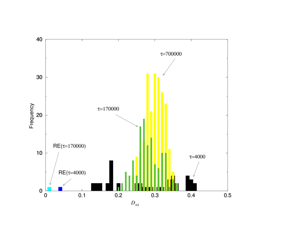
Figure 12: The vertical axis represents the frequency, and the horizontal axis represents the values of the antisymmetricity $D_{AS}(B)$ at $\tau=4,000,170,000$ and $700,000$ and $D_{AS}(A)$ at $\tau=4,000$ and $170,000$ (“RE”). The value of the antisymmetry $D_{AS}(A)$ at $\tau=700,000$ becomes nearly zero. Here $\delta=\exp(-11)$, $\zeta=\exp(-10)$, $\xi=\exp(-9)$, $v=1.0$ and $T=1,000$.

Let us note that the meaning of the interaction coefficients $a_{ij}$ in the RE is different from that of the $b_{ij}$ in the GLVE: even if the $a_{ij}$ and $a_{ji}$ take only positive values (mutualistic relationships), the $b_{ij}$ and $b_{ji}$ can take negative values (competitive or exploitative relationships) depending on the values of $a_{ij}$ and $a_{Nj}$ in Eq. (8). As the growth rate of the species $i$ is defined by the fitness $\sum_{j}a_{ij}x_{j}$ deducted by its average $\sum_{j,k}a_{jk}x_{j}x_{k}$ in the definition of the replicator equations (1), the ecological significance of the developed ecosystem in the present study should be discussed by the matrix $B=(b_{ij})$ in the GLVE than $A=(a_{ij})$ in the RE. We therefore study the nature of matrices $B$ transformed from $A$ by Eq. (8). Here we should note that there are $N$ ways of transformation from $A$ to $B$ because of the arbitrary option of the species $N$ in Eq. (7). To characterize a $L\times L$ matrix $M=\{m_{ij}\}$, here we define “antisymmetricity” as

$$D_{AS}(M)\equiv\left.\frac{\langle(m_{ij}-m_{ji})^{2}\rangle_{M}}{4\langle m_{ij}^{2}\rangle_{M}}\right._{.}$$ (10)

The bracket $\langle(\cdots)\rangle_{M}\equiv\frac{1}{L(L-1)}\sum_{i=1}^{L}\sum_{j\neq i}^{L}(\cdots)$ denotes the average over all off-diagonal elements of $M$. For the RE with interaction $A$ at $\tau$, $L$ becomes $S(\tau)$, and $L=S(\tau)-1$ for $B$ of the corresponding GLVE. In general, the antisymmetricity $D_{AS}(M)$ becomes $0$, $1/2$ and $1$ when $M$ is symmetric ($m_{ij}=m_{ji}$), randomly asymmetric ($m_{ij}\neq m_{ji}$) and antisymmetric ($m_{ij}=-m_{ji}$), respectively. Figure 12 plots the distribution of $D_{AS}(B)$ at $\tau=4,000,170,000\mbox{ and }700,000$, where $S(4,000)=45,S(170,000)=125\mbox{ and }S(700,000)=216$. The value of the antisymmetry $D_{AS}(A)$ of the RE at $\tau=4,000,170,000$ is also indicated. From the figure, the interaction matrix $A$ of the RE turns out to approach the symmetric point ($D_{AS}=0$; mutualism). On the other hand, the matrix $B$ tends to approach the intermediate region ($D_{AS}\sim 0.3$) between symmetric and asymmetric. This implies that the system evolved under the local rule has complex ecological interspecies interactions including mutualism, competition, predation and parasitism.

From the figure 8 and 12, we conclude that the frequency of the interspecies interactions of the emerged system can be approximated by a symmetric Gauss distribution with mean $m(>0)$ and variance $1$

$$P(a_{ij}) = \frac{1}{\sqrt{2}}\exp\left(-\frac{(a_{ij}-m)^{2}}{2}\right),\quad(\mbox{for}\quad i\neq j\quad\mbox{and}\quad a_{ij}=a_{ji})$$ (11)

$$a_{ii} = -v(<0)$$ (12)

in the infinite limit of the number of species ($N\to\infty$), where $m>0$ is the level of mutualism. This type of the replicator equation, in general, has a number of saturated fixed points, which is proved by the symmetry of the interaction (Hofbauer & Sigmund, 1998).

Finally, let us see how {$r_{i}$} and {$b_{ij}$} in the corresponding GLVE mutate in the local rule. First, values $r_{k}$, {$b_{ik}$} and {$b_{ki}$} for all $i$ of a new species $k$ are copied from $r_{j}$, {$b_{ij}$} and {$b_{ji}$} of a parent species $j$, respectively. Second, by the definition of the local rule and the transformation (8) and (9), $r_{k}$ or $b_{lk}$ (and $b_{kl}$) for arbitrary $l$ is replaced by a random quantity. Note that $r_{k}$ is replaced by a random number with mean $v$ and variance $1$ while $b_{lk}$ ($b_{kl}$) with mean $0$ and variance $1$. From the transformation (8) and the distribution (11) and (12) of $a_{ij}$, the distribution of $b_{ij}$ becomes a Gauss distribution with mean $0$ and, therefore, is not mutualistic. Minor mutualist species in the RE, therefore, are not necessarily mutualists in the GLVE, and do not necessarily lead population explosion. On the other hand, $r_{i}$ in Eq. (9) is biased by $v(>0)$ and the mean value of $r_{i}$ increases over time because mean value of $a_{iN}$ increases as indicated by Fig. 8. Accordingly, in terms of the GLVE, proportion of producers increases as time goes on in the local rule. As pointed out by Taylor (1988b), this may trigger population explosion. Another chance for explosion is implied in the transformation (7) when the $N$-th “base” species goes extinct ($x_{N}(t)\to 0$), which breaks down the simulation of the corresponding GLVE. We stress here that even if the extinction of one “base” species causes the explosion in the GLVE, the evolution in the RE proceeds successfully and there are still other equivalent GLVE systems by transformations by other $N-1$ “base” species as $y_{i}=x_{i}/x_{M}$ ($M=1,2,\cdots,N-1$). The RE, therefore, traces a possible path of evolution avoiding the breakdown of the simulation which may occur in the GLVE. This methodological advantage of the RE is related to the circumstance that the dimension (the degree of freedom) of the RE is one higher than the GLVE and the total population is conserved (Eq. (2)). This suggests that such a conservative quantity, e.g. resource limitations, would be essential in the modeling of multispecies evolution using the GLVE.

The authors would like to thank Yoh Iwasa, Takashi Ikegami and Tsuyoshi Chawanya for their helpful comments on the manuscript and for their encouragement. This work was partially supported by the Japan Society for the Promotion of Science, a Grant-in-Aid from the Ministry of Education, Science, Sports and Culture of Japan (No. 12740235, 13831007 and 14740232), and the Suntory Foundation. Some of the numerical calculations were carried out on a Fujitsu VPP500/40 at the Supercomputer Center, Institute for Solid State Physics, University of Tokyo and on the Machikaneyama PC Cluster System in the Condensed Matter Theory Group, Graduate School of Science, Osaka University (URL: http://wwwacty.phys.sci.osaka-u.ac.jp/~mhill).

References

- [1] Brown, J. S. and Vincent, T. L. (1992) Organization of predator-prey communities as an evolutionary game. Evolution 46, 1269-1283.
- [2] Case, T. J. (1990) Invasion resistance arises in strongly interacting species-rich model competition communities. Proc. Natl. Acad. Sci. USA, 87, 9610-9614.
- [3] Case, T. J. (1991) Invasion resistance arises in strongly interacting species-rich model competition communities. In: Metapopulation dynamics. Biological Journal of the Linnean Society, (Gilpin, M. E. & Hanski, I. eds.), 42, pp.239-266, London: Academic Press.
- [4] Chawanya, T. (1995) A new type of irregular motion in a class of game dynamics systems, Prog. Theor. Phys. 94, 163-179.
- [5] Chawanya, T. (1997) Coexistence of infinitely many attractors in a simple flow, Physica D 109, 201-241.
- [6] Chawanya, T. & Tokita, K. (2002) Large-Dimensional Replicator Equations with Antisymmetric Random Interactions, J. Phys. Soc. Japan 71, 429-431
- [7] Colwell, R. K., & Winkler, D. W. (1084) A null model for mull models in biogeography. In:Ecological Communities: Conceptual issues and the evidence, (Strog D. R., Simberloff, D., Abel, L. B., Thistle, A. B. , eds), Princeton University Press.
- [8] Drake, J. A. (1990) The mechanics of Community Assembly and Succession. J. theor. Biol., 147, 213-233.
- [9] Drossel, B. Higgs, P. G. & McKane, A. J. (2001) The Influence of Predator-Prey Population Dynamics on the Long-term Evolution of Food Web Structure. J. theor. Biol., 208, 91-107.
- [10] Elton, C. S. (1958) The ecology of invasions by animals and plants, Chapman and Hall, London.
- [11] Gardner, M. R., & Ashby, W. R. (1970) Connectance of large dynamic (cybernetic) systems: Critical values for stability. Nature 228, 784-784.
- [12] Geritz, S. A. H., Kisdi, E., Meszena, G. and Metz, J. A. J. (1998) Evolutionarily singular strategies and the adaptive growth and branching of the evolutionary tree. Evol. Ecol., 12, 35-57.
- [13] Gilpin, M. E., & Case, T. J. (1976) Multiple domains of attraction in competition communities. Nature, 261, 40-42.
- [14] Ginzburg, L. R., Akçakaya, H. R., & Kim, J. (1988) Evolution of community structure: Competition, J. theor. Biol., 133, 513-523.
- [15] Happel, R., & Stadler, P. F., (1998) The evolution of diversity in relicator networks. J. theor. Biol., 195, 329-338.
- [16] Hofbauer, J. , & Sigmund K. (1998) Evolutionary Games and Population Dynamics, Cambridge University Press.
- [17] Hubbell, S. P. (1979) Tree dispersion, abundance and diversity in a tropical dry forest. Science, 203, 1299-1309.
- [18] Hubbell, S. P. (1997) A unified theory of biogeography and relative species abundance and its application to tropical rain forests and coral reefs. Coral Reefs, 16, Suppl.:S9-S21.
- [19] Hubbell, S. P. (2001) The Unified Neutral Theory of Biodiversity and Biogeography, Princeton University Press.
- [20] Kimura, M. (1983) The neutral theory of molecular evolution, Cambridge University Press
- [21] King, A. W., & Pimm, S. L. (1983) Complexity and stability: a reconciliation of theoretical and experimental results. Am. Nat., 122, 229-239.
- [22] Law, R. & Morton, R. D. (1996) Permanence and the assembly of ecological communities, Ecology, 77, 762-775.
- [23] MacArthur, R. H. (1955) Fluctuations of animal populations and a measure of community stability, Ecology, 36, 439-454.
- [24] Magurran, A.E., (1988) Ecological diversity and its measurement, Croom Helm Ltd, London.
- [25] May, R. M. (1972) Will a large complex system be stable? Nature, 238, 413-414.
- [26] May, R. M. (1974) Stability and complexity in model ecosystems 2nd ed. Princeton University Press
- [27] May, R. M. & Leonard, W. J. (1975) Nonlinear aspects of competition between three species. SIAM J. Appl. Math. 29, 243-252
- [28] May, R. M. & Nowak, M. A. (1994) Superinfection, metapopulation dynamics, and the evolution of diversity. J. theor. Biol. 170, 95-114.
- [29] May, R. M. & Nowak, M. A. (1995) Coinfection and the evolution of parasite virulence. Proc. R. Soc. London B 261, 209-215.
- [30] Pimm, S. L. (1991) The balance of nature?, Chicago University Press.
- [31] Post, W. M. , & Pimm, S. L. (1983) Community assembly and food web stability, Math. Biosci., 64, 169-192.
- [32] Roberts, A. (1974) The stability of a feasible random ecosystem, Nature 251, 607-608.
- [33] Roberts, A. , & Tregonning, K. (1980) The robustness of natural systems, Nature, 288, 265-266.
- [34] Robinson, J. V. , & Valentine, W. D. (1979) Does invasion sequence affect community structure?, Ecology, 68, 587-595.
- [35] Sasaki, A. (1997) Clumped distribution by neighborhood competition. J. theor. Biol. 186, 415-430.
- [36] Taylor, P. T. (1988a) Consistent scaling and parameter choice for linear and generalized Lotka-Volterra models used in community ecology. J. theor. Biol., 135, 543-568.
- [37] Taylor, P. T. (1988b) The construction and turnover of complex community models having generalized Lotka-Volterra dynamics. J. theor.Biol., 135, 569-588.
- [38] Tokita, K., & Yasutomi, A. (1999) Mass Extinction in a Dynamical System of Evolution with Variable Dimension. Phys. Rev. E, 60, 682-687.
- [39] Tregonning, K. , & Roberts, A. (1979) Complex systems which evolve towards homeostasis. Nature, 281, 563-564.
- [40] Turelli, M. , (1983) Heritable genetic variation via mutation-selection balance: Lerch’s zeta meets the abdominal bristle. Theor. Pop. Biol., 25, 138-193.
- [41] Yodzis, P. (1988) The indeterminancy of ecological interactions as perceived through perturbation experiments. Ecology, 69, 508-515.