Euroattractor: a brief introduction to Iterated Function Systems

Abstract

In this work we propose a definition of an Euroattractor: an attracting invariant measure of a certain iterated functions system (IFS). An IFS is defined by specifying a set of functions, defined in subsets of ${\mathbb{R}}^{N}$ or in a classical phase space, which act randomly on the initial point, so it may be considered as a generalization of the notion of classical dynamical system. If the functions are sufficiently contracting, there exists an invariant measure of the system, often concentrated on a fractal set. We investigate invariant measures of a certain class of generalized or weakly contracting IFS’s.

I Introduction

Any function $f$ which maps a phase space $\Omega$ into itself may be considered as a classical dynamical system. An arbitrary point $x\in\Omega$ determines the trajectory uniquely, $x_{n}=f^{n}(x_{0})$, where the natural index $n$ plays the role of time. Dynamical system defined by $f$ is deterministic. There exist different ways to introduce randomness into the system. One possibility relays on taking into account an additive noise, $x_{n+1}=f(x_{n})+\xi_{n}$, where $\xi_{n}$ are uncorrelated random variables drawn according to a prescribed probability distribution $P(\xi)$. The deterministic case is obtained if $P(\xi)$ tends to the Dirac delta distribution, $P(\xi)=\delta(\xi)$.

In this work we analyze another class of stochastic systems, in which the choice of a system is random at each step. Such systems are called Iterated Function System (IFS), and may be considered as a generalization of the notion of a classical dynamical system.

An IFS is defined Ba by a set of $k$ functions $f_{i}:\Omega\to\Omega$, which represent dynamical systems in the classical phase space $\Omega$. The functions $f_{i}$ act randomly with given probabilities $p_{i}$. They characterize the likelihood of choosing a particular map at each step of the time evolution of the system. In general, the probabilities may be place dependent.

Analyzing a given iterated function system, one may ask, how an initial point $x_{0}\in\Omega$ is transformed by the random process. One may also consider a more general question, how does a probability measure $\mu$ on $\Omega$ change with respect to the Frobenius-Perron operator $M$ associated with the IFS. If the functions $f_{i}$ are strongly contracting, then there exists unique invariant measure $\mu_{*}$ of $M$ – see for instance K81 ; E87 ; Ba ; BDEG88 and references therein.

Interestingly, for a large class of IFS’s the invariant measure $\mu_{*}$ is characterized by a fractal structure. If the invariant measure is attracting, such IFS’s may be used to generate fractal sets in the space $\Omega$. In particular, there exist iterated function systems leading to popular fractal sets: Cantor set, Sierpinski carpet or Sierpinski gasket Ba . In fact by considering a slightly generalized class of IFS’s it is possible to design a random system, the invariant measure of which possesses any desired properties. In this work we shall visualize the statement, by presenting an Euroattractor - a system, the attractor of which has the shape resembling the contours of Europe.

This paper is organized as follows. In the next section we recall the definition and basic properties of the standard IFS. Section III is devoted to a weakly contracting IFS, which exhibit nontrivial invariant measures, although they do not fulfill the standard contractivity assumptions. In section IV we define a generalized class of the systems and present the definition of an Euroattractor.

II Iterated Function Systems

An iterated function system (IFS) is defined by a set of $k$ functions (dynamical systems) $f_{i}$, $i=1,...,k$, defined on a compact space $\Omega$ and the set of $k$ positive probabilities $p_{i}$, which sum to unity. In the IFS of the first kind the probabilities are constant, while in the more general, IFS of the second kind BDEG88 ; SKZ00 , they are functions of the position, $p_{i}=p_{i}(x)$. For any $x\in\Omega$ the condition $\sum_{i=1}^{k}p_{i}(x)=1$ has to be fulfilled. In general, IFS $\cal F$ is defined by a set ${\cal F}=\{\Omega,f_{i}:\Omega\to\Omega,p_{i}:\Omega\to[0,1]\}$ with $i=1,\dots,k$.

Any IFS generates a Frobenius–Perron operator $M$, which describes the time evolution of the probability densities on $\Omega$. In the simplest case, in which the space $\Omega$ is an interval in $\mathbb{R}$ and the maps $f_{i}$ are invertible, any initial probability density $\rho(x)$ is mapped into $\rho^{\prime}(x)$ by the Frobenius–Perron operator LM94

$$\rho^{\prime}(x)=M[\rho(x)]=\sum_{i=1}^{k}p_{i}\bigl{(}f_{i}^{-1}(x)\bigr{)}\rho\bigl{(}f_{i}^{-1}(x)\bigr{)}\left|\frac{df_{i}^{-1}(x)}{dx}\right|.$$ (1)

If $\rho(x)$ is a non-singular probability density, so is $\rho^{\prime}(x)$. However, in the limit $n\to\infty$ the image $M^{n}[\rho(x)]$ needs not to be a smooth probability density, so it is advantageous to work in the larger space of probability measures on $\Omega$. This space includes also also singular measures like the Dirac delta distributions and their convex combinations.

If an IFS is sufficiently contracting, i.e.

a) the functions $f_{i}$ satisfy the Lipschitz condition, $d(f_{i}(x),f_{i}(y))\leq L_{i}d(x,y)$) for any $x,y\in\Omega$. Here $d(x,y)$ denotes the distance between both points and the Lipschitz constants $L_{i}$ are assumed to be smaller than unity,

b) the probabilities $p_{i}(x)$ are continuous functions, strictly positive for any $x\in\Omega$, the IFS is called hyperbolic and there exists a unique invariant probability measure $\mu_{*}$ satisfying the equation $M\mu_{*}=\mu_{*}$ LM94 .

Interestingly, the conditions a) and b) are not necessary to assure the existence of a unique invariant probability measure. Some other less restrictive sufficient assumptions which regard also IFS of the second kind, with place dependent probabilities, were analyzed in K81 ; E87 ; BE88 ; BDEG88 ; LY94 ; JL95 ; E96 ; Sz00 .

The invariant measures of an IFS display often fractal properties. For instance, consider an IFS of the first kind defined on an interval and consisting of $k=2$ affine transformations,

$${\cal F}_{1}=\{\Omega=[0,1],\ f_{1}(x)=x/3,\ f_{2}(x)=x/3+2/3;\quad p_{1}=p_{2}=\frac{1}{2}\}.$$ (2)

Since both functions are continuous contractions with Lipschitz constants $L_{1}=L_{2}=1/3<1$, and the probabilities $p_{i}$ are constant and nonzero this IFS is hyperbolic. Thus there exists a unique, attracting invariant measure $\mu_{*}$. It is not difficult to show Ba that $\mu_{*}$ is concentrated uniformly on the Cantor set of the fractal dimension $D=\ln 2/\ln 3$.

Although $\mu_{*}$ is singular, it is possible to give a general prescription, how to compute integrals with respect to this invariant measure. This is due to the fact that the measure $\mu_{*}$ is attractive, i.e., $M^{n}{\mu}$ converges weakly to $\mu_{*}$ if $n\to\infty$. Therefore, in order to obtain the exact value of an integral $\int_{\Omega}h(x)~{}d{\mu_{*}}$ for any continuous function $h(x)$ it is sufficient to find the limit of the sequence $h_{n}:=\int_{\Omega}h(x)~{}d(M^{n}{\mu})$ for an arbitrary initial measure $\mu$. This method of computing integrals over the invariant measure $\mu_{*}$ is purely deterministic Ba ; E96 ; Sl97 ; SKZ00 . Alternatively, one may employ a random iterated algorithm by generating by the IFS a random sequence $x_{j}\in\Omega$, $j=0,\dots,n-1$ which originates from an arbitrary initial point $x_{0}$. Due to the the ergodic theorem for IFS’s K81 ; E87 ; IG90 the mean value $\frac{1}{n}[\sum_{j=0}^{n-1}h(x_{j})]$ converges in the limit $n\to\infty$ to the desired integral, $\int_{\Omega}h(x)~{}d{\mu_{*}}$, with probability one.

To show an example of an IFS of the second kind let us change probabilities in ${\cal F}_{1}$ and define

$${\cal F}_{2}=\{\Omega=[0,1],\ f_{1}(x)=x/3,\ f_{2}(x)=x/3+2/3;\quad p_{1}(x)=x,\ p_{2}(x)=1-x\}.$$ (3)

The probability $p_{2}$ vanish at the point $x=1$, so this IFS is not hyperbolic. In spite of this fact there exists the unique invariant measure $\mu_{*}$ concentrated in a non-uniform way on the Cantor set SKZ00 . In this case $\mu_{*}$ displays multifractal properties, since the generalized dimension of the measure depends on the Rényi parameter BS93 .

III Weakly contracting IFS

Contraction conditions a) and b) imply existence of a unique invariant measure for the IFS. However, these conditions are too strong, and there exist IFSs with an attracting invariant measure which do not obey them. If the space $\Omega\subset{\mathbb{R}}^{m}$ and the functions $f_{i}$ are linear, the Lipschitz condition a) is equivalent to the statement that the moduli of all elements of the Jacobi matrices $J_{i}:=\partial f_{i}(x_{1},...,x_{m})/\partial(x_{1},...,x_{m})$ are strictly smaller then one.

This is not the case for the following IFS defined on the square

$${\cal F}_{3}=\left\{\begin{array}[]{r c l}\Omega=[0,1]\times[0,1],\ k&=&2;\quad p_{1}=p_{2}=1/2\\ f_{1}(x,y)&=&(xy,~{}y)\\ f_{2}(x,y)&=&((x-1)y+1,~{}y+\delta)\end{array}\right\},$$ (4)

since the Jacobi matrices

$$J_{1}=\left(\begin{array}[c]{cc}y&x\\ 0&1\end{array}\right){\rm\quad and\quad}J_{2}=\left(\begin{array}[c]{cc}y&x-1\\ 0&1\end{array}\right)$$ (5)

contain entries equal to unity. This reflects the fact that both functions $f_{1}$ and $f_{2}$ are not contracting in the $y$–direction. Numerical experiments suggest that in spite of this fact for irrational values of $\delta\ll 1$, the associated Frobenius–Perron operator $M$ possess a unique invariant measure $\mu_{*}$. Such an IFS, not fulfilling the condition a) or b) will be called weakly contracting.

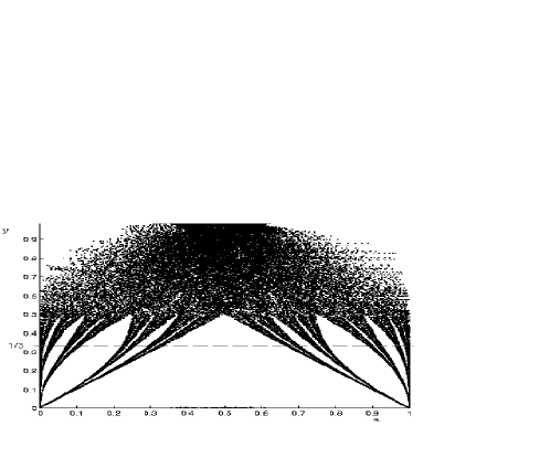
Figure 1: Invariant density of the weakly contracting IFS ${\cal F}_{3}$ (4) obtained for $\delta=\sqrt{5}/1000$. The cross-section of its support at $y=1/3$, denoted by a dashed line, forms the Cantor set.

Each random trajectory of the IFS ${\cal F}_{3}$ exhibits a slow diffusion in the $y$–direction, the speed of which is governed by the rotation parameter $\delta$. Due to periodic boundary conditions, $(x,y)=(x|_{{\rm mod}1},y|_{{\rm mod}1})$, every trajectory is confined to the square $\Omega$. If the parameter $\delta$ is chosen to be irrational, there are no periodic trajectories. If $\delta$ is sufficiently small than the contraction in the $x$–direction will dominate the diffusion in $y$, so the trajectory will be sticked to the support of the invariant measure $\mu_{*}$. Figure 1 shows a typical trajectory consisting of $6000$ points generated by this IFS. To present the asymptotic properties of the invariant measure the first $100$ points were omitted.

Note that if the parameter $\delta$ is set to zero, the variable $y$ would be fixed to the initial value $y_{0}$. Such an IFS would have an invariant measure concentrated on the interval $y=y_{0}$. Analyzing the contraction constant we see that for $y_{0}=1/3$ its support is equal to the Cantor set generated by the Cantor IFS (2). In general, for any $y_{0}<1/2$ its dimension would be

$$D(y_{0})=-\frac{\ln 2}{\ln y_{0}}\;.$$ (6)

We conjecture that this formula gives also the fractal dimension of the horizontal cross-section at $y=y_{0}$ of the invariant set of the IFS (4) in the limit $\delta\to 0$.

Another example of an invariant measure of a nonlinear, weakly contracting IFS is presented in Fig.2. The system is defined by

$${\cal F}_{4}=\left\{\begin{array}[]{r c l}\Omega=[0,1]\times[0,1],\ k&=&2;\quad p_{1}=p_{2}=1/2\\ f_{1}(x,y)&=&(\frac{1}{2}x\sin^{2}(\pi y),~{}y)\\ f_{2}(x,y)&=&(\frac{1}{2}(x-1)\sin^{2}(\pi y)+1,~{}y+\delta)\end{array}\right\}.$$ (7)

As in the previous example each random realization of the IFS generates a trajectory confined in the torus, and for small values of the shift parameter $\delta$ the contraction in the horizontal direction dominates the vertical diffusion. For $\delta=0$ the IFS reduces to one-dimensional, and the fractal dimension of its invariant set reads

$$D(y_{0})=\frac{\ln 2}{\ln 2-2\ln\sin(\pi/y_{0})}.$$ (8)

This number is smaller than one for all initial values apart of $y_{0}=1/2$. Numerical results performed for $\delta\ll 1$ suggest that the same formula describes the dimension of the cross-section at $y=y_{0}$ of the invariant set of the IFS (7) in the limit $\delta\rightarrow 0$. In other words, the support of the invariant measure $\mu_{*}$ of the IFS ${\cal F}_{4}$ may be considered as a collection of Cantor sets, with a continuously varying dimension $D(y_{0})$, placed horizontally, one parallel to another.

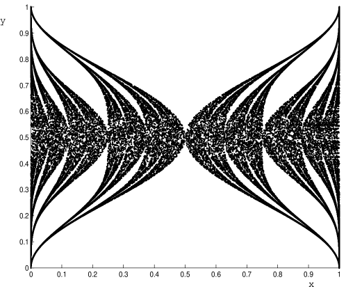
Figure 2: Invariant density of the weakly contracting IFS (7) obtained for $\delta=\sqrt{5}/1000$.

IV Repellers and generalized IFS

In the original definition of the IFS, presented in section II, all functions $f_{i}$ map the space $\Omega$ into itself. One may, however, relax this condition, and consider generalized IFS constructed of functions which map some fragments of $\Omega$ out of this space. Such functions are called repellers, since they do not conserve the probability, and during the time evolution the probability flux leaks out of the system.

A simple $1$-D repeller is obtained from the standard logistic map, $f(x)=rx(1-x)$, if the control parameter $r$ exceeds the critical value, $r_{c}=4$ Ra89 . In such systems a randomly selected initial value leads to a trajectory, which escapes the system with probability one. The complementary set of initial points which generate infinite trajectories is of measure zero and often forms a fractal set. The same property is characteristic to a large class of chaotic 1-D maps with a gap - a subset of $\Omega$ mapped out of $\Omega$. An analysis of the fractal dimension of the invariant set for the tent map with a gap is presented in ZB99 .

In this chapter we will consider an IFS defined on the square, $\Omega=[0,1]\times[0,1]$, consisting of $k$ repelling functions. Assume that each function $f_{i}$ restricted to a given set $X_{i}\subset\Omega$ acts as an affine transformation defined by real matrices $J_{i}$ of size $2$ and two components translation vectors ${\vec{\kappa}}_{i}$, but the complementary subset $\Omega\setminus X_{i}$ is mapped out of $\Omega$,

$$f_{i}\left(\begin{array}[]{c}x\\ y\end{array}\right)=\left\{\begin{array}[]{c}J_{i}\left(\begin{array}[]{c}x\\ y\end{array}\right)+{\vec{\kappa}_{i}}{\rm\quad for\quad}x\in X_{i}\\ {\rm\quad out\quad of\quad}\Omega{\rm\quad for\quad}x\notin X_{i}\end{array}\right.$$ (9)

Such functions $f_{i}$ are repelling, so instead of analyzing single trajectories, generated by a random initial point, it is convenient to work with initially smooth probability measures. Let us take for the initial measure $\mu_{0}$ the uniform (Lebesgue) measure on $\Omega$. To iterate the repelling IFS we find the images of the measures covering each of the subsets $X_{i}$ by the maps $f_{i}$, $i=1,...,k$ and add all contributions with prescribed weights – probabilities $p_{i}$. More formally, we use the the dimensional analogue of the Frobenius-Perron operator (1)

$$\rho^{\prime}(x,y)=M[\rho(x,y)]=\sum_{i=1}^{k}p_{i}\bigl{(}f_{i}^{-1}(x,y)\bigr{)}\rho\bigl{(}f_{i}^{-1}(x,y)\bigr{)}\left|\frac{\partial f_{i}(x,y)}{\partial(x,y)}\right|^{-1},$$ (10)

where the contributions from the function $f_{i}$ have to be taken into account only if the analyzed point $(x,y)$ belongs to $f_{i}(X_{i})$. Then the preimage $f_{i}^{-1}(x,y)$ exists, so the $i$-th term in the expression (10) is meaningful.

Figure 3: Generalized IFS with ’repelling’ functions $f_{i}$ which send the polygons $X_{i}$ into $X_{i}^{\prime}$, and the remaining set $\Omega\setminus X_{i}$ is mapped out of the system.

As an example of such a generalized, repelling system we consider the IFS ${\cal F}_{5}$ consisting of $k=13$ functions with equal weights, $p_{i}=1/13$. The detailed form of the affine functions $f_{i}$ as well as the definitions of the sets $X_{i}$ are provided in the Appendix. Figure 4 shows time evolution of the initially uniform measure $\mu_{0}$. The right hand side of the figure shows the measures $\mu_{n}=M^{n}[\mu_{0}]$, while the left hand side shows the sets, where the measure $\mu_{n}$ is concentrated. Initially uniform measure $\mu_{0}$ converges fast to the asymptotic measure $\mu_{*}$, and already after $n=6$ iterations can hardly be distinguished from it. The shape of the support of $\mu_{*}$ explains why the name Euroattractor has been concocted for this system.

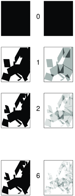
Figure 4: Euroattractor: the time evolution of the support (left) and the measure (right) of the initially uniform measure $\mu_{0}$ in the square. Already after $n=6$ iterations the measure cannot be distinguished from the invariant measure $\mu_{*}$.

V Closing Remarks

The purpose of this work was to demonstrate usefulness of the concept of Iterated Function System. This generalization of the concept of a dynamical system incorporates deterministic and stochastic behavior and may be applied in various fields of physics, and in general, of nonlinear science. A possible extension of the concept of IFS for quantum mechanics was recently worked out in LZS02 .

The IFS’s belong to a larger class of random systems studied in YOC91 ; PSV95 . From a mathematical point of view several questions concerning the rigorous theory of IFS remain open. For instance, the sufficient conditions, under which an IFS possesses a unique, attracting invariant measure are known, but the formulation of the necessary conditions remains still an exciting mathematical challenge LY94 ; G92 ; GB95 ; E96 . In this work we have introduced a weakly contracting IFS’s ${\cal F}_{3}$ and ${\cal F}_{4}$, which do not satisfy the standard contractivity conditions, but do posses attracting invariant measures.

For any given set $S$ in the plane one may try to find an IFS, such that its invariant measure $\mu_{*}$ has support on $S$. This versatility of IFS’s allows one to apply them for image synthesis, image processing and image encoding Ba ; BE88 . For instance, the attractor of a generalized IFS ${\cal F}_{5}$, described in this work, has the shape resembling the contours of Europe.

It is a pleasure to thank Radosława Bach and Wojciech Słomczyński for constructive remarks and fruitful interaction. This paper was presented at the European Interdisciplinary School on Nonlinear Dynamics Euroattractor 2002 organized in Warsaw in June 2002. We are grateful to Włodzimierz Klonowski for an inspiring name of the conference as well as for the opportunity to present this work during that event.

Appendix A An Euroattractor

In this appendix we provide an explicit definition of an Euroattractor – a generalized, repelling IFS ${\cal F}_{5}$, the invariant measure of which is shown in Fig.4. The space $\Omega$ is equal to an rectangle. To address each pixel in a simple way its size is taken to be $500\times 600$.

The IFS consists of $k=13$ affine functions $f_{i}$ defined in (9), and all the weights are constant, $p_{i}(x,y)=1/13$. The parameters defining the corners of the quadrangles $X_{i}$, and the elements of the transformation matrices $J_{i}$ and the translation vectors ${\vec{\kappa}_{i}}$ are collected in Table 1. Observe that some entries of the Jacobi matrix $J_{6}$ have modulus larger than one, so this IFS does not satisfy the contractivity condition.

Table 1. Parameters defining an Euroattractor – the IFS ${\cal F}_{5}$.

$i$	$X_{i}$	$J_{i}$	${\vec{\kappa}_{i}}$
1	$\left(\begin{array}[]{c}90\\ 370\end{array}\right)\left(\begin{array}[]{c}170\\ 520\end{array}\right)\left(\begin{array}[]{c}220\\ 350\end{array}\right)\left(\begin{array}[]{c}300\\ 500\end{array}\right)$	$\left(\begin{array}[]{cc}0.37&0.66\\ -0.74&0.66\end{array}\right)$	$\left(\begin{array}[]{c}-276\\ 371\end{array}\right)$
2	$\left(\begin{array}[]{c}520\\ 430\end{array}\right)\left(\begin{array}[]{c}340\\ 320\end{array}\right)\left(\begin{array}[]{c}420\\ 530\end{array}\right)\left(\begin{array}[]{c}240\\ 420\end{array}\right)$	$\left(\begin{array}[]{cc}-0.33&-0.73\\ 0.80&-0.59\end{array}\right)$	$\left(\begin{array}[]{c}626\\ 355\end{array}\right)$
3	$\left(\begin{array}[]{c}170\\ 350\end{array}\right)\left(\begin{array}[]{c}265\\ 480\end{array}\right)\left(\begin{array}[]{c}230\\ 320\end{array}\right)\left(\begin{array}[]{c}325\\ 450\end{array}\right)$	$\left(\begin{array}[]{cc}0.52&0.38\\ 0.01&0.68\end{array}\right)$	$\left(\begin{array}[]{c}16\\ 218\end{array}\right)$
4	$\left(\begin{array}[]{c}340\\ 300\end{array}\right)\left(\begin{array}[]{c}240\\ 420\end{array}\right)\left(\begin{array}[]{c}500\\ 400\end{array}\right)\left(\begin{array}[]{c}400\\ 520\end{array}\right)$	$\left(\begin{array}[]{cc}-0.34&0.54\\ -0.61&-0.51\end{array}\right)$	$\left(\begin{array}[]{c}192\\ 814\end{array}\right)$
5	$\left(\begin{array}[]{c}380\\ 500\end{array}\right)\left(\begin{array}[]{c}500\\ 300\end{array}\right)\left(\begin{array}[]{c}250\\ 450\end{array}\right)\left(\begin{array}[]{c}370\\ 250\end{array}\right)$	$\left(\begin{array}[]{cc}-0.17&-0.95\\ 0.96&0.08\end{array}\right)$	$\left(\begin{array}[]{c}812\\ 31\end{array}\right)$
6	$\left(\begin{array}[]{c}240\\ 460\end{array}\right)\left(\begin{array}[]{c}340\\ 550\end{array}\right)\left(\begin{array}[]{c}260\\ 440\end{array}\right)\left(\begin{array}[]{c}360\\ 530\end{array}\right)$	$\left(\begin{array}[]{cc}1.44&-1.05\\ -0.23&1.26\end{array}\right)$	$\left(\begin{array}[]{c}497\\ -24\end{array}\right)$
7	$\left(\begin{array}[]{c}200\\ 490\end{array}\right)\left(\begin{array}[]{c}50\\ 590\end{array}\right)\left(\begin{array}[]{c}150\\ 270\end{array}\right)\left(\begin{array}[]{c}0\\ 370\end{array}\right)$	$\left(\begin{array}[]{cc}-0.31&-0.47\\ -0.98&0.22\end{array}\right)$	$\left(\begin{array}[]{c}625\\ 97\end{array}\right)$
8	$\left(\begin{array}[]{c}510\\ 430\end{array}\right)\left(\begin{array}[]{c}460\\ 540\end{array}\right)\left(\begin{array}[]{c}305\\ 330\end{array}\right)\left(\begin{array}[]{c}245\\ 440\end{array}\right)$	$\left(\begin{array}[]{cc}-0.47&-0.032\\ 0.39&0.99\end{array}\right)$	$\left(\begin{array}[]{c}485\\ -438\end{array}\right)$
9	$\left(\begin{array}[]{c}230\\ 280\end{array}\right)\left(\begin{array}[]{c}230\\ 450\end{array}\right)\left(\begin{array}[]{c}460\\ 280\end{array}\right)\left(\begin{array}[]{c}460\\ 450\end{array}\right)$	$\left(\begin{array}[]{cc}0.26&1\\ -0.60&0.61\end{array}\right)$	$\left(\begin{array}[]{c}-20\\ 267\end{array}\right)$
10	$\left(\begin{array}[]{c}440\\ 280\end{array}\right)\left(\begin{array}[]{c}440\\ 450\end{array}\right)\left(\begin{array}[]{c}245\\ 280\end{array}\right)\left(\begin{array}[]{c}245\\ 450\end{array}\right)$	$\left(\begin{array}[]{cc}-0.51&0.70\\ 0.87&0.41\end{array}\right)$	$\left(\begin{array}[]{c}408\\ -339\end{array}\right)$
11	$\left(\begin{array}[]{c}250\\ 280\end{array}\right)\left(\begin{array}[]{c}310\\ 190\end{array}\right)\left(\begin{array}[]{c}220\\ 190\end{array}\right)\left(\begin{array}[]{c}270\\ 100\end{array}\right)$	$\left(\begin{array}[]{cc}-0.22&-0.37\\ 0.33&0.11\end{array}\right)$	$\left(\begin{array}[]{c}439\\ 456\end{array}\right)$
12	$\left(\begin{array}[]{c}330\\ 0\end{array}\right)\left(\begin{array}[]{c}200\\ 190\end{array}\right)\left(\begin{array}[]{c}410\\ 100\end{array}\right)\left(\begin{array}[]{c}280\\ 290\end{array}\right)$	$\left(\begin{array}[]{cc}-0.60&-0.51\\ 0.47&-0.38\end{array}\right)$	$\left(\begin{array}[]{c}359\\ 187\end{array}\right)$
13	$\left(\begin{array}[]{c}420\\ 10\end{array}\right)\left(\begin{array}[]{c}420\\ 90\end{array}\right)\left(\begin{array}[]{c}330\\ 10\end{array}\right)\left(\begin{array}[]{c}330\\ 90\end{array}\right)$	$\left(\begin{array}[]{cc}0&-0.31\\ 0.66&0\end{array}\right)$	$\left(\begin{array}[]{c}243\\ 30\end{array}\right)$

References

- (1) M. Barnsley, Fractals Everywhere, (Academic Press, San Diego, 1988).
- (2) T. Kaijser, Rev. Roum. Math. Pures et Appl. 26, 1075 (1981).
- (3) J. H. Elton, Ergod. Th. & Dynam. Sys. 7, 481 (1988).
- (4) M. F. Barnsley, S. G. Demko, J. H. Elton, and J. S. Geronimo, Ann. Inst. Henri Poincaré 24, 367 (1988); and erratum, ibid. 25, 589 (1989).
- (5) W. Słomczyński, J. Kwapień and K. Życzkowski, CHAOS 10, 180 (2000)
- (6) A. Lasota and M. Mackey Chaos, Fractals and Noise (Springer, Berlin, 1994).
- (7) M. Barnsley and J. E. Elton, Adv. Appl. Prob. 20, 14 (1988).
- (8) A. Lasota and J. A. Yorke, Random and Computational Dynamics 2, 41 (1994).
- (9) W. Jarczyk and A. Lasota, Bull. Pol. Ac. Math. 43, 347 (1995).
- (10) A. Edalat, Inform. and Comput. 124, 182 (1996).
- (11) T. Szarek, Ann. Pol. Math. 75, 87 (2000).
- (12) W. Słomczyński, Chaos, Solitons & Fractals 8, 1861 (1997).
- (13) M. Iosifescu, G. Grigorescu, Dependence with Complete Connections and Its Applications, (Cambridge University Press, Cambridge, 1990).
- (14) C. Beck and F. Schlögl Thermodynamics of Chaotic Systems, (Cambridge University Press, Cambridge, 1993).
- (15) A. Łoziński, K.Życzkowski, and W. Słomczyński, preprint ”Quantum Iterated Functions Systems”, arXiv preprint quant-phys/0210029.
- (16) L. Yu, E. Ott and Q. Chen, Physica D 53, 102 (1991).
- (17) G. Paladin, M. Serva and A. Vulpiani, Phys. Rev. Lett. 74, 66 (1995).
- (18) D. Rand, Ergod. Th. & Dynam. Sys. 9, 527 (1989)
- (19) K. Życzkowski and E.M. Bollt, Physica D 132, 393 (1999).
- (20) S. Grigorescu, Rev. Roum. Math. Pures et Appl. 37, 887 (1992).
- (21) P. Góra and A. Boyarsky, Chaos 5, 634 (1995).