Pattern Formation and Dynamics in Rayleigh-Bénard Convection: Numerical Simulations of Experimentally Realistic Geometries

Abstract

Rayleigh-Bénard convection is studied and quantitative comparisons are made, where possible, between theory and experiment by performing numerical simulations of the Boussinesq equations for a variety of experimentally realistic situations. Rectangular and cylindrical geometries of varying aspect ratios for experimental boundary conditions, including fins and spatial ramps in plate separation, are examined with particular attention paid to the role of the mean flow. A small cylindrical convection layer bounded laterally either by a rigid wall, fin, or a ramp is investigated and our results suggest that the mean flow plays an important role in the observed wavenumber. Analytical results are developed quantifying the mean flow sources, generated by amplitude gradients, and its effect on the pattern wavenumber for a large-aspect-ratio cylinder with a ramped boundary. Numerical results are found to agree well with these analytical predictions. We gain further insight into the role of mean flow in pattern dynamics by employing a novel method of quenching the mean flow numerically. Simulations of a spiral defect chaos state where the mean flow is suddenly quenched is found to remove the time dependence, increase the wavenumber and make the pattern more angular in nature.

I Introduction

Rayleigh-Bénard convection has played a crucial role in guiding both theory and experiment towards an understanding of the emergence of complex dynamics from nonequilibrium systems Cross and Hohenberg (1993). However, an important missing link has been the ability to make quantitative and reliable comparisons between theory and experiment.

Nearly all previous three-dimensional convection calculations have been subject to a variety of limitations. Many simulations have been for small aspect ratios where the lateral boundaries dominate the dynamics, and as a result, complicate the analysis. When larger aspect ratios are considered, it is often with the assumption of periodic boundaries, which is convenient numerically yet does not correspond to any laboratory experiment. As a result of algorithmic inefficiencies, or the lack of computer resources, simulations have frequently not been carried out for long times. This presents the difficulty in determining whether the observed behavior represents the asymptotic non-transient state, which is usually the state that is most easily understood theoretically.

Fortunately, advances in parallel computers, numerical algorithms and data storage are such that direct numerical simulations of the full three-dimensional time dependent equations are possible for experimentally realistic situations. We have performed simulations with experimentally correct boundary conditions, in geometries of varying shapes and aspect ratios over long enough times so as to allow a detailed quantitative comparison between theory and experiment.

Alan Newell has made numerous important contributions to the discussion of pattern formation in non-equilibrium systems. In this paper, presented in this special issue in his honor, we give a survey of our recent results that touch on many of the issues he has raised, and in turn make use of some of the tools that he has helped develop to understand our simulations.

II Simulation of Realistic Geometries

We have performed full numerical simulations of the fluid and heat equations using a parallel spectral element algorithm (described in detail elsewhere Fischer (1997)). The velocity $\vec{u}$, temperature $T$, and pressure $p$, evolve according to the Boussinesq equations,

$${\sigma}^{-1}\left({\partial}_{t}+\vec{u}{\scriptscriptstyle\stackrel{{\scriptstyle\bullet}}{{{}}}}\vec{\nabla}\right)\vec{u} = -\vec{\nabla}p+RT\hat{z}+\nabla^{2}\vec{u},$$ (1)

$$\left({\partial}_{t}+\vec{u}{\scriptscriptstyle\stackrel{{\scriptstyle\bullet}}{{{}}}}\vec{\nabla}\right)T = \nabla^{2}T,$$ (2)

$$\vec{\nabla}{\scriptscriptstyle\stackrel{{\scriptstyle\bullet}}{{{}}}}\vec{u} = 0,$$ (3)

where $\partial_{t}$ indicates time differentiation, $\hat{z}$ is a unit vector in the vertical direction opposite of gravity, $R$ is the Rayleigh number, and $\sigma$ is the Prandtl number. The equations are nondimensionalized in the standard manner using the layer height $h$, the vertical diffusion time for heat ${\tau}_{v}\equiv h^{2}/\kappa$ where $\kappa$ is the thermal diffusivity, and the temperature difference across the layer $\Delta T$, as the length, time, and temperature scales, respectively.

We have investigated a wide range of geometries including cylindrical and rectangular domains, which are the most common experimentally, in addition to elliptical and annular domains. Rotation about the vertical axis of the convection layer for any of these situations is also possible but will not be presented here. All bounding surfaces are no-slip, $\vec{u}=0$, and the lower and upper surfaces and are held at constant temperature, $T(z=0)=1$ and $T(z=1)=0$.

A variety of sidewall boundary conditions are shown in Fig. 1. Common thermal boundary conditions on the lateral sidewalls are insulating, $\hat{n}{\scriptscriptstyle\stackrel{{\scriptstyle\bullet}}{{{}}}}\vec{\nabla}T=0$ where $\hat{n}$ is a unit vector normal to the boundary at a given point, and conducting, $T=1-z$. In the future we will have the flexibility of imposing a more experimentally accurate thermal boundary condition by coupling the fluid to a lateral wall of finite thickness and known finite thermal conductivity that is bounded on the outside by a vacuum.

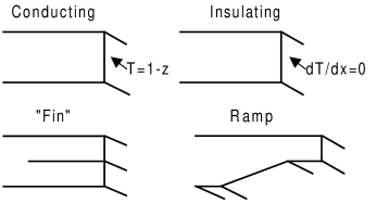
Figure 1: Four lateral sidewall boundary conditions utilized in the numerical simulations. The two thermal boundary conditions are conducting and insulating whereas the fin and ramp represent geometric conditions employed in experiments.

In experiment, however, small sidewall thermal forcing can have a significant effect upon the resulting patterns and, as a result, finned boundaries have been employed Daviaud and Pocheau (1989); de Bruyn et al. (1996); Pocheau and Daviaud (1997). These are formed by inserting a very thin piece of paper or cardboard between the top and bottom plates near the sidewalls. This suppresses convection over the finned region ($R\sim h^{3}$ and the layer height has effectively been reduced) whereas in the bulk of the domain, i.e. the un-finned region, supercritical conditions prevail. This is accomplished numerically by extending a no-slip surface into the domain from the lateral sidewall. In all of our simulations we have chosen the vertical position of the fin to be $z=0.5$ but this is not necessary. The result is that the supercritical portion of the convection layer is bounded by a subcritical region of the same fluid and hence with the same material properties. An additional effect is that the mean flow may extend into the finned region which presents an interesting scenario for exploring the effect of mean flows upon pattern dynamics that has been investigated both experimentally and theoretically by Pocheau and Daviaud  Daviaud and Pocheau (1989); Pocheau and Daviaud (1997) and is discussed further below.

The sidewalls can also have an orienting effect and ramped boundaries have been used as a “soft boundary” Kramer et al. (1982) in an effort to minimize this. By gradually decreasing the plate separation as the lateral sidewall is approached the convection layer eventually becomes critical and then increasingly subcritical. Using the spectral element algorithm we are able to investigate arbitrary ramp shapes: we have chosen to investigate the precise radial ramp utilized in recent experiments Bajaj et al. (1999); Ahlers et al. (2001) on a cylindrical convection layer. Again the mean flow is able to extend into the subcritical region.

Perhaps the most common method employed experimentally to reduce the influence of sidewalls is to use a large aspect ratio $\Gamma$, where $\Gamma=r/h$ in a cylindrical domain where $r$ is the radius and $\Gamma=L/h$ in a square domain where $L$ is the length of side. Experiments can attain aspect ratios as large as $\sim 500$. However, the majority of large aspect ratio experiments are for $\Gamma\lesssim 100$. We have performed numerical simulations using the spectral element algorithm for $\Gamma\sim 60$ as shown in Fig. 2.

The top panel in Fig. 2 illustrates the convection pattern present for the parameters of the classic paper Ahlers (1974) where flow visualization was not possible. Although the simulation has only been performed for a short time $t_{f}\sim 100\tau_{v}$ it appears that a slow process of domain coarsening Cross and Tu (1995) is occurring. The bottom of Fig. 2 illustrates the time dependent spatiotemporal chaotic state of spiral defect chaos Morris et al. (1993). These, and other, interesting large aspect ratio problems can now be addressed through the use of numerical simulation.

Heuristically, using the spectral element algorithm on an IBM SP parallel supercomputer, it is our experience that it is practical to perform full numerical simulations for aspect ratios $\Gamma\sim 30$ for simulation times of $t_{f}\sim\tau_{h}$ (36 hours on 64 processors), where $\tau_{h}$ is the horizontal diffusion time for heat ${\tau}_{h}={\Gamma}^{2}{\tau}_{v}$, and $\Gamma\sim 60$ for $t_{f}\sim 300\tau_{v}$ (36 hours on 256 processors) for $\epsilon\lesssim 1$, $0.5\lesssim\sigma\lesssim 10$, $\Delta t\approx 0.01$, and approximately cubic shaped spectral elements with an edge length of unity and $11^{th}$ order polynomial expansions (where $\epsilon=(R-R_{c})/R_{c}$ and $R_{c}$ is the critical value of the Rayleigh number). Of course for smaller domains the computational requirements significantly decrease.

A major benefit of numerical simulations is that a complete knowledge of the flow field is produced. For example, we have first used this to address a long standing open question concerning chaos in small cylindrical domains. The existence of a power-law behavior in the fall-off of the power spectral density derived from a time series of the Nusselt number was not understood Ahlers (1974). The Nusselt number, $N(t)$, is a global measurement of the temperature difference across the fluid layer. In cryogenic experiments very precise measurements of $N(t)$ are possible Ahlers (1974); Ahlers and Behringer (1978); Ahlers and Walden (1980); Libchaber and Maurer (1978), however the flow field can not be visualized easily. Subsequent room temperature experiments using compressed gasses allowed flow visualization at the expense of precise measurements of the Nusselt number Pocheau et al. (1985); Croquette et al. (1986); Pocheau (1989).

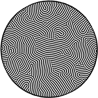
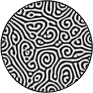
Figure 2: Numerical simulations of two large-aspect-ratio cylindrical convection layers. The pattern is illustrated by contours of the thermal perturbation, dark regions represent cool descending fluid and light regions warm ascending fluid. Both simulations are initiated from random thermal perturbations and the lateral sidewalls are insulating. (Top) $\Gamma=57$, $\sigma=2.94$, $R=2169.2$ and $t=74\tau_{v}$. (Bottom) A spiral defect chaos state, $\Gamma=30$, $\sigma=1.0$, $R=2950$ and $t=254\tau_{v}$.

By performing long-time simulations, on the order of many horizontal diffusion times, for the same parameters in cylindrical domains with $\sigma=0.78$ and for a range of $\epsilon$, with realistic boundary conditions, we had access to both precise measurements of the Nusselt number, Fig. 3, and flow visualization, Fig. 4, allowing us to resolve the issue Paul et al. (2001). Conducting sidewalls were used and all simulations were initiated from small, $\delta T\approx 0.01$, random thermal perturbations. Flow visualization of the simulations represented in Fig. 3 display a rich variety of dynamics similar to what was observed in the room temperature experiments. Using simulation results, the particular dynamical events responsible for the $N(t)$ signature were identified. The power-law behavior was found to be caused by the nucleation of dislocation pairs and roll pinch-off events. Additionally, the power spectral density was found to decay exponentially for large frequencies as expected for time-continuous deterministic dynamics. The large frequency regime was not accessible to experiment because of the presence of the noise floor.

Figure 3: Plots of the dimensionless heat transport N(t) for reduced Rayleigh number $\epsilon=0.557,0.614,0.8,1.0,1.5$, and $3.0$, labelled (i-vi) respectively ($\Gamma=4.72$). For cases (i-v), $\Delta t=0.01$, and for case (vi), $\Delta t=0.005$ ($\Delta t$ is the time step).

III Role of mean flow

The mean flow present in these flow fields, and in general for $\sigma\lesssim 1$, plays an important role in theory Newell et al. (1990); Cross and Newell (1984) yet it is not possible to measure or visualize the mean flows in the current generation of experiments. In our simulations, however, we can quantify and visualize the mean flow.

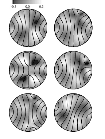
Figure 4: Flow visualization showing the pattern (solid dark lines) and shaded contours of the vorticity potential, $\zeta$, for $\epsilon=0.614$ labelled ii) in Fig 3 ($\Gamma=4.72$). Dark regions corresponding to negative vorticity generate clockwise mean flow and light regions to a positive vorticity generating a counter clockwise mean flow. The dark solid lines are zeros of the thermal perturbation at mid-depth illustrating the outline of the convection rolls. From top to bottom and left to right the panels are for $t=600,605,630,650,735,785$. The dislocations glide toward the right wall focus (shown here); during the next half period, the dislocations glide to the left wall focus. This left and right alternation continues for the entire simulation.

The mean flow field, $\vec{U}(x,y)$, is the horizontal velocity integrated over the depth and originates from the Reynolds stress induced by pattern distortions. Recalling the fluid equations, Eqs. (1) and (3), it is evident that the pressure is not an independent dynamic variable. The pressure is determined implicitly to enforce incompressibility,

$$\nabla^{2}p=-\sigma^{-1}\vec{\nabla}{\scriptscriptstyle\stackrel{{\scriptstyle\bullet}}{{{}}}}\left[\left(\vec{u}{\scriptscriptstyle\stackrel{{\scriptstyle\bullet}}{{{}}}}\vec{\nabla}\right)\vec{u}\right]+R\partial_{z}T.$$ (4)

Focussing on the nonlinear Reynolds stress term and rewriting the pressure as $p=p_{o}(x,y)+\bar{p}(x,y,z)$ yields,

$$p_{o}(x,y)\sim\sigma^{-1}\int dx^{\prime}dy^{\prime}\ln\left(1/\left|r-r^{\prime}\right|\right)\left<\vec{\nabla}^{\prime}{\scriptscriptstyle\stackrel{{\scriptstyle\bullet}}{{{}}}}\left[\left(\vec{u}{\scriptscriptstyle\stackrel{{\scriptstyle\bullet}}{{{}}}}\vec{\nabla}\right)\vec{u}\right]\right>_{z}.$$ (5)

In Eq. (5) the $\ln(1/|r-r^{\prime}|)$ is not exact, in order to be more precise the finite system Green’s function would be required. However, the long range behavior persists. This gives a contribution to the pressure that depends on distant parts of the convection pattern. The Poiseuille-like flow driven by this pressure field subtracts from the Reynolds stress induced flow leading to a divergence free horizontal flow that can be described in terms of a vertical vorticity.

The mean flow is important not because of its strength; under most conditions the mean flow is substantially smaller than the magnitude of the roll flow making it extremely difficult to quantify experimentally. The mean flow is important because it is a nonlocal effect acting over large distances (many roll widths) and changes important general predictions of the phase equation Cross and Newell (1984). The mean flow is driven by roll curvature, roll compression and gradients in the convection amplitude. The resulting mean flow advects the pattern, giving an additional slow time dependence.

The mean flow present in the simulation flow fields, $\vec{U}_{s}(x,y)$, is formed by calculating the depth averaged horizontal velocity,

$$\vec{U}_{s}(x,y)=\int^{1}_{0}\vec{u}_{\perp}(x,y,z)dz$$ (6)

where $\vec{u}_{\perp}$ is the horizontal velocity field. Furthermore it will be convenient to work with the vorticity potential, $\zeta$, defined as

$$\nabla^{2}_{\perp}\zeta=-\hat{z}{\scriptscriptstyle\stackrel{{\scriptstyle\bullet}}{{{}}}}\left(\vec{\nabla}_{\perp}\times\vec{U}_{s}\right)=-\omega_{z}$$ (7)

where $\omega_{z}$ is the vertical vorticity and $\nabla^{2}_{\perp}$ is the horizontal Laplacian.

Six consecutive snapshots in time for the periodic dynamics shown in Fig. 3 case ii) are illustrated in Fig. 4. One half period is displayed illustrating the nucleation of a dislocation pair and its subsequent annihilation in the opposing wall foci. The vorticity potential, $\zeta$, is shown on a grey scale: dark regions represent negative vorticity and light regions represent positive vorticity which will generate a clockwise and a counter clockwise rotating mean flow, respectively. The quadrupole spatial structure of $\zeta$ in the first panel, i.e. four lobes of alternating positive and negative vorticity with one lobe per quadrant, generates a roll compressing mean flow that pushes the system closer to a dislocation pair nucleation event. During dislocation climb and glide the spatial structure of the vorticity potential is more complicated until the pan-am pattern is reestablished in final panel and a quadrupole structure of vorticity is again formed and the process repeats. The dislocations alternate gliding left and right resulting is a slight rocking back and forth of the entire pattern with each half period which is visible in the different pattern orientations in the first last panels. This alternation persists for the entire simulation.

A numerical investigation of the importance of the mean flow for this small cylindrical domain was performed by implementing the ramped and finned boundary conditions. In all of these simulations the bulk region of constant $R$ extended out to a radius $r_{0}=4.72$. In the finned case a fin at half height occupied the region $4.72\leq r\leq 7.66$. In the ramped case a radial ramp in plate separation was given by,

$$h(r)=\left\{\begin{array}[]{ll}1,&\mbox{$r<r_{0}$}\\ 1-{\delta_{r}}\left[1-\cos\left(\frac{r-r_{0}}{r_{1}-r_{0}}\pi\right)\right],&\mbox{$r\geq r_{0}$}\end{array}\right.$$ (8)

where $r_{0}=4.72$, $r_{1}=10.0$, and $\delta=0.15$.

The different mean wavenumber behavior (using the Fourier methods discussed in Morris et al. (1993)) exhibited in these three different cases is shown in Fig. 5. As illustrated in Fig. 6 the behavior of the vorticity potential suggests an explanation. In the simulations with a rigid sidewall, not ramped or finned, the vorticity potential generates a mean flow that enhances roll compression, as described above. In the case of the finned and ramped boundaries the vorticity potential and the resulting mean flow are being generated by gradients in the convection amplitude and are largely situated away from the bulk of the domain. Furthermore, the mean flow generated is strongest in the subcritical finned or ramped region away from the convection rolls. This is demonstrated by comparing the average value of the mean flow over a fraction of the bulk of the domain, $r\leq 1$, where it was found that $\bar{U}_{s}=$ 0.23, 0.09, and 0.02 for the rigid, finned and ramped domains, respectively, and that the maximum flow field velocity is $|\vec{u}|\approx 10$.

Figure 5: Mean pattern wavenumber measurements for a cylindrical convection layer, $r_{0}=4.72$, with rigid sidewalls ($\Box$), fin ($\circ,r_{1}=7.66$) and a spatial ramp in plate separation ($\diamond,r_{1}=10.0$, $r_{c}=7.34$, and $\delta=0.15$). In all three cases the sidewalls are perfectly conducting and $\sigma=0.78$. For reference, solid lines labelled E, N, and SV indicate the approximate location of the Eckhaus, Neutral and Skewed Varicose stability boundaries for an infinite layer straight parallel convection rolls. All patterns represented are time independent.

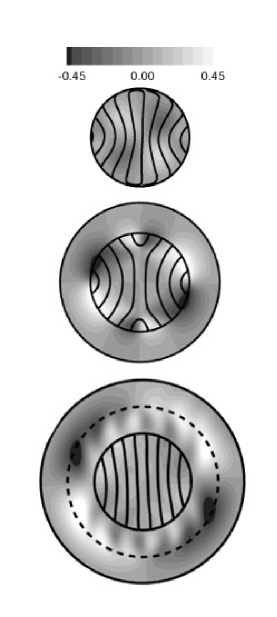
Figure 6: Convection pattern and shaded contours of the vorticity potential, $\zeta$, for a cylindrical convection layer, $r_{0}=4.72$, with rigid sidewalls, fin ($r_{1}=7.66$) and a spatial ramp in plate separation ($r_{1}=10.0$, $r_{c}=7.34$ and marked with a dashed line, and $\delta=0.15$) shown top, middle and bottom, respectively. The convection pattern is illustrated by plotting zero contours of the thermal perturbation. In all three cases the sidewalls are perfectly conducting, $\sigma=0.78$ and $R=2804$.

It is attractive to pursue the case of a radial ramp in plate separation because the variation in the convective amplitude caused by the ramp can be determined analytically and the influence of a mean flow upon nearly straight rolls can be quantified Paul et al. (2002). Usually the mean flow can only be determined once the texture is known and it is hard to calculate because of defects acting as sources, in addition to the regions of smooth distortions.

Near threshold an explicit expression for the mean flow, $\vec{U}$, that advects the convection pattern is Cross and Newell (1984)

$$\vec{U}(x,y)=-\gamma\vec{k}\vec{\nabla}_{\perp}{\scriptscriptstyle\stackrel{{\scriptstyle\bullet}}{{{}}}}\left(\vec{k}|A|^{2}\right)-\vec{\nabla}_{\perp}p_{o}(x,y)$$ (9)

where $\gamma$ is a coupling constant given by $\gamma=0.42{\sigma}^{-1}(\sigma+0.34)(\sigma+0.51)^{-1}$, $|A|^{2}$ is the convection amplitude normalized so that the convective heat flow per unit area relative to the conducted heat flow at $R_{c}$ is $|A|^{2}R/R_{c}$, $p_{o}$ is the slowly varying pressure (see Eq. (5)) and $\vec{\nabla}_{\perp}$ is the horizontal gradient operator. The vertical vorticity is then given by the vertical component of the curl of Eq. (9),

$${\omega}_{z}=\hat{z}{\scriptscriptstyle\stackrel{{\scriptstyle\bullet}}{{{}}}}\left(\vec{\nabla}_{\perp}\times\vec{U}\right)=-\gamma\hat{z}{\scriptscriptstyle\stackrel{{\scriptstyle\bullet}}{{{}}}}\vec{\nabla}_{\perp}\times\left[\vec{k}\vec{\nabla}_{\perp}{\scriptscriptstyle\stackrel{{\scriptstyle\bullet}}{{{}}}}\left(\vec{k}|A|^{2}\right)\right].$$ (10)

Consider a cylindrical convection layer with a radial ramp in plate separation containing a field of x-rolls given by $\vec{k}=k_{o}\hat{x}$. The amplitude can be represented for large $\epsilon_{o}$, using an adiabatic approximation, as $|A|^{2}=\epsilon(r)/g_{o}$ for $\epsilon>0$ and $|A|^{2}=0$ for $\epsilon(r)<0$ as shown in Fig. 7, making the amplitude a function of radius only $|A|^{2}=f(r)$.

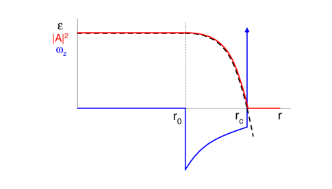
Figure 7: A schematic illustrating the radial variation, for purely adiabatic conditions, of $\epsilon$ (dashed line), $|A|^{2}$ (solid line), and $\omega_{z}$ (solid line with arrow) for a cylindrical convection layer with a radial ramp in plate separation. Labelled $r_{0}$ and $r_{c}$ are the radial values where the ramp begins and where the ramp yields critical conditions, respectively. Note that for $r>r_{c}$, $|A|^{2}=0$ in the adiabatic approximation.

Inserting $|A|^{2}=f(r)$ into Eq. (10) yields, after some manipulation, the following expression for the vertical vorticity,

$${\omega}_{z}=\frac{\gamma{k_{o}}^{2}}{2}\left[\frac{d^{2}|A|^{2}}{dr^{2}}-\frac{1}{r}\frac{d|A|^{2}}{dr}\right]\sin 2\theta.$$ (11)

The vorticity generated by the amplitude variation caused by the ramp is also shown in Fig. 7: there is a negative vorticity for $r_{0}<r<r_{c}$ and then a delta function spike of positive vorticity at $r_{c}$. To correct for nonadiabaticity and to smooth $|A(r)|^{2}$ near $r_{c}$, the one-dimensional time independent amplitude equation Newell and Whitehead (1969) is solved,

$$0=\epsilon(r)A+{{\xi}_{o}}^{2}{\cos}^{2}{\theta}\frac{\partial^{2}A}{\partial r^{2}}-g_{o}|A|^{2}A,$$ (12)

where ${{\xi}_{o}}^{2}=0.148$, $g_{o}=(0.6995-0.0047\sigma^{-1}+0.0083\sigma^{-2})$ and $\epsilon(r)$ is determined by

$$\epsilon(r)=\left\{\begin{array}[]{ll}\epsilon_{o},&\mbox{$r<r_{0}$}\\ \epsilon_{o}(h^{3}-h_{c}^{3})/(1-h_{c}^{3}),&\mbox{$r\geq r_{0}$}\end{array}\right.$$ (13)

where $h_{c}=h(r_{c})$. Equation (12) is solved numerically using the boundary conditions $\partial_{r}A=0$ at $r=0$, and $A=0$ at $r=r_{1}$.

To compare these analytical results with simulation we have chosen to investigate a large-aspect-ratio cylinder with a gradual radial ramp, defined by Eq. (8), given by the parameters: $r_{0}=11.31$, $r_{1}=20.0$, $\delta_{r}=0.036$, and $\sigma=0.87$. For small $\epsilon$ the amplitude $A^{2}(r)$ is unable to adiabatically follow the ramp, this nonadiabaticity results in a deviation from $\epsilon(r)/g_{o}$ as shown in Fig. 8a. However, as $\epsilon_{0}$ increases the amplitude $A^{2}(r)$ follows $\epsilon(r)/g_{o}$ adiabatically almost over the entire ramp except for a small kink at $r_{c}$. The structure of $\omega_{z}$ depends upon this adiabaticity and is shown in Fig. 8b where we have used the solution to Eq. (12) at $\theta=\pi/4$ in Eq. (11). This is not strictly correct since the non-adiabaticity of the amplitude is $\theta$ dependent which will induce higher angular modes of the vorticity not given by Eq. (11). However, the calculation should give a good approximation to the main $\sin 2\theta$ component of the vorticity. It is evident from Fig. 8b that the vertical vorticity, calculated from the simulation results as an angular average weighted by $\sin 2\theta$ has an octupole angular dependence (octupole in the sense of an inner and outer quadrupole) and is well approximated by theory without any adjustable parameters.

The mean flow generated by these vorticity distributions is determined by solving Eq. (10) with the boundary condition $\zeta(r_{1})=0$. The vorticity potential is related to the mean flow in polar coordinates by $(U_{r},U_{\theta})=(r^{-1}\partial_{\theta}\zeta,-\partial_{r}\zeta)$. The vorticity potential is expanded radially in second order Bessel functions while maintaining the $\sin 2\theta$ angular dependence. Of particular interest is the mean flow perpendicular to the convection rolls, $U_{r}(\theta=0)$ or equivalently $U_{x}(y=0)$, which is shown in Fig. 8c. Again the simulation results compare well with theory even in the absence of adjustable parameters.

Figure 8: Panel (a) shows the solution of Eq. (12) plotted as $A^{2}(r)$, shown for comparison is $\epsilon(r)/g_{o}$. Panel (b) compares the vertical vorticity found analytically from Eq. (12) with an angular average, weighted by $\sin 2\theta$, of the vertical vorticity from simulation. Panel (c) compares the mean flow found analytically from Eq. (7) with the mean flow from simulation. Parameters are $r_{0}=11.31$, $r_{c}=13.20$, $r_{1}=20.0$, $\delta_{r}=0.036$, $\sigma=0.87$ and $\epsilon_{o}=0.025$.

To make the connection between mean flow and wavenumber quantitative it is noted that the wavenumber variation resulting from a mean flow across a field of x-rolls can be determined from the one-dimensional phase equation,

$$U\partial_{x}\phi=D_{\parallel}\partial_{xx}\phi$$ (14)

where the wavenumber is the gradient of the phase, $k=\partial_{x}\phi$, $D_{\parallel}=\xi_{o}^{2}\tau_{o}^{-1}$, and $\tau_{o}^{-1}=19.65\sigma(\sigma+0.5117)^{-1}$ Cross and Hohenberg (1993). Figure 9a illustrates the wavenumber variation for a large-aspect-ratio simulation, $k(r)$ for $r\leq r_{0}$, and makes evident the roll compression, $k(r=0)>k(r_{0})$. Figure 9b compares the mean flow calculated from simulation to the predicted value of the mean flow required to produce the wavenumber variation shown in Fig. 9a. The agreement is good and the discrepancy near $r_{0}$, which is contained within one roll wavelength from where the ramp begins, is expected because the influence of the ramp was not included in Eq. (14). This illustrates quantitatively that is in indeed the mean flow that compresses the rolls in the bulk of the domain.

Figure 9: Panel (a), the variation in the local wavenumber along the positive x-axis, or equivalently $k(r)$ at $\theta=0$. Panel (b), a comparison of the mean flow from simulation (solid line) with the predicted value (dashed line) calculated from Eq. (14) using the wavenumber variation from panel (a). Simulation parameters, $r_{0}=11.31$, $r_{1}=20$, $\delta_{r}=0.036$, $\sigma=0.87$ and $\epsilon=0.171$.

Finally, to better understand the connection between mean flow and pattern dynamics, especially that of spatiotemporal chaotic states exhibiting both temporal chaos as well as spatial disorder, we apply a novel numerical procedure to eliminate mean flow from the fluid equation, Eq. (1), thereby evolving the dynamics of an artificial fluid with no explicit contributions from mean flow. In this way, we can then obtain quantitative comparisons between the patterns generated by this artificial fluid with mean flow quenched and by the original fluid equation.

We have applied this procedure to study spiral defect chaos (see bottom of Fig. 2) Morris et al. (1993). Numerous attempts have been made to understand how a spiral defect chaos state is formed and how it is sustained. For example, experiments Assenheimer and Steinberg (1993); Assenheimer and Steinberg (1994) have found that spirals transition to targets when the Prandtl number is increased. Owing to the fact that the magnitude of mean flow is inversely proportional to the Prandtl number, c.f. Eq. (9), it was believed that spiral defect chaos is a low Prandtl number phenomenon for which mean flow is essential to their dynamics. This is supported by studies of convection models based on the generalized Swift-Hohenberg equation Xi et al. (1993a, b); Xi and Gunton (1995), where spiral defect chaos is not observed unless a term corresponding to mean flow is explicitly coupled to the equation. However, these observations are by themselves insufficient. For example, there are many other effects in the fluid equations that grow towards low Prandtl numbers, and there could be limitations in the Swift-Hohenberg modelling. We have applied our numerical procedure to this case to explicitly confirm the role of mean flow in the dynamics of spiral defect chaos.

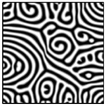
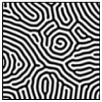
Figure 10: Spiral defect chaos (left) and angular textures (right) obtained by quenching mean flow. The left panel is at $t=152\tau_{v}$ and displays the pattern upon which the mean flow is quenched, the right panel is at $t=320\tau_{v}$. In both cases, $R=2950,\sigma=1.0$ and the lateral sidewalls are insulating. We see that the spiral arms transition to angular textures when mean flow is quenched. Also, the quenched state is stationary.

Recalling that we can approximate mean flow to be the depth-averaged horizontal velocity, c.f. Eq. (6), we can first depth-average the horizontal components of the fluid equation, Eq. (1), to obtain a dynamical equation for the mean flow $\vec{U}_{s}$:

$$\sigma^{-1}\partial_{t}\vec{U}_{s}+\sigma^{-1}\int_{0}^{1}dz(\vec{u}{\scriptscriptstyle\stackrel{{\scriptstyle\bullet}}{{{}}}}\vec{\nabla})\vec{u}_{\perp}=$$ (15)

$$-\vec{\nabla}_{\perp}\int_{0}^{1}dzp+\nabla_{\perp}^{2}\vec{U}_{s}+\int_{0}^{1}dz\partial_{zz}\vec{u}_{\perp}.$$

In this equation, the term $-\nabla_{\perp}\int_{0}^{1}dzp$ can be absorbed into the nonlinear Reynolds stress term via Eq. (5) and so will be ignored henceforth. The resulting equation is then a diffusion equation in $\vec{U}_{s}$ with a source term $\vec{F}_{s}\equiv\int_{0}^{1}dz(\vec{u}{\scriptscriptstyle\stackrel{{\scriptstyle\bullet}}{{{}}}}\nabla)\vec{u}_{\perp}-\sigma\int_{0}^{1}dz\partial_{zz}\vec{u}_{\perp}$. If this source term were not present, then $\vec{U}_{s}$, being the solution to a diffusion equation, evolves to zero with an effective diffusivity $\sigma$, the Prandtl number. Thus, the role of $\vec{F}_{s}$ is to act as a generating source for the mean flow $\vec{U}_{s}$. Subtracting it from the fluid equation, Eq. (1), then results in the mean flow being eliminated.

In practice, we found that it is necessary to actually subtract $\vec{F}_{s}$ multiplied by a constant to ensure that the magnitude of mean flow becomes zero. This can be understood in terms of the necessity to correct for the fact that Eq. (6) is only an approximation to the flow field that advects the rolls given by

$$\vec{U}=\int_{0}^{1}dzg(z)\vec{u}_{\perp}$$ (16)

where $g(z)$ is a weighting function depending on the full nonlinear structure of the rolls. This is discussed further elsewhere Chiam et al. (2002).

We have carried out this procedure by introducing the term $\vec{F}_{s}$ to the right-hand-side of the fluid equation after a spiral defect chaotic state becomes fully developed, typically after about one horizontal diffusion time starting from random thermal perturbations as initial condition. We see that the spirals immediately, on the order of a vertical diffusion time, “straighten out” to form angular chevron-like textures; see Fig. 10. Unlike spiral defect chaos, these angular textures are stationary (with the exception of the slow motion of defects such as the gliding of dislocation pairs). Thus, we have shown that when mean flow is quenched via the subtraction of the term $\vec{F}_{s}$ from the fluid equation, spiral defect chaos ceases to exist.

We have further quantified the differences between spiral defect chaos and the angular textures. We mention here briefly one of the results: by comparing the wavenumber distribution for both sets of states, we have observed that the mean wavenumber approaches the unique wavenumber possessed by axisymmetric patterns asymptotically far away from the center Buell and Catton (1986). (The axisymmetric pattern, by symmetry, does not have mean flow components.) We discuss this as well as other results in a separate article Chiam et al. (2002).

IV Conclusion

Full numerical simulations of Rayleigh-Bénard convection in cylindrical and rectangular shaped domains for a range of aspect ratios, $5\lesssim\Gamma\lesssim 60$, with experimentally realistic boundary conditions, including rigid, finned and spatially ramped sidewalls, have been performed. These simulations provide us with a complete knowledge of the flow field allowing us to quantitatively address some interesting open questions.

In this paper we have emphasized the exploration of the mean flow. The mean flow is important in a theoretical understanding of the pattern dynamics, yet is very difficult to measure in experiment, making numerical simulations attractive to close this gap.

The mean flow is found to be important in small cylindrical domains by investigating the result of imposing different sidewall boundary conditions. Analytical results are developed for a large-aspect-ratio cylinder with a radial ramp in plate separation. Numerical results of the vertical vorticity and the mean flow agree with these predictions. Furthermore, the wavenumber behavior predicted using the mean flow in a one-dimensional phase equation also agrees with the results of simulation. This allows extrapolation of the analysis to larger aspect ratios.

Lastly we utilize the control and flexibility offered by numerical simulation to investigate a novel method of quenching numerically the mean flow. We apply this to a spiral defect chaos state and find that the time dependent pattern becomes time independent, angular in nature, and that the pattern wavenumber becomes larger.

These quantitative comparisons illustrate the benefit of performing numerical simulations for realistic geometries and boundary conditions as a means to create quantitative links between experiment and theory.

We are grateful to G. Ahlers for helpful discussions. This research was supported by the U.S. Department of Energy, Grant DE-FT02-98ER14892, and the Mathematical, Information, and Computational Sciences Division subprogram of the Office of Advanced Scientific Computing Research, U.S. Department of Energy, under Contract W-31-109-Eng-38. We also acknowledge the Caltech Center for Advanced Computing Research and the North Carolina Supercomputing Center.

References

- Cross and Hohenberg (1993) M. C. Cross and P. C. Hohenberg, Rev. of Mod. Phys. 65(3 II), 851 (1993).
- Fischer (1997) P. F. Fischer, J. Comp. Phys. 133, 84 (1997).
- Daviaud and Pocheau (1989) F. Daviaud and A. Pocheau, Europhysics Letters 9(7), 675 (1989).
- de Bruyn et al. (1996) J. R. de Bruyn, E. Bodenschatz, S. W. Morris, D. S. Cannell, and G. Ahlers, Rev. Sci. Instrum. 67(6), 2043 (1996).
- Pocheau and Daviaud (1997) A. Pocheau and F. Daviaud, Phys. Rev. E 55(1), 353 (1997).
- Kramer et al. (1982) L. Kramer, E. Ben-Jacob, H. Brand, and M. C. Cross, Phys. Rev. Lett. 49(26), 1891 (1982).
- Bajaj et al. (1999) K. M. S. Bajaj, N. Mukolobwiez, N. Currier, and G. Ahlers, Phys. Rev. Lett. 83(25), 5282 (1999).
- Ahlers et al. (2001) G. Ahlers, K. M. S. Bajaj, N. Mukolobwicz, and J. Oh, unpublished (2001).
- Ahlers (1974) G. Ahlers, Phys. Rev. Lett. 33(20), 1185 (1974).
- Cross and Tu (1995) M. C. Cross and Y. Tu, Phys. Rev. Lett. 75(5), 834 (1995).
- Morris et al. (1993) S. W. Morris, E. Bodenschatz, D. S. Cannell, and G. Ahlers, Phys. Rev. Lett. 71(13), 2026 (1993).
- Ahlers and Behringer (1978) G. Ahlers and R. P. Behringer, Phys. Rev. Lett. 40, 712 (1978).
- Ahlers and Walden (1980) G. Ahlers and R. W. Walden, Phys. Rev. Lett. 44(7), 445 (1980).
- Libchaber and Maurer (1978) A. Libchaber and J. Maurer, J. Physique Lett. 39, 369 (1978).
- Pocheau et al. (1985) A. Pocheau, V. Croquette, and P. Le Gal, Phys. Rev. Lett. 55(10), 1094 (1985).
- Croquette et al. (1986) V. Croquette, P. Le Gal, and A. Pocheau, Phys. Scr. T13, 135 (1986).
- Pocheau (1989) A. Pocheau, J. Phys. France 50, 2059 (1989).
- Paul et al. (2001) M. R. Paul, M. C. Cross, P. F. Fischer, and H. S. Greenside, Phys. Rev. Lett. 87(15), 154501 (2001).
- Newell et al. (1990) A. C. Newell, T. Passot, and M. Souli, J. Fluid Mech. 220, 187 (1990).
- Cross and Newell (1984) M. C. Cross and A. C. Newell, Physica D 10, 299 (1984).
- Paul et al. (2002) M. R. Paul, M. C. Cross, and P. F. Fischer, Phys. Rev. E 66, 046210 (2002).
- Newell and Whitehead (1969) A. C. Newell and J. A. Whitehead, J. Fluid Mech. 38(2), 279 (1969).
- Assenheimer and Steinberg (1993) M. Assenheimer and V. Steinberg, Phys. Rev. Lett. 70(25), 3888 (1993).
- Assenheimer and Steinberg (1994) M. Assenheimer and V. Steinberg, Nature 367 (1994).
- Xi et al. (1993a) H.-w. Xi, J. D. Gunton, and J. Viñals, Phys. Rev. Lett. 71(13), 2030 (1993a).
- Xi et al. (1993b) H.-w. Xi, J. D. Gunton, and J. Viñals, Phys. Rev. E 47(5), 2987 (1993b).
- Xi and Gunton (1995) H. Xi and J. D. Gunton, Phys. Rev. E 52(5), 4963 (1995).
- Chiam et al. (2002) K.-H. Chiam, M. R. Paul, M. C. Cross, and H. S. Greenside, unpublished (2002).
- Buell and Catton (1986) J. C. Buell and I. Catton, Phys. Fluids 29, 23 (1986).