Drag Reduction by Polymers in Turbulent Channel Flows:
Energy Redistribution Between Invariant Empirical Modes.

Abstract

We address the phenomenon of drag reduction by dilute polymeric additive to turbulent flows, using Direct Numerical Simulations (DNS) of the FENE-P model of viscoelastic flows. It had been amply demonstrated that these model equations reproduce the phenomenon, but the results of DNS were not analyzed so far with the goal of interpreting the phenomenon. In order to construct a useful framework for the understanding of drag reduction we initiate in this paper an investigation of the most important modes that are sustained in the viscoelastic and Newtonian turbulent flows respectively. The modes are obtained empirically using the Karhunen-Loéve decomposition, allowing us to compare the most energetic modes in the viscoelastic and Newtonian flows. The main finding of the present study is that the spatial profile of the most energetic modes is hardly changed between the two flows. What changes is the energy associated with these modes, and their relative ordering in the decreasing order from the most energetic to the least. Modes that are highly excited in one flow can be strongly suppressed in the other, and vice versa. This dramatic energy redistribution is an important clue to the mechanism of drag reduction as is proposed in this paper. In particular there is an enhancement of the energy containing modes in the viscoelastic flow compared to the Newtonian one; drag reduction is seen in the energy containing modes rather than the dissipative modes as proposed in some previous theories.

I Introduction

“Drag reduction” refers to the interesting observation that the addition of a few tens of parts per million (by weight) of long-chain polymers to turbulent fluids can bring about a reduction of the friction drag by up to 80% 00SW . Obviously, the phenomenon has far reaching practical implications besides being challenging from the fundamental point of view. In spite of intense interest for an extended period of time 69Lu ; 75Virk ; 90Ge , Sreenivasan and White 00SW recently concluded that “it is fair to say that the extensive - and continuing - activity has not produced a firm grasp of the mechanisms of drag reduction”. In this paper we want to advance on the basis of recent Direct Numerical Simulation of model viscoelastic hydrodynamic equations 97THKN ; 98DSB ; 00ACP ; 02ACP . Such DNS show unequivocally that drag reduction is reproduced by model equations like the FENE-P model. From the theoretical point of view this is significant, since it indicates that the phenomenon is included in the solutions of the model equations. Understanding drag reduction then becomes a usual challenge of theoretical physics.

Our thinking here is motivated in part by a recent analysis of the stability of laminar channel flows subject to space dependent effective viscosity 01GLP ; 02GLP . It turned out the even small viscosity gradients can lead to a giant stabilization of the most unstable modes, both for primary and secondary instabilities. In these cases one can understand the phenomenon completely by examining the energy budget of the putative unstable modes and their interaction with the mean flow; the most important observation had been that it is the the existence of viscosity gradients positioned at a strategic distance from the wall which is crucial for the existence of a large effect. It seems desirable to do something similar for the viscoelastic turbulent flows as well (in which the space dependent effective viscosity arises due to differential stretching of the polymers). But alas, in distinction from primary and secondary instabilities, where it is obvious which are the relevant modes, for the turbulent flow these are not known apriori. We therefore decided to first initiate a systematic study of the empirical modes that are sustained in the turbulent flow, and then to discuss their interaction with the mean flow and with the polymeric additive, their stabilization or destabilization when we compare the viscoelastic to the Newtonian flow, and their energy budget. In this paper we present the first results of this study.

We will demonstrate that we can determine with reasonable accuracy at least the first thirty most energetic modes that are sustained in the turbulent flow, for both the FENE-P and the Navier-Stokes equations (run at the same friction Reynolds number, and see below for details). These modes can be arranged in descending order according to their relative energy. Unexpectedly we find that the nature of the most relevant modes is unchanged in the two cases. On the other hand the energies associated with the modes and their relative ordering are changed; some modes that are energetic in one flow are strongly suppressed (their energy decreases by a factor of 4) in the other flow, and vice versa. Most importantly, the few most energetic modes of the viscoelastic flow contain a lot more energy that the same number of most energetic Newtonian modes. We propose therefore that drag reduction should be understood by examining the dynamics and relative stability of the energy containing modes rather than focusing only on the dissipative end of the spectrum, as proposed for example in 90Ge .

In Sects. II A and B we summarize the FENE-P equations and the numerical approach. In Sect. II.3 we present the essential results regarding the observation of drag reduction. In Sect. III we review the Karhunen-Loéve method for determining the best empirical modes, and apply it to the problem at hand. In Sect. IV we discuss the results, demonstrate the invariance of the modes, and present the relative ordering. Sect. V is devoted to a discussion of the findings and of the road ahead.

II Equations of Motion and Direct Numerical Simulations

II.1 The FENE-P model for dilute polymers

The addition of a dilute polymer to a Newtonian fluid gives rise to an extra stress tensor ${\bm{{\mathcal{T}}}}({\bm{r}},t)$ which affects the Navier-Stokes equations:

$$\frac{\partial{\bm{u}}}{\partial t}+({\bm{u}}\cdot{\bm{\nabla}}){\bm{u}} = -{\bm{\nabla}}p+\nu_{\rm s}\nabla^{2}{\bm{u}}+{\bm{\nabla}}\cdot{\bm{{\mathcal{T}}}}\ ,$$

$${\bm{\nabla}}\cdot{\bm{u}} = 0\ .$$ (1)

Here ${\bm{u}}({\bm{r}},t)$ is the solenoidal velocity field, $p({\bm{r}},t)$ is the pressure and $\nu_{s}$ is the viscosity of the neat fluid. The additional stress tensor ${\bm{{\mathcal{T}}}}$ is not known exactly, and needs to be modeled. There are a number of competing derivations, see 87BCAH ; 94BE . In our work we adopt the FENE-P model that is derived on the basis of a dumbbell model for the polymers 87BCAH ; 94BE and is known to reproduce the phenomenon of drag reduction. In this model ${\bm{{\mathcal{T}}}}$ is determined by the “polymer conformation tensor” ${\bm{R}}$ according to

$${\bm{{\mathcal{T}}}}({\bm{r}},t)=\frac{\nu_{\rm p}}{\tau_{\rm p}}\left[\frac{f({\bm{r}},t)}{\rho_{0}^{2}}{\bm{R}}({\bm{r}},t)-{\bm{1}}\right]\ .$$ (2)

Here ${\bm{1}}$ is the unit tensor, $\nu_{\rm p}$ is a viscosity parameter, $\tau_{\rm p}$ is a relaxation time for the polymer conformation tensor and $\rho_{0}$ is a parameter which in the derivation of the model stands for the rms extension of the polymers in equilibrium. The function $f({\bm{r}},t)$ limits the growth of the trace of ${\bm{R}}$ to a maximum value $\rho_{\rm m}$:

$$f({\bm{r}},t)\equiv\frac{\rho_{\rm m}^{2}-\rho_{0}^{2}}{\rho_{\rm m}^{2}-R_{\gamma\gamma}({\bm{r}},t)}\ .$$ (3)

The model is closed by the equation of motion for the conformation tensor which reads

$$\frac{\partial R_{\alpha\beta}}{\partial t} + ({\bm{u}}\cdot{\bm{\nabla}})R_{\alpha\beta}=\frac{\partial u_{\alpha}}{\partial r_{\gamma}}R_{\gamma\beta}+R_{\alpha\gamma}\frac{\partial u_{\gamma}}{\partial r_{\beta}}$$ (4)

$$- \frac{1}{\tau_{\rm p}}\left[f({\bm{r}},t)R_{\alpha\beta}-\rho_{0}^{2}\delta_{\alpha\beta}\right]\ .$$

The model is derived by assuming that the polymer can be characterized completely by an end-to-end vector distance. Nevertheless the resulting equations could be written on the basis of plausible arguments including up to quadratic terms in gradients and available tensors. For our purposes the accuracy of the model in reproducing quantitatively all the phenomena of turbulence in viscoelastic fluids is not an issue of concern. We are mainly interested in the fact that these equations were simulated on the computer in a channel geometry and exhibited the phenomenon of drag reduction as discussed below. Our aim is to understand drag reduction within the FENE-P model.

II.2 Direct Numerical Simulations

A simple flow geometry which exhibits the phenomenon of drag reduction is channel flow between two parallel planes, separated by the distance $2H$ in the $y$-direction, see Fig. 1. The computational domain is periodic in the two directions parallel to the wall (streamwise $x$, spanwise $z$).

Figure 1: Geometry of the channel flow between two parallel planes separated by $2H$ in the $y$ direction. The mean velocity $\overline{{\bm{U}}}(y)$ is oriented along the $x$ axis (streamwise direction). The three-dimensional velocity fluctuations are space-homogeneous in the $x-z$ plane, where $z$ is usually called the span-wise direction. It is customary to use the Fourier decomposition in this plane; ${\bm{q}}=(q_{x},q_{z})$ is the corresponding two-dimensional wave vector.

The Navier-Stokes equation (1) is written in terms of wall-normal component of velocity $u_{y}({\bm{r}},t)$ and the vorticity $\omega_{y}({\bm{r}},t)$, where ${\bm{\omega}}={\bm{\nabla}}\times{\bm{u}}$,

$$\frac{\partial u_{y}}{\partial t}+({\bm{u}}\cdot{\bm{\nabla}})u_{y} = -\frac{\partial p}{\partial y}+\nu_{s}\nabla^{2}u_{y}+\nabla_{\beta}{\mathcal{T}}_{\beta y}$$

$$\frac{\partial\omega_{y}}{\partial t}+\left({\bm{u}}\cdot{\bm{\nabla}}\right)\omega_{y} = \left({\bm{\omega}}\cdot{\bm{\nabla}}\right)u_{y}+\nu_{\rm s}\nabla^{2}\omega_{y}$$ (5)

$$+\epsilon_{y\beta\gamma}\nabla_{\beta}\nabla_{\delta}{\mathcal{T}}_{\delta\gamma}$$

with $\epsilon_{\alpha\beta\gamma}$ the fully antisymmetric Levi-Civita tensor. Given $u_{y}$ and $\omega_{y}$, the components of the velocity field in the two directions parallel to the $x-z$ plane follow from the continuity equation and the definition of $\omega_{y}$,

$${\bm{\nabla}}_{\parallel}\cdot{\bm{u}}_{\parallel}=-\frac{\partial u_{y}}{\partial y} ,\qquad {\bm{\nabla}}_{\parallel}\times{\bm{u}}_{\parallel}=\omega_{y},$$ (6)

where the subscript $\parallel$ denotes projection of vectors on the $x-z$ plane. The system of Eqs. (II.2,6) is one of the standard formulations used for the direct numerical simulation of turbulent channel flows, since the procedure yields a solenoidal velocity field to machine accuracy.

In light of the periodicity in the $x-z$ plane, it is natural to expand the planar components of the velocity field in Fourier modes. For the wall-normal direction one uses Chebyshev polynomials. The time stepping is carried out by a mixed Crank-Nicolson/Runge-Kutta scheme for the viscous and the nonlinear terms, respectively. The integration in the normal direction is done by Chebyshev tau-method and a standard de-aliasing technique is adopted for the nonlinear terms. The typical simulations have been performed on a computational grid of $96\times 129\times 96$ nodes in a domain of dimensions $2\pi H\times 2H\times 1.2\pi H$. Turbulence is maintained by enforcing the same constant pressure gradient for the corresponding Newtonian and viscoelastic simulations.

In discussing the simulations, one notes that the channel half-height $H$ is only one of the parameters which sets up the external lengthscale. An additional important control parameter is the enforced pressure gradient at the wall, which determines the friction. Denoting by pointed brackets an average over time the friction parameter is defined as

$$\overline{\tau}_{\rm w}=H\left\langle\frac{\partial p}{\partial x}\right\rangle\ .$$ (7)

This is the basic control parameter of the flow. By considering also the overall kinematic viscosity, $\nu_{\rm f}=\nu_{\rm s}+\nu_{\rm p}$, the traditional friction Reynolds number is defined as

$${\rm Re}_{\tau}=\frac{u_{\tau}H}{\nu_{\rm f}},\qquad u_{\tau}=\sqrt{\overline{\tau}_{\rm w}}\ ,$$ (8)

where $u_{\tau}$ is the friction velocity. As customary in wall turbulence, one may introduce the inner, or viscous, length scale

$$\ell=\frac{\nu_{\rm f}}{u_{\tau}}\ .$$ (9)

The inner velocity scale $u_{\tau}$ has its counterpart bulk velocity

$$U_{0}=\frac{1}{2H}\int dy\langle u_{x}\rangle\ .$$ (10)

Correspondingly we have the outer and inner time scales $T_{0}=H/U_{0}$ and $\nu_{\rm f}/u_{\tau}^{2}$ respectively.

In the sequel all quantities are made dimensionless unless stated otherwise. Those made dimensionless with respect to the appropriate inner scale will be denoted by the superscript $+$; no special symbol is used to denote normalization by an outer scale.

Finally there are parameters associated with the polymer. Foremost is the Deborah number which is defined as the ratio of the relaxation time $\tau_{\rm p}$ and a typical time scale of the fluid motion, i.e.

$${\rm De}=\frac{\tau_{\rm p}}{T_{0}}.$$ (11)

The parameter $r_{\rm p}=\nu_{\rm p}/\nu_{\rm s}$ measures the relative viscosity of the polymers with respect to the Newtonian solvent, and the non-linear characteristics of the spring is defined in terms of the ratio $\rho_{\rm m}^{2}/\rho_{0}^{2}$.

In all our comparisons of Newtonian and viscoelastic simulations, the friction Reynolds number is kept constant, at a typical value ${\rm Re}_{\tau}=125$. The correspondence between the two flows is obtained by fixing the computational domain, and choosing for the Newtonian case a viscosity equal to the overall viscosity of the solution. The parameters chosen for all the viscoelastic simulations are ${\rm De}=25$, $\eta_{\rm p}=0.1$ and $\rho_{\rm m}^{2}/\rho_{0}^{2}=1000$.

II.3 Overview of drag reduction

In this subsection we review briefly the main results of the present simulations which demonstrate the phenomenon of drag reduction. For more detailed description, see 02ACP . The analysis presented in the following sections employs the very same DNS.

In comparing the viscoelastic and the Newtonian flows we maintain the friction Reynolds number (8) fixed. We reiterate that to achieve this we need to choose the viscosity of the Newtonian flow properly, since the viscoelastic wall stress contains a small viscoelastic contribution,

$$\overline{\tau}_{\rm w}=\nu_{\rm s}\frac{d\overline{U}}{dy}+\overline{{\mathcal{T}}}_{yx}\ .$$ (12)

The component of the extra-stress ${\mathcal{T}}_{yx}$ does not vanish on the average, contributing in our simulation about $10\%$ of the total drag.

The main observations regarding drag reductions are as follows:

(i) For a fixed mean pressure gradient at the wall, the viscoelastic flow exhibits an increased flow rate through the channel, see Fig. 2.

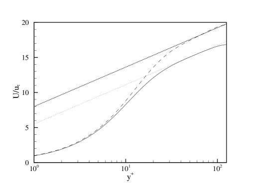
Figure 2: Mean velocity profiles for the Newtonian and for the viscoelastic simulations with ${\rm Re}_{\tau}=125$. Solid line: Newtonian. Dashed line: Viscoelastic. The straight lines represent the classical log-law, Eq. (15).

Shown there are the mean profiles in the streamwise direction, the other means vanish by symmetry:

$$\overline{U}_{x}(y) = \overline{U}(y)\equiv\langle u_{x}({\bm{r}},t)\rangle,$$ (13)

$$\overline{U}_{y}(y) = \overline{U}_{z}(y)=0\ .$$

The increase in the throughput entails an increased bulk Reynolds number,

$${\rm Re}_{\rm b}=\frac{U_{0}H}{\nu_{\rm f}}\ .$$ (14)

(ii) Some typical length scales increase in the viscoelastic flow. The data in Fig. 2 can be recast in terms of the log-law of the wall,

$$\overline{U}^{+}=\frac{1}{k}\log{y^{+}}+A,$$ (15)

where $k\simeq 0.4$ is the Von Karman constant. The constant $A$ depends on the thickness of the buffer plus viscous sub-layers, defined as the distance between the wall and the beginning of the log-region. The log-law exists equally well for the viscoelastic as for the Newtonian flow with the same $k$, but the numerical value of the constant $A$ is substantially increased in the former. This thickening of the buffer layer is directly related to the increased flow rate. The effect of thickening buffer layer can be also measured by the increase of the span-wise scale of the streamwise velocity fluctuations. Decomposing the velocity field into a mean and a fluctuating part

$$u_{\alpha}({\bm{r}},t)=\overline{U}_{\alpha}(y)+\tilde{u}_{\alpha}({\bm{r}},t),$$ (16)

one introduces the correlation tensor

$$K_{\alpha\beta}({\bm{r}},{\bm{r}}^{\prime})\equiv\langle\tilde{u}_{\alpha}({\bm{r}},t)\tilde{u}_{\beta}({\bm{r}}^{\prime},t)\rangle\ .$$ (17)

In Fig. 3 we show $K_{xx}({\bm{r}},{\bm{r}}^{\prime})$ for ${\bm{r}}=(x,y,z)$, ${\bm{r}}^{\prime}=(x,y,z+Z)$. [Note that by homogeneity $K_{xx}=K_{xx}(y,Z)$]. Fig. 3 demonstrated the increase in the span-wise correlation length of the streamwise velocity fluctuations which can be defined as

$$L_{xz}(y)\equiv\frac{1}{K_{xx}(y,0)}\int dZK_{xx}(y,Z)\ .$$ (18)

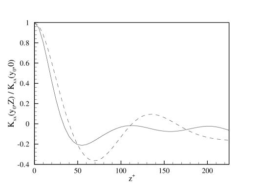
Figure 3: Two point span-wise correlation of the streamwise velocity component, $K_{xx}(y_{0},Z)/K_{xx}(y_{0},0)$: viscoelastic flow (dashed line), Newtonian flow (solid line). ${\rm Re}_{\tau}=125$, $y_{0}^{+}=7$.

(iii) Comparison of the time signals between the viscoelastic and Newtonian cases shows an alteration of the characteristic frequencies for the viscoelastic model. This corresponds quite well to the experimental data, for example of Luchik et al. Tiederman , in which a decrease of the bursting frequency is observed in drag reducing solutions. We do not reproduce these results here.

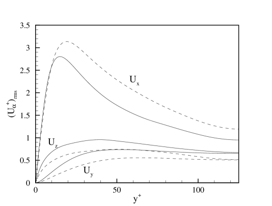
Figure 4: Velocity fluctuations, normalized by friction velocity $u_{\tau}$, for the viscoelastic (dashed line) and the Newtonian flow (solid line). In both cases, $U_{x}$, $U_{y}$ and $U_{z}$ are given by solid dashed and dotted lines, respectively.

(iv) Finally, the root mean square fluctuations change significantly as a function of $y$. Denoting

$$U_{\alpha}(y)\equiv\sqrt{\langle|\tilde{u}_{\alpha}({\bm{r}},t)|^{2}\rangle}\ ,$$ (19)

we display in Fig. 4 the $y$ dependence of the three components $\alpha=x,y,z$. The streamwise fluctuations are shown to increase with respect to the corresponding Newtonian flow, while both the span-wise and the wall-normal fluctuations decrease, in qualitative agreement with available experimental results Tiederman .

In conclusion, the FENE-P model is shown to exhibit the phenomenon of drag reduction in close similarity to experimental observations. In addition, DNS of this model provides complete information about the velocity field and the covariance tensor field ${\bm{R}}({\bm{r}},t)$ as a function of space and time. We thus feel confident that a sufficiently savvy analysis of this model and its turbulent flow pattern should provide insight into the mechanism of drag reduction.

III Analysis Using Empirical Modes

In this section we present the analysis of the difference between viscoelastic and Newtonian flows in term of the empirical modes that are sustained in the turbulent flow. In choosing a method to extract the modes we are led by the desire to find the “best” modes, and “best” in our case will mean those that are most energetic. In fluid mechanics the energy is quadratic in the field, so “best” is related to closeness in the $L^{2}$ norm. As is well known, the standard method to find best representation in $L^{2}$ norms is the Karhunen-Loéve method. The aim of the Karhunen Loéve method is to provide a set of modes that optimally decompose the field of interest, in our case the velocity field averaged over time. The approach is guaranteed to yield the best set of truncated modes, meaning that the field cannot be approximated better (in $L^{2}$ norm) by any other set of the same number of modes. The method had been applied to fluid mechanics in a number of contexts, see for example Siro1 ; Siro2 ; Holmes for details and relevant references. We first adapt the Karhunen-Loéve method to the present context, and then discuss the results of the analysis.

The core object for the analysis is the simultaneous correlation function of the velocity fluctuations which was introduced already in Eq.(17). Due to stationarity this object is time independent, and due to homogeneity in the $x$ and $z$ direction, we can write

$$K_{\alpha\beta}=K_{\alpha\beta}(x^{\prime}-x,z^{\prime}-z;y,y^{\prime})\ .$$ (20)

In the translationally invariant directions $x-z$ one cannot do better than Fourier decomposition. Accordingly we consider the partly decomposed object $\hat{Q}({\bm{q}}|y,y^{\prime})$ defined as

$$\hat{Q}({\bm{q}}|y,y^{\prime}) \equiv \frac{1}{N_{\parallel}}\sum_{{\bm{r}}_{\parallel}}K_{\alpha\beta}(x^{\prime}-x,z^{\prime}-z;y,y^{\prime})$$

$$\times\exp\{-\imath[q_{x}(x^{\prime}-x)+q_{z}(z^{\prime}-z)]\}\ .$$

We denoted the discrete two dimensional wave-vector in the $x-z$ plane as ${\bm{q}}=(q_{x},q_{z})=(\tilde{q}_{x}2\pi/\Lambda_{x},\tilde{q}_{z}2\pi/\Lambda_{z})$ where $\tilde{q}_{x},\tilde{q}_{z}$ are integers. $N_{\parallel}=N_{x}N_{z}$ and the sum is taken over the discrete set of $x-z$ points with ${\bm{r}}_{\parallel}=(j_{x}\Lambda_{x}/N_{x},j_{z}\Lambda_{z}/N_{z})$ the $x-z$ projection of ${\bm{r}}$.

The non-trivial empirical modes are obtained from the remaining dependence on $y,y^{\prime}$, for each given planar ${\bm{q}}$. The Karhunen-Loéve method consists of finding the eigenfunctions $\Psi_{\alpha\beta}({\bm{q}},p|y)$ which solve the eigenvalue equation

$$\int_{-1}^{1}\hat{Q}_{\alpha\beta}({\bm{q}}|y,y^{\prime})\Psi_{\beta}({\bm{q}},{\rm p}|y^{\prime})dy^{\prime}=E({\bm{q}},{\rm p})\Psi_{\alpha}({\bm{q}},{\rm p}|y)\ .$$ (22)

Here $E({\bm{q}},{\rm p})$ is the energy associated with the mode $({\bm{q}},{\rm p})$, ordered in decreasing energy order, with a given ${\bm{q}}$ wave-vector in the wall parallel directions, and p mode number in the $y$-direction, orthogonal to the plane walls. Denoting by ${\mathcal{E}}$ the total energy in the system, we have

$${\mathcal{E}}\equiv\int d^{3}{\bm{r}}\frac{\tilde{u}^{2}}{2}=\sum_{{\bm{q}},{\rm p}}E({\bm{q}},{\rm p}).$$ (23)

The modes labeled by $({\bm{q}},{\rm p})$ can be relabeled in order of decreasing energy by introducing an index $n$. In this notation the mode whose associated energy is $E_{n}=E({\bm{q}},{\rm p})$ are denoted by

$$\Psi_{\alpha}(n|y)\equiv\Psi_{\alpha}({\bm{q}}_{n},{\rm p_{n}}|y),$$ (24)

where $({\bm{q}}_{n},{\rm p}_{n})$ is the label of the $n^{\rm th}$ mode. It is useful to introduce also a set of fields indexed by $n$,

$$\Phi_{\alpha}(n|{\bm{r}})=\Psi_{\alpha}(n|y)\exp\left[\imath({\bm{q}}_{n}\cdot{\bm{r}}_{\parallel})\right]\ .$$ (25)

These function are orthogonal in the sense

$$\frac{1}{2N_{\parallel}}\sum_{{\bm{r}}_{\parallel}}\int_{-1}^{1}dy\Phi_{\alpha}(n|y,{\bm{r}}_{\parallel})\Phi^{*}_{\alpha}(n^{\prime}|y,{\bm{r}}_{\parallel})=\delta_{nn^{\prime}}\ .$$ (26)

The fluctuation velocity field can be now expanded in terms of these fields,

$$\tilde{u}_{\alpha}(t,{\bm{r}})=\sum_{n}a_{n}(t)\Phi_{\alpha}(n|{\bm{r}}).$$ (27)

The main advantage of the Karhunen-Loéve method is that any finite truncation of this expansion can be shown to yield a best approximation for the velocity field (in the $L^{2}$ norm). Moreover, due to the symmetry of the correlation matrix the modes are orthonormal (after suitable normalization), and correlation functions in the basis of these modes are diagonal:

$$\langle a_{n}a^{*}_{n^{\prime}}\rangle=E_{n}\delta_{nn^{\prime}}\ .$$ (28)

Similarly one can have an optimal representation of the correlation matrix itself as

$$K_{\alpha\beta}=\sum_{n}E_{n}\Psi_{\alpha}(n|y)\Psi_{\beta}(n|y^{\prime})\exp\left[\imath{\bm{q}}_{n}\cdot({\bm{r}}_{\parallel}-{\bm{r}}^{\prime}_{\parallel})\right]\ .$$ (29)

In analyzing the DNS the modes are determined by using an expansion in terms of Chebyshev polynomials $T_{k}(y)$ in the $y$ direction. Denote $y_{j}$ the j^th node in the list of $N_{y}$ Chebyshev nodes,

$$y_{j}=-\cos{\left(j\frac{\pi}{N_{y}}\right)}\qquad j=1,\ldots,N_{y},$$ (30)

and express

$$\Psi_{\alpha}({\bm{q}},{\rm p}|y)=\sum_{k=0}^{N_{y}-1}\hat{\Psi}_{\alpha}({\bm{q}},{\rm p}|k)T_{k}(y)\ .$$ (31)

Then Eq. (22) is discretized as

$$\sum_{k=0}^{N_{y}-1} A_{\alpha\beta}({\bm{q}}|j,k)\hat{\Psi}_{\beta}({\bm{q}},{\rm p}|k)$$ (32)

$$=E({\bm{q}},{\rm p})\sum_{k^{\prime}=0}^{N_{y}-1}\hat{\Psi}_{\alpha}({\bm{q}},{\rm p}|k^{\prime})T_{k^{\prime}}(y_{j})\ .$$

where

$$A_{\alpha\beta}({\bm{q}}|j,k)\equiv\sum_{j^{\prime}=1}^{N_{y}}\hat{Q}_{\alpha\beta}({\bm{q}}|y_{j},y_{j^{\prime}})T_{k}(y_{j^{\prime}})w_{j^{\prime}}\ .$$ (33)

with $w_{j}$ the integration weights.

For a given ${\bm{q}}$, Eq. (32) results in a linear algebraic eigenvalue problem of order $(N_{y}\times N_{y})$, with the p^th eigenvector given by $\hat{\Psi}_{\alpha}({\bm{q}},{\rm p}|k)$, $k=0,\ldots,N_{y}$ and the corresponding eigenvalue $E({\bm{q}},{\rm p})$. Since we need to solve for every discrete wave-vector ${\bm{q}}$, there exist in total $N_{x}N_{z}$ eigenvalue problems to be solved in order to determine the full set of eigenfunctions. From the discrete eigenvectors, the corresponding discrete modes are constructed according to the discrete analog of Eq. (25),

$$\Phi_{\alpha}({\bm{q}},{\rm p}|{\bm{r}}_{\parallel},y_{j})=\Psi_{\alpha}({\bm{q}},{\rm p}|y_{j})\exp\left[\imath({\bm{q}}_{n}\cdot{\bm{r}}_{\parallel})\right]\ ,$$ (34)

where Eq. (31) is used to evaluate $\Psi_{\alpha}$ at the Chebyshev nodes. The discrete modes are normalized according to the discrete version of Eq. (26),

$$\frac{1}{2N_{\parallel}}\sum_{j=1}^{N_{y}}\sum_{{\bm{r}}_{\parallel}}\Phi_{\alpha}({\bm{q}},{\rm p}|{\bm{r}}_{\parallel},y_{j})\Phi^{*}_{\alpha}({\bm{q}},{\rm p}|{\bm{r}}_{\parallel},y_{j})w_{j}=1\ .$$ (35)

In practice we ran DNS with and without polymers for $5000$ large-eddy turnover times $T_{0}$, see Sec. II.2, in statistically stationary conditions. The time step used for time-advancement, in terms of viscous units $\nu_{\rm f}/u^{2}_{\tau}$, Sec. II.2, is $Dt^{+}=0.05$. Since the same pressure gradient is enforced in the two cases, the friction velocity is identical, while the bulk velocity increases by $24\%$ in the viscoelastic simulation. This corresponds to a reduction of the large-eddy turnover time, $T_{0}$.

We have collected $N_{\rm fields}$ fields, $N_{\rm fields}\simeq 100$, displaced in time by $50~{}T_{0}$. These fields were used to construct the discrete correlation function, Eq. (17), at the nodes of the computational grid. Eigenvalues and eigenvectors of its discrete Fourier transform in the wall parallel directions has then been evaluated, according to Eq. (32). The modes corresponding to the computed eigenvectors have been arranged in order of decreasing eigenvalue. From Eq. (35), the eigenvalues correspond to the average energies in the considered modes, so that the chosen arrangement is in fact an ordering in terms of decreasing energy content. When needed, the index of the energetic ordering of the Newtonian and viscoelastic simulations will be denoted by $n_{{}_{\rm N}}$ and $n_{{}_{\rm VE}}$ respectively, dropping the subscript when $n$ refers to both cases.

IV Analysis and results

IV.1 The dominant modes are approximately invariant

The first discovery in the study of the empirical modes was admittedly surprising for the present authors, and in hindsight very serendipitous for the discussion of drag reduction. We found that the dominant modes are approximately invariant. In other words, the same modes that carry a sizable fraction of the energy of the viscoelastic flow appear essentially unchanged in the Newtonian flow, having practically the same spatial $y$-dependence. We will first demonstrate this surprising finding, and later focus on the difference between the two flows.

To discuss meaningfully the correspondence between the empirical modes in the two cases we seek a criterion of matching the viscoelastic modes to the corresponding Newtonian modes. This can be done easily, since both sets of modes form a complete orthonormal basis for solenoidal fields in the same domain. Each viscoelastic mode can then be expanded in terms of the Newtonian set,

$$\Psi_{\alpha}^{\rm VE}({\bm{q}},\,{\rm p}_{{}_{\rm VE}}|y)=\sum_{{\rm p}_{{}_{\rm N}}}\,A(\,{\bm{q}},{\rm p}_{{}_{\rm VE}}|\,{\rm p}_{\rm N})\,\Psi_{\alpha}^{\rm N}({\bm{q}},\,{\rm p}_{{}_{\rm N}}|\,y)\ .$$ (36)

The complex amplitude $A(\,{\bm{q}},{\rm p}_{{}_{\rm VE}}|{\rm p}_{{}_{\rm N}})$ is given by the projection of the viscoelastic mode ${\rm p}_{{}_{\rm VE}}$ on Newtonian mode ${\rm p}_{{}_{\rm N}}$, with identical wall-parallel wave-vector, ${\bm{q}}$:

$$A({\bm{q}},{\rm p}_{{}_{\rm VE}}|{\rm p}_{{}_{\rm N}})=$$ (37)

$$\frac{1}{2N_{y}}\sum_{j=1}^{N_{y}}\,\Psi_{\alpha}^{\rm VE}({\bm{q}},\,{\rm p}_{{}_{\rm VE}}|y_{j})\,\Psi_{\alpha}^{*\rm N}({\bm{q}},\,{\rm p}_{{}_{\rm N}}|y_{j})w_{j}\ .$$

We find that all the most energetic modes of the viscoelastic flow have one amplitude whose magnitude is close to unity. For example we plot the absolute magnitude $|A({\bm{q}},{\rm p}_{{}_{\rm VE}}|{\rm p}_{{}_{\rm N}})|$ as a function of ${\rm p}_{{}_{\rm N}}$ in Fig. 5 for the first three most energetic viscoelastic modes. Each of these modes displays an amplitude maximum very close to unity, implying that it matches well a single Newtonian mode.

Figure 5: Projections of the three most energetic viscoelastic modes on the basis of the Newtonian best modes with the same $\tilde{\bm{q}}$, ${\rm Re}_{\tau}=125$. Panel a: the most energetic Viscoelastic mode, $\tilde{\bm{q}}=(0,3)$, ${\rm p}=1$. This modes fits very well the most energetic mode of the Newtonian flow which is the same, (0,3,1). Panel b: the second most energetic Viscoelastic mode, $\tilde{\bm{q}}=(0,2)$, ${\rm p}=1$. This modes fits very well the sixth most energetic mode of the Newtonian flow (0,2,2). Panel c: the third most energetic Viscoelastic mode, $\tilde{\bm{q}}=(0,1)$, ${\rm p}=1$. This mode fits well the fourth most energetic Newtonian mode (0,1,1)

This procedure furnishes a correspondence between viscoelastic and Newtonian modes: a given viscoelastic mode corresponds to the Newtonian mode for which the amplitude $|A({\bm{q}},{\rm p}_{{}_{\rm VE}}|{\rm p}_{{}_{\rm N}})|$ is maximal. This unambiguously associates a single Newtonian mode to each viscoelastic mode. The value of the maximal amplitude, hereafter called matching parameter, gives a quantitative estimate of the difference in shape between two corresponding modes: A matching parameter equal to one implies absolute identity between the two modes in the energy norm. The correspondence in the spatial structure can then be verified by direct inspection. For instance, matching modes for the cases discussed in Fig. 5, where the matching parameter is well above $0.9$, are almost indistinguishable. Physically, the matching parameter represents the fraction of the energy in the viscoelastic mode that is ascribed to the matching Newtonian mode.

Fig. 6 shows the matching parameter for the first thirty most energetic viscoelastic modes ($n_{{}_{\rm VE}}\leq 30$). All the VE-modes except the 23rd and 29th have a matching parameter above $0.9$. We conclude that at least as far as the most energetic modes are concerned, the spatial structure of the modes is almost not altered by the polymer. Loosely speaking this can be expressed by saying that the modes are approximately invariant, i.e. fixed in shape. For practical purposes the difference between the Newtonian and viscoelastic empirical modes can be safely disregarded.

Figure 6: Matching parameter of the first $30$ most energetic viscoelastic modes with corresponding Newtonian modes, ${\rm Re}_{\tau}=125$.

Next we discuss what changes from Newtonian to viscoelastic turbulence.

IV.2 The energy and the relative ordering change

In light of the first discovery the second may be already anticipated: although the dominant modes hardly change, their energies and relative energy ordering change very significantly. We propose that understanding the change of energies and relative ordering of the modes will take us a long way in understanding drag reduction. We begin by comparing the most dominant modes in the two respective flows. Each empirical mode is identified by three numbers, $(\tilde{q}_{x},\tilde{q}_{z})$, and p, where as explained above, ${\rm p}$ corresponds to the index of the energetic ordering for fixed wave-vector ${\bm{q}}$.

IV.2.1 The most dominant mode

Figure 7: Iso-surface of the streamwise component of the first most energetic mode, $\Phi_{1}(n=1|{\bm{r}})$ which is the same for the Newtonian and the viscoelastic flows, i.e. the mode $\tilde{\bm{q}}=(0,3)$, ${\rm p}=1$. In both cases, ${\rm Re}_{\tau}=125$. Note that this mode is a non-propagating roll mode.

In Fig. 7 we present pictorially the mode (0,3,1) which is the most energetic for both the Newtonian and viscoelastic simulation. Its amplitude $a_{1}(t)$,

$$a_{1}(t)=\frac{1}{2N_{y}}\sum_{j=1}^{N_{y}}\,\sum_{{\bm{r}}_{\parallel}}\,\tilde{\bm{u}}_{\alpha}(t,y_{j},\,{\bm{r}}_{\parallel})\,\Phi^{*}_{\alpha}(n=1|y_{j},\,{\bm{r}}_{\parallel})w_{j}\ ,$$ (38)

is real in both flows, implying that the mode does not propagate, neither in the $x$ nor in the $z$ direction. Moreover, for this particular mode $q_{x}=0$, i.e. the field $\Phi_{\alpha}(n=1|{\bm{r}})$ is constant in $x$. It belongs to the class of non-propagating roll-modes discussed in Siro2 . The figure presents an iso-surface of the streamwise component of the velocity field associated with the mode, $\Phi_{x}(n=1|{\bm{r}})={\rm const}$. The span-wise wavelength of the mode is $\lambda_{z}=\Lambda_{z}/\tilde{q}_{z}=2\pi H/3$, and it appears to be confined relatively close to the channel walls.

A further pictorial presentation of the Newtonian mode (0,3,1) is shown in Fig. 8, where the real part of the mode (top panel) and imaginary part (bottom panel) are plotted separately. From the plots it is apparent that the mode is more or less localized in the vicinity of the walls, as already commented. The phase difference between the various components is also worth mentioning. Comparing the top and the middle panels, the stream-wise and span-wise components, $\Psi_{x}$ and $\Psi_{z}$ are real for all $y$, while the wall-normal component, $\Psi_{y}$, has a constant phase lag of $\pi/2$ with respect to the other two, i.e. it is purely imaginary.

Figure 8: Portrait of the most energetic Newtonian mode, $(0,3,1)$: Upper panel - real part of the fluctuating velocity profile ${\bm{\Psi}}(1|y)$, lower panel - imaginary part of ${\bm{\Psi}}(1|y)$. Solid lines - $\Psi_{x}(1|y)$, dashed lines - $\Psi_{y}(1|y)$ and dash-dotted lines - $\Psi_{z}(1|y)$.

Figure 9: Portrait of a typical viscoelastic high order mode, $(0,3,15)$. Notations as in Fig. 8.

We note that although the first, most dominant mode, is the same for the two flows, the actual energy associated with this mode is twice larger in the viscoelastic mode. This is typical for all the leading modes in the viscoelastic flow as compared with the Newtonian flow; this central point of distinction between the two flows will be addressed in the next sub-section. The agreement between the leading modes ends with the first one; the majority of higher modes change in relative position in the energy descending ordering, as explained below. Note that all the seven leading modes in both flows are associated with $q_{x}=0$. This is surely due to the relatively short channel length in our computation. It is known that in longer channels the “roll” modes become oscillatory modes with a finite value of $q_{x}$.

For the sake of completeness we present in Fig. 9 the portrait of a higher order viscoelastic mode, namely $\tilde{\bm{q}}=(0,\,3)$, ${\rm p}=15$. We see that for this mode $\Psi_{z}$ is essentially purely imaginary, whereas $\Psi_{x}$ and $\Psi_{y}$ are essentially purely real. In fact, this particular mode is very low in energy, and we present it just to demonstrate that the numerics is still not noisy even for rather low energy modes.

IV.2.2 Sub-dominant modes and energy redistribution

The full comparison between the first 30 modes of the Newtonian and viscoelastic flows can be seen in Table 1, in which these modes are listed together with their energy (in percent of the total sum of energies). Also included in the table is the cumulative sum of energies up to the mode listed.

	Newtonian				Polymers
	${\rm Re}_{\tau}=125$				${\rm Re}_{\tau}=125$
	Mode	Energy	Sum		Mode	Energy	Sum
$n_{{}_{\rm N}}$	($\tilde{q}_{x}$,$\tilde{q}_{z}$, ${\rm p}$)	$(\%)$	$(\%)$	$n_{{}_{\rm N}}$	($\tilde{q}_{x}$,$\tilde{q}_{z}$, ${\rm p}$)	$(\%)$	$(\%)$
$1$	$(0,3,1)$	$3.893$	$3.89$	$1$	$(0,3,1)$	$8.625$	$8.63$
$2$	$(0,3,2)$	$3.882$	$7.77$	$6$	$(0,2,1)$	$6.760$	$15.39$
$3$	$(0,2,1)$	$3.700$	$11.47$	$4$	$(0,1,1)$	$6.580$	$21.97$
$4$	$(0,1,1)$	$3.218$	$14.69$	$3$	$(0,2,2)$	$5.352$	$27.32$
$5$	$(0,1,2)$	$3.027$	$17.72$	$5$	$(0,1,2)$	$4.780$	$32.10$
$6$	$(0,2,2)$	$2.828$	$20.55$	$2$	$(0,3,2)$	$4.382$	$36.48$
$7$	$(0,4,1)$	$2.082$	$22.63$	$7$	$(0,4,1)$	$2.477$	$38.96$
$8$	$(0,4,2)$	$1.624$	$24.25$	$9$	$(1,2,1)$	$2.095$	$41.05$
$9$	$(1,2,1)$	$1.568$	$25.82$	$8$	$(0,4,2)$	$1.934$	$42.99$
$10$	$(1,3,1)$	$1.364$	$27.19$	$16$	$(1,2,2)$	$1.610$	$44.60$
$11$	$(1,4,1)$	$1.276$	$28.46$	$18$	$(1,1,1)$	$1.584$	$46.18$
$12$	$(1,3,2)$	$1.265$	$29.73$	$12$	$(1,3,1)$	$1.527$	$47.71$
$13$	$(0,5,1)$	$1.226$	$30.95$	$14$	$(1,1,2)$	$1.431$	$49.14$
$14$	$(1,1,1)$	$1.179$	$32.13$	$10$	$(1,3,2)$	$1.336$	$50.47$
$15$	$(1,4,2)$	$1.112$	$33.24$	$17$	$(0,5,1)$	$1.282$	$51.76$
$16$	$(1,2,2)$	$1.081$	$34.32$	$45$	$(0,0,1)$	$1.275$	$53.03$
$17$	$(0,5,2)$	$1.014$	$35.34$	$19$	$(0,1,3)$	$1.272$	$54.30$
$18$	$(1,1,2)$	$1.010$	$36.35$	$11$	$(1,4,1)$	$1.036$	$55.34$
$19$	$(0,1,3)$	$1.000$	$37.35$	$15$	$(1,4,2)$	$1.035$	$56.37$
$20$	$(1,5,1)$	$0.817$	$38.17$	$21$	$(0,1,4)$	$1.015$	$57.39$
$21$	$(0,1,4)$	$0.804$	$38.97$	$13$	$(0,5,2)$	$0.967$	$58.36$
$22$	$(1,5,2)$	$0.792$	$39.76$	$43$	$(0,0,2)$	$0.801$	$59.16$
$23$	$(2,1,1)$	$0.620$	$40.38$	$20$	$(1,5,1)$	$0.636$	$59.79$
$24$	$(2,2,1)$	$0.586$	$40.97$	$22$	$(1,5,2)$	$0.620$	$60.41$
$25$	$(2,3,1)$	$0.562$	$41.53$	$37$	$(1,1,3)$	$0.614$	$61.03$
$26$	$(1,6,1)$	$0.561$	$42.09$	$131$	$(0,0,3)$	$0.571$	$61.60$
$27$	$(0,6,1)$	$0.554$	$42.64$	$31$	$(1,2,3)$	$0.536$	$62.13$
$28$	$(2,2,2)$	$0.519$	$43.16$	$68$	$(0,1,5)$	$0.495$	$62.63$
$29$	$(1,6,2)$	$0.512$	$43.68$	$47$	$(1,1,4)$	$0.493$	$63.12$
$30$	$(2,3,2)$	$0.511$	$44.19$	$41$	$(0,2,3)$	$0.489$	$63.61$

Table 1: Energy content of the first 30 eigenfunctions of the channel flow with and without polymers. Re${}_{\tau}=125.$

To understand the Table we recall that for each value of ${\bm{q}}$ the modes are ordered by their energy and labeled by p. The over-all energy label is $n_{{}_{\rm N}}$ or $n_{{}_{\rm VE}}$. In the columns of the viscoelastic modes, instead of writing $n_{{}_{\rm VE}}$ in obvious increasing order, we provided the value of the Newtonian index $n_{{}_{\rm N}}$ for which the viscoelastic mode has the highest matching parameter. Thus for example the second leading viscoelastic mode with $n_{{}_{\rm VE}}=2$ matches almost perfectly the sixth Newtonian mode $n_{{}_{\rm N}}=6$, etc.

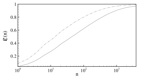
Figure 10: Energy sum ${\mathcal{E}}(n)=\sum_{j=1}^{n}E(j)$ for the Newtonian (solid lines) and for the visco-elastic (dashed lines) flow. The sums are computed in their respective energetic ordering. The Reynolds number is ${\rm Re}_{\tau}=125$.

One glaring difference between the two flows that stands out from Table 1 is the energy concentration in the few most dominant modes of the viscoelastic flow compared to the flat distribution of energy in the Newtonian flow. For example, the first, second and third dominant viscoelastic modes have all twice the energy of the corresponding first, second and third dominant Newtonian modes. The sum of the first four viscoelastic energies contain as much as as the first ten Newtonian modes. The first 15 viscoelastic modes already contain more than 50% of the energy, whereas one needs to collect as many as 80 Newtonian modes to reach the same fraction of the total energy. In Fig. 10 we display the sum ${\mathcal{E}}(n)=\sum_{j=1}^{n}E(j)$ as a function of $n$ for both flows, where the sum is computed in the respective energy ordering. We note that the difference between the two curves is established within the first ten modes; for larger values of $n$ the lines are almost parallel, indicating a similar energy distribution between the less dominant modes.

IV.3 The energy spectrum

An interesting and illuminating way to discuss the difference between the two flows is provided by the energy spectrum. It was proposed in 90Ge that the main difference between the spectra of the two flows should appear in the position of the dissipative scale that separates a spectral power-law from exponential decay. The increase of the dissipative scale was indeed observed in recent DNS of homogoneous isotropic turbulence in the FENE-P model 02ACBP . However, the present results indicate that important changes involve the energy containing scales.

In Fig. 11 the energy is plotted for the two flows as a function of $n$. The Newtonian case displays a spectral plateau for the most dominant modes which crosses over to a power law for $n_{{}_{\rm N}}\geq 8$. In the case of the viscoelastic flow the plateau is dramatically higher, but also the power law changes its slope. It appears that the whole spectral curve is tilted in favor of the energy containing modes and on the expense of the lower energy modes and the dissipative modes.

The difference between the power laws can be made clearer by comparing with what can be obtained from the Kolmogorov law for high $k$-vectors. For relatively large $k$ we can expect the flow to isotropize 99ALP ; 02LPT , and Fourier modes would again become “best”. In this asymptotic situation (neglecting intermittency corrections) the spectrum $E(k)$ is expected to be $E(k)\propto k^{-11/3}$. In an isotropic environment we also expect that $n$ is proportional to the volume of the sphere of radius $k$, i.e. $n\propto k^{3}$. Thus we can expect for large values of $n$

$$E_{n}\propto n^{-11/9}\ ,\quad n\text{~{}large}\ .$$ (39)

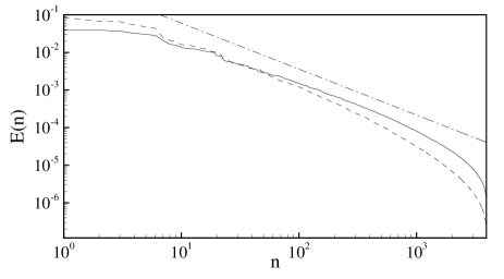
Figure 11: Log-log plots of the energy distribution $E_{n}$ vs mode index $n$ for the Newtonian case (solid line) and the viscoelastic case (dashed line). The rough K41 prediction (39) is shown by the dashed-dotted line. The Newtonian and visco-elastic dependencies are shown in their own energetic ordering. The Reynolds number is ${\rm Re}_{\tau}=125$.

The law proposed in Eq. (39) is displayed as the dashed-dotted line in Fig. 11. We see that it is in rough agreement with the power law section of the Newtonian spectrum, but it is certainly not in agreement with the viscoelastic spectrum which, as said before, is becoming steeper on the whole. This is a clear demonstration of the increase in energy of the energy containing modes on the expense of the others. We propose that even the power law section of the viscoelastic spectrum will not have a “universal” slope, but rather a slope that depends on the concentration of the polymer and the degree of drag reduction.

What emerges from this study is that understanding drag reduction lies in the reordering and energy redistribution of the energy containing modes. To examine these phenomena further we consider now the energy contents of the viscoelastic modes ordered by $n_{{}_{\rm N}}$ instead of their own ordering. This plot is a very vivid graphic representation of the data of Table 1, stressing very strongly the concentration of energy in the dominant viscoelastic modes, which are however rearranged in dominance compared to the Newtonian case.

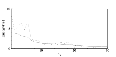
Figure 12: Plot of the energy content (in percentage of the total energy) for the Newtonian (solid line) and viscoelastic (dashed line) empirical modes. Both cases are plotted as a function of $n_{{}_{\rm N}}$.

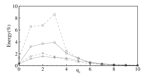
Figure 13: Energy of the most energetic modes for a given $\tilde{q}_{x}=0$ as a function of $\tilde{q}_{z}$. ${\rm p}=1$ modes are represented by circles and ${\rm p}=2$ modes by triangles. They are connected by solid lines for Newtonian modes, and by dashed line for viscoelastic modes.

Next we want to reiterate that one should focus on the most energetic modes. Noticing from Table 1 that all the dominant modes in both flows are associated with $\tilde{q}_{x}=0$, we consider next these modes as a function of $\tilde{q}_{z}$ for $p=1,2$. In Fig. 13 we show the energy of these modes. We note that the dramatic redistribution of energy occurs only for the most energetic modes with $p=1$; The less energetic modes are not affected much. Already the modes with $p=2$ are seen in the figure to be affected in a negligible way. In our opinion this is a clear message that to understand drag reduction we need to understand the rearrangement of the energy containing modes. For our flow configuration the most relevant are the modes which are space homogeneous in the spanwise direction. It should be stressed however that different geometries, and even channel geometry with different aspect ratios, may bring forth other modes as the most relevant ones. Nevertheless we expect that drag reduction would always be associated with a substantial increase in the energy containing modes, whatever these are for a given flow configuration.

V conclusions

In this paper we initiated a systematic study of drag reduction on the basis of DNS of the FENE-P model. We investigated simulations of Newtonian and viscoelastic flows in channel configuration at the same friction Reynolds number. Our main aim is to understand the mechanism of drag reduction. Since drag reduction involved modifications of the mean flow and of the large scale gradients in the flow, we are motivated to understand more the energy containing modes, rather than focusing only on phenomena of small scales. To this aim we have found first the list of empirical modes that represent the velocity field in an optimal way in an energy decreasing ordering. The first important discovery was that this list contains the very same modes for the Newtonian and viscoelastic flows. We propose that this finding will offer a huge simplification in any future theory of drag reduction. While we cannot offer a clean explanation of this finding, we can proceed at this time taking the approximate invariance of the modes as an empirical fact. What needs to be understood is just the energy distribution and reordering of the modes in the viscoelastic case.

We should stress that the point of view proposed here differs in a fundamental way from the approach presented for example in Refs. 69Lu ; 90Ge ; 01BFL . The thinking there focuses on the energy cascade in the turbulent flow, and on the modification of the small dissipative scales. Roughly speaking, the maximal gradients of the velocity are estimated from balancing the RHS of Eq. (4). Neglecting the statistical correlation between the conformation tensor and the velocity gradient, one can estimate the maximal velocity gradient by $\langle\partial u/\partial r\rangle\sim 1/\tau_{\rm p}$. Thus the matching of the polymer relaxation time with an eddy turn over time is used to predict a decrease in the maximal velocity gradient which is interpreted as drag reduction. We take an exception to this approach. First, a careful analysis of the space dependence of the conformation tensor shows that it is highly correlated with the velocity gradients (see for example 98DSB ; 02ACBP ; 02BP . Thus the estimate taken above is questionable at best. But moreover, we have shown that the main changes between the Newtonian and the viscoelastic modes occur in the energy containing modes. The energy containing modes are highly anisotropic, they are not Fourier modes, and their connection to the small scales where the isotropised Kolmogorov picture is tenable is very unclear. A theory that assumes a K41 spectrum down to a modified viscous scale does not appear tenable for the FENE-P flow, as seen in Fig. 11. We propose that a theory of drag reduction entails an understanding of the relative energy of the modes that characterize the largest scales of the flow.

To understand the relative ordering and the relative energy of the most dominant modes one needs to study the energy intake by these modes from the mean flow 01GLP ; 02GLP , the energy exchange between the modes, and the energy exchange with the viscoelastic subsystem represented by the conformation tensor field ${\bm{R}}({\bm{r}},t)$ 02ACBP ; 02BP . Such an investigation calls for measuring additional statistical objects like 3rd order correlation functions. The necessary simulation are in progress and the results will be published elsewhere.

- (1) K. R. Sreeinvasan and C. M. White, J. Fluid Mech. 409, 149 (2000).
- (2) J. L. Lumley, Ann. Rev. Fluid Mech. 1, 367 (1969).
- (3) P.S. Virk, AIChE J. 21, 625 (1975).
- (4) P.-G. de Gennes Introduction to Polymer Dynamics, (Cambridge, 1990).
- (5) J.M.J de Toonder, M.A. Hulsen, G.D.C. Kuiken and F.T.M Nieuwstadt, J. Fluid. Mech 337, 193 (1997).
- (6) C.D. Dimitropoulos, R. Sureshdumar and A.N. Beris, J. Non-Newtonian Fluid Mech. 79, 433 (1998).
- (7) E. de Angelis, C.M. Casciola and R. Piva, CFD Journal, 9, 1 (2000).
- (8) E. de Angelis, C.M. Casciola and R. Piva, Computers and Fluids, 31, 495 (2002).
- (9) R. Govindarajan, V.S. L vov and I. Procaccia, Phys. Rev. Lett., 87, 174501 (2001).
- (10) R. Govindarajan, V. S. L’vov and I. Procaccia, Stabilization of Hydrodynamic Flows by Small Viscosity Variations , Phys. Rev. E, submitted.
- (11) R.B. Bird, C.F. Curtiss, R.C. Armstrong and O. Hassager, Dynamics of Polymeric Fluids Vol.2 (Wiley, NY 1987).
- (12) A.N. Beris and B.J. Edwards, Thermodynamics of Flowing Systems with Internal Microstructure (Oxford University Press, NY 1994).
- (13) T.S. Luchik and W.G Tiederman, J.Fluid Mech. 190 241, 1987.
- (14) M. Kirby. L. Sirovich and M. Winter Phys. Fluids, 2 127 (1990).
- (15) K. Ball, L. Keefe and L. Sirovich, Int. J. for Numerical Methods in Fluids, 12, 585 (1991).
- (16) P.J. Holmes, J.L. Lumley, G. Berkooz, J.C. Mattingly and R.W. Wittenberg, Phys. Rep. 287, 337 (1997).
- (17) E. de Angelis, C.M. Casciola R. Benzi and R. Piva, Phys. Fluids, submitted.
- (18) E. Balkovsky, A. Fouxon V. Lebedev Phys. Rev. E, bf 64, 056301 (2001).
- (19) I. Arad, V. S. L’vov and I. Procaccia, Phys. Rev E59, 6753 (1999) .
- (20) V. S. L’vov, I. Procaccia and V. Tiberkevich, “Scaling Exponents in Anisotropic Hydrodynamic Turbulence”, Phys. Rev. E, in press.
- (21) R. Benzi and I. Procaccia, “A simple model for drag reduction” ,Phys. Rev. Lett., submitted. Also: cond-mat/0210523