Anomalous Diffusion in Infinite Horizon Billiards

Abstract

We consider the long time dependence for the moments of displacement $\langle|r|^{q}\rangle$ of infinite horizon billiards, given a bounded initial distribution of particles. For a variety of billiard models we find $\langle|r|^{q}\rangle\sim t^{\gamma_{q}}$ (up to factors of $\log t$). The time exponent, $\gamma_{q}$, is piecewise linear and equal to $q/2$ for $q<2$ and $q-1$ for $q>2$. We discuss the lack of dependence of this result on the initial distribution of particles and resolve apparent discrepancies between this time dependence and a prior result. The lack of dependence on initial distribution follows from a remarkable scaling result that we obtain for the time evolution of the distribution function of the angle of a particle’s velocity vector.

I Introduction

Diffusion of particles in an infinite domain billiard is a well studied problem [1-5,9,14]. By a billiard we refer to the motion of a point particle in a two dimensional domain in which the particle moves with constant velocity in straight line orbits executing specular reflection (i.e., angle of incidence equals angle of reflection) from fixed boundaries. By an infinite domain we refer to an unbounded two dimensional region. An early consideration of diffusion in a billiard as a model in physics was made by Lorentz [1] to model electrons in a metal. In this model (called the Lorentz gas) particles move freely and reflect specularly from fixed, randomly placed, hard-wall scatterers. A modification of the two dimensional Lorentz gas in which there are circular scatterers on a square lattice is an example of an infinite horizon billiard, called the Sinai billiard [5], and is illustrated in Fig. 1(a).

Figure 1: The four infinite horizon billiard structures that we consider include:(a) the Sinai billiard such that the channel width $W=L-2R>0$, (b) the Sinai billiard with random displacements $\Delta$ away from the square matrix such that $W=L-2(R+\Delta)>0$, (c) randomly oriented squares such that $W=L-\sqrt{2}d>0$, (d) scalloped channel with (d1) semicircular arcs and (d2) arcs subtending an angle less than $180^{o}$.

Infinite horizon billiards are the subset of infinite domain billiards that contain channels through which a particle may pass without ever reflecting off a billiard wall.

In this paper we consider diffusion in infinite horizon billiards. The examples that we study numerically are shown in Figs. 1(a)-(d). The billiards in Fig. 1 include: (a) the Sinai billiard, composed of circular, hard wall scatterers arranged on a square lattice such that the scatterers do not touch each other; (b) a modification of model (a) in which the circular scatterers are randomly displaced (random in direction and magnitude) by at most $\Delta<L/2-R$, so that there are channels of width $L-2(R+\Delta)$ accommodating free motion; (c) randomly oriented square scatterers on a square lattice; and (d) the scalloped channel, in which the domain is infinite in the $y$ direction and bounded in the $x$ direction by circular arc segments, each subtending an angle less than or equal to $180^{o}$. Figure 1(d1) shows the case of the scalloped channel where the circular arc segments are semi-circles, while Fig. 1(d2) shows the case where the arcs subtend an angle less than $180^{o}$. Particle motion for the situation in Fig. 1(d1) is equivalent to particle motion for a stadium-type billiard [see Fig. 2(a)]; the particle motion within the scalloped channel can be folded into the stadium billiard via reflection of the particle at a straight wall as it passes to the next cell.

Figure 2: (a)The stadium billiard has a domain bounded by two semi-circular arcs of radius $R$ and two straight lines of length $W$. Particle motion in this billiard can be mapped to motion in the scalloped channel [Fig. 1(d1)]. In a similar manner particle motion in the bounded domain billiard shown in (b) can be mapped to motion in the infinite domain billiard of Fig. 1(a).

By cells we mean each portion of the scalloped channel domain between the dotted lines of Fig. 1(d). In a similar manner particle motion in the bounded billiard of Fig. 2(b) can be thought of as equivalent to motion in the infinite billiard of Fig. 1(a).

One important means of characterizing transport in an infinite domain two dimensional billiard is through the phase space probability distribution function (pdf), $P(x,y,\theta,t)$, where $\theta$ is the angle of the particle velocity and we take all particle velocities to have magnitude one. From the pdf one can calculate the displacement moments of the distribution. The $q$th moment at time $t$ is

$$\langle r^{q}\rangle=\langle(x^{2}+y^{2})^{q/2}\rangle=\int_{0}^{2\pi}\int_{\mathcal{R}}(x^{2}+y^{2})^{q/2}P(x,y,\theta,t)\mathrm{d}{x}\mathrm{d}{y}\frac{\mathrm{d}\theta}{2\pi},$$ (1)

where $r=\sqrt{x^{2}+y^{2}}$ and $\mathcal{R}$ is the (infinite) spatial domain of the billiard and where throughout this paper we take the initial pdf, $P(x,y,\theta,0)$, to be bounded, $|P(x,y,\theta,0)|<K$, and to be zero outside some finite region. For the infinite horizon billiards shown in Fig. 1 we find that the moments of the displacement have a time dependence

$$\langle r^{q}\rangle\sim t^{\gamma_{q}},$$ (2)

which we use as shorthand for

$$\gamma_{q}=\lim_{t\to\infty}\frac{\log\langle r^{q}\rangle}{\log t}.$$ (3)

For all cases in Fig. 1 we find the exponent $\gamma_{q}$ to be

$$\gamma_{q}=\left\{\begin{array}[]{ll}q/2&q<2\\ q-1&q>2\end{array}\right..$$ (4)

Results of the form (2) with $\gamma_{q}$ composed of piecewise linear functions (different from (3)) have also been obtained in other situations of Hamiltonian transport [6, 7]. The occurrence of an exponent $\gamma_{q}\neq q/2$ is commonly referred to as anomalous diffusion, and $\gamma_{q}>q/2$ $(\gamma_{q}<q/2)$ is called superdiffusion (subdiffusion).

Figure 3: The dependence of the $q$th moment, $\langle|r|^{q}\rangle$, on time for the models discussed in this paper. Shown is the numerically determined time exponent $\gamma_{q}$; with the symbols $\times$, $\Box$, $*$, and + corresponding to the billiards depicted in Figs. 1(a), 1(b), 1(c), and 1(d1) respectively. The dashed line represents $\gamma_{q}=q/2$ and the dotted line represents $\gamma_{q}=q-1$.

Figure 3 shows the results of numerical experiments testing (4). In these numerical experiments we start with a cloud of many initial conditions distributed uniformly in the accessible space occupied by one cell [the region outside of the scatterer and within $0\leq y\leq L,0\leq x\leq L$ for Figs. 1(a)-(c), and $0\leq y\leq L$ for Figs. 1(d)] and uniformly in $0\leq\theta\leq 2\pi$. We then evolve the orbit of each particle in the cloud forward in time [8] and obtain $\langle r^{q}\rangle$. In all cases the results we obtain are consistent with (4). The motivation for choosing an initial distribution uniform in space and angle is that motion of an orbit from a typical initial condition in the billiards of Fig. 2 is known to be ergodic, generating an invariant density uniform in space and in angle $0\leq\theta\leq 2\pi$. In another set of numerical experiments we used initial conditions distributed uniformly in intervals of $\theta$ such that the lengths of the initial flights are bounded [e.g., for Figs. 1(a)-(c), $\theta_{0}\leq\theta\leq\pi/2-\theta_{0}$, $\pi/2+\theta_{0}\leq\theta\leq\pi-\theta_{0}$, $\pi+\theta_{0}\leq\theta\leq 3\pi/2-\theta_{0}$, $3\pi/2+\theta_{0}\leq\theta\leq 2\pi-\theta_{0}$ where $\theta_{0}<\pi/4$]. Again, agreement with (3) and (4) was found. This indicates that the angular particle distribution relaxes to the uniform distribution sufficiently fast that the results (3) and (4) are not modified. Explaining the reason for this insensitivity to the initial distribution is one of the main contributions of this paper (Sec. 2C). Our other main contribution is the result that, for long time, initial distributions with no particles in a $\theta$ interval about a direction of infinitely long flight (say $\theta=0$) lead to long-time distributions with an invariant scaling form. Specifically, $\hat{P}(\theta,t)=\int_{\mathcal{R}}P(x,y,\theta,t)\mathrm{d}x\mathrm{d}y$ approaches $\tilde{P}(\phi)$, where $\phi=\theta t$ and $\tilde{P}(\phi)$ is independent of $t$. Furthermore, the same $\tilde{P}(\phi)$ universally applies for the billiards of Figs. 1(a), 1(b), 1(c), 1(d2), but $\tilde{P}(\phi)$ is different for the billiard of Fig. 1(d1). We use this scaling result to show the insensitivity of (4) to the initial particle distribution.

Bleher [9] showed for infinite horizon billiards that the limit in distribution as $t\to\infty$ of the pdf of the particle displacements in the billiard is Gaussian with a width that increases with time as $\sqrt{t\log t}$. (For ordinary diffusion, the result is the same except that the width increases as $\sqrt{t}$.) However, the asymptotic $t$ dependence of the moments cannot be calculated from Bleher’s result. This is discussed in Sec. 3. Note that the definition of the symbol $\sim$ given in Eqs. (2) and (3) is such that logarithmic corrections to the scaling of $\langle r^{q}\rangle$ with time are not included [e.g., if $\langle r^{2}\rangle\cong Ct\log t$, where $C$ is a constant, as suggested by [9], then $\gamma_{2}$ from (3) is one, consistent with (4)].

II Theory

The difference between particle transport in an infinite horizon billiard and particle transport in the case of normal diffusion is due to the arbitrarily long trajectories found in the infinite horizon billiard. These long flights occur in the channels between the scattering boundaries of the billiard. When a particle is traveling nearly parallel to the axis of the channel [for Figs. 1(a)-(c) there are many channels parallel to both the $x$ and $y$ axes whereas for Fig. 1(d) there is only one channel, which is parallel to the $y$ axis], it will travel long distances between reflections off the billiard wall. Let $\theta_{n}$ be the angle between the trajectory of a particle and the axis of the channel after the $n$th reflection of that particle with a billiard wall. The length $r_{n}$ of the flight is of the order of $1/|\theta_{n}|$ for $|\theta_{n}|\ll 1$.

For some of the billiards we consider there are strong correlations between the $\theta$ values from one reflection to the next. This is especially true of the scalloped channel with semicircular arcs (stadium billiard). Here, upon reflection, the angle $\theta_{n}$ can change by, at most, a factor of three [12]; $|\theta_{n}|/3\leq|\theta_{n+1}|\leq 3|\theta_{n}|$. Thus if $|\theta_{n}|$ is small, $|\theta_{n+1}|$ is also small, and both represent long flights. This suggests an extreme model for the particle transport in which the length of a flight for each particle does not change from reflection to reflection; the length of each flight is completely correlated with the previous flight, but different particles have different flight lengths.

II.1 The Completely Correlated Model

Consider a one dimensional system in which an ensemble of particles executes a random walk. The particles in the ensemble differ from each other in the length of the step, $\Delta r_{\xi}$, each particle takes.

$$\Delta r_{\xi}=1/\xi,\ \xi\in[0,1].$$ (5)

The random variable $\xi$ is distributed uniformly in $[0,1]$ ($\xi$ is inspired by $\theta_{n}$ defined above, but is chosen to occupy the interval $[0,1]$ for simplicity), and $\xi$ for a particle does not change from step to step (complete correlation). Since every billiard particle has the same speed we normalize the magnitude of the velocity to 1 and thus take the time between steps in our one dimensional random walk model to be

$$\Delta t_{\xi}=1/\xi.$$ (6)

Since the random walk behaves like normal diffusion when the number of steps is large, the $q$th moment for each $\xi$, $\left\langle|r|^{q}\right\rangle_{\xi}$, will be

$$\langle|\frac{r}{\Delta r_{\xi}}|^{q}\rangle_{\xi}\sim(\frac{t}{\Delta t_{\xi}})^{q/2}\textrm{, for }t\gg\Delta t_{\xi}.$$ (7)

Substitution for $\Delta r_{\xi}$ and $\Delta t_{\xi}$ yields, for long time $t$, $(t\gg\Delta t_{\xi})$

$$\langle|r|^{q}\rangle_{\xi}\sim(t/\xi)^{q/2}$$ (8)

for each $\xi$.

To find the $q$th moment for the entire ensemble one needs to take an average over all particles:

$$\langle|r|^{q}\rangle=\int_{0}^{1}\langle|r|^{q}\rangle_{\xi}\mathrm{d}\xi.$$ (9)

This average has two main contributions:

$$\langle|r|^{q}\rangle\sim\int_{N/t}^{1}(t/\xi)^{q/2}\mathrm{d}\xi+\int_{0}^{1/t}t^{q}\mathrm{d}\xi$$ (10)

where $N$ is chosen to be large, so that the random walks have made many steps. The first term in Eq. (10) represents the fraction of particles that have executed at least $N$ steps and so can be described by Eq. (8). The second term comes from those particles that are still in their first flight (with velocity = 1). The contribution from the interval $N/t\geq\xi\geq 1/t$ [omitted in (10)] has neither the majority of walkers (in the limit of long time) nor the most extreme displacements and so does not dominate the other terms. For long time Eq. (10) yields

$$\langle|r|^{q}\rangle\sim\left\{\begin{array}[]{ll}t^{q/2}&q\leq 2\\ t^{q-1}&q\geq 2\end{array}\right..$$ (11)

This simple toy model shows that it is the very long flights allowed by the open channels that give rise to the non-Gaussian behavior for moments greater than 2. One might then think that for the real billiard systems of Fig. 1 the behavior for $q>2$ is a trivial result of the initial distribution of angles. However, this is not the case and the behavior (11) is robust to changes in the initial distribution of particles. As discussed in Sec. 2C, non-uniform initial angular distributions scatter rapidly enough that (11) still holds even if the initial distribution has no particles traveling nearly parallel to the channels.

II.2 Moment Equation for Infinite Horizon Billiards with a Uniform Initial Angular Distribution

We now consider a uniform initial spatial (within a cell) and angular distribution and for the case of the ergodic billiards of Figs. 1(a) (Sinai billiard) and 1(d) (scalloped billiard). In these cases such a distribution is stationary when $(x,y)$ is taken modulo the appropriate cell period. We show that $\gamma_{q}$ is given by Eq. (4) for these real billiard systems. The particle transport in an infinite horizon billiard must proceed at least as quickly as a random walk process (i.e., as fast as normal diffusion). While there exist mechanisms for faster than diffusive transport (to be discussed below), there is no stable mechanism to stop or trap a billiard particle. The periodic orbits that might trap the particle in these systems are all exponentially unstable. That a random walk is a lower bound on the transport in the billiard system implies that $\gamma_{q}\geq q/2$.

In addition to diffusive like behavior, particle trajectories that consist of a single long flight (“ballistic” flight) also participate in particle transport. If every particle were to move ballistically, we would find $\gamma_{q}=q$. This provides an upper bound on $\gamma_{q}$; not every particle will execute a single uninterrupted flight. We can, however, place a lower bound on the fraction of particle that do. Since the distribution of particle velocities is uniform in orientation, the fraction of particles executing flights of distance $vt$ or more (where $v$ is the velocity of the particle) involve a fraction of order of $W/t$ of the particles occupying a channel at any one time, where $W$ is the channel width defined in Fig. 1. (Although we have defined $v=1$, we retain $v$ in this section to clarify when we are speaking of distances and when we are speaking of times.) The contribution to $\langle|r|^{q}\rangle$ from these particles is

$$\langle|r|^{q}\rangle\gtrsim(vt)^{q}(C/t)=Ct^{q-1},$$ (12)

where $C$ is a constant depending on the size of the channel.

There are two points that can be fixed on the graph of $\gamma_{q}$ vs. $q$. The first is the zeroth moment, which by the conservation of probability is identically equal to one. Thus $\gamma_{0}=0$. The second point is fixed by the diffusion coefficient, which relates the second moment to time. It has been found [14] that $\langle r^{2}\rangle$ is of the order $t\log t$ and so, consistent with the definition (3), ignoring factors of $\log t$ we have $\gamma_{2}=1$.

Next we argue that $\gamma_{q}$ is a concave up function of $q$. Invoking the Cauchy-Schwartz inequality $(||(x\cdot y)||\leq||x||\times||y||)$, for $0\leq\epsilon\leq q$

$$\langle|r|^{q}\rangle=\langle|r|^{(q+\epsilon)/2}|r|^{(q-\epsilon)/2}\rangle\leq\langle|r|^{q+\epsilon}\rangle^{1/2}\langle|r|^{q-\epsilon}\rangle^{1/2}.$$ (13)

Thus

$$\log\langle|r|^{q}\rangle\leq\frac{\log\langle|r|^{q+\epsilon}\rangle+\log\langle|r|^{q-\epsilon}\rangle}{2}.$$ (14)

From (2), (3), and (14) we have that the graph of $\gamma_{q}$ versus $q$ is indeed concave up

$$\gamma_{q}\leq\frac{\gamma_{q+\epsilon}+\gamma_{q-\epsilon}}{2}.$$ (15)

Finally, we show that Eq. (4) holds, i.e., that $\gamma_{q}=q/2$ for $q\leq 2$ and $\gamma_{q}=q-1$ for $q\geq 2$. We have given lower bounds on $\gamma_{q}$, i.e. $\gamma_{q}\geq q/2$ and $\gamma_{q}\geq q-1$. We have also pinned the value of $\gamma_{q}$ at two values: $\gamma_{0}=0$ and $\gamma_{2}=1$. The first lower bound, the two known values of $\gamma_{q}$, and the concavity condition (15) force $\gamma_{q}=q/2$ for $q\leq 2$. There is a trivial upper bound on $\gamma_{q}$, $\gamma_{q}\leq q$. This upper bound, along with Eq. (14) implies that the slope of $\gamma_{q}$ never exceeds one. Since $\gamma_{2}=1$, $\gamma_{q}\leq q-1$ for $q\geq 2$. Therefore, for $q\geq 2$ both the upper bound and the lower bound coincide resulting in $\gamma_{q}=q-1$ for $q\geq 2$.

II.3 Non-uniform Initial Angular Distributions

The discussions of the previous two subsections relied on the existence of a uniform distribution for $\theta_{n}$ in the particle ensemble. This applies if one starts with a distribution uniform in angle and uniform in the space within a cell, in which case the particle ensemble will retain the uniform angular distribution. On the other hand, even if we have an initial distribution that is non-uniform, it will (under very general conditions) relax to the uniform distribution as time increases. The question we now address is whether this relaxation is fast enough to yield the same result for the temporal scaling of $\langle|r^{q}|\rangle$, Eq. (11), as the initially uniform distribution.

To consider this question, we first study the relaxation of an initial particle distribution with no particles in a finite gap around the channel direction. For example, for the scalloped channel we consider the case where the initial particle distribution is uniform in the space within a cell $\mathcal{C}$ and

$$P(x,y,\theta,t=0)=\left\{\begin{array}[]{ll}0&\textrm{for }|\theta|<\theta_{o}\textrm{ or }|\theta-\pi|<\theta_{o},\\ K&\textrm{ otherwise}\end{array}\right.,$$ (16)

where $0\leq\theta\leq 2\pi$ is the angle of the particle velocity vector with the $y$-axis, $K$ and $\theta_{o}$ are constants, and $(x,y)$ is in $\mathcal{C}$. Similarly, for the cases of Figs. 1(a)-1(c) we consider an initial distribution,

$$P(x,y,\theta,t=0)=\left\{\begin{array}[]{ll}0&\textrm{for }|\theta|,|\theta-\pi/2|,|\theta-\pi|,|\theta-3\pi/2|<\theta_{o},\\ K&\textrm{otherwise}\end{array}\right..$$ (17)

In particular, we focus on the behavior of $P(x,y,\theta,t)$ for $|\theta|$ small, $t$ large and $(x,y)$ in a channel. (Similar results apply for (17) with $|\theta-\pi/2|$ or $|\theta-\pi|$ or$|\theta-3\pi/2|$ small.) For all cases shown in Fig. 1, we find a remarkable scaling behavior. Let $\hat{P}(\theta,t)=\iint P\mathrm{d}x\mathrm{d}y$ where the spatial integral is over a channel. Then, if we introduce the scaled variable $\phi=\theta t$, we find that, in all the cases we have tested, the angular distribution function $\hat{P}(\theta,t)$ approaches a stationary form. That is,

$$\hat{P}(\theta,t)\to\tilde{P}(\phi)\textrm{ as }t\to\infty.$$ (18)

Figure 4: The time evolution of an initially uniform angular distribution of particles in the interval $[.3,\pi/2]$ for the scalloped channel with semi-circular arcs. The distribution is shown at three times; + at $t=27$, $\times$ at $81$, and $*$ at $243$. The distribution of particles in the channel of width $W$ becomes self-similar and static in the coordinate $\phi=\theta t$ with $\tilde{P}(\phi)=0$ for $\phi<\phi_{min}$.

We illustrate this with a numerical calculation on the scalloped billiard with $180^{o}$ arcs (Fig. 1(d1)) in Fig. 4. In generating this figure we follow the evolution of a large number of orbits initialized according to Eq. (16), and form the distribution $\hat{P}(\theta,t)$ using a histogram approximation. As shown, at successively larger $t$ the distribution approaches a time independent form $\tilde{P}(\phi)$ where $\tilde{P}(\phi)$ is zero for $\phi<\phi_{\textrm{min}}$, and, as $\phi$ increases past $\phi_{\textrm{min}}$, $\tilde{P}(\phi)$ increases, asymptoting to a constant for large $\phi$.

Figure 5: The time evolution of an initially uniform angular distribution of particles in the $\theta$ interval $[.3,\pi/2]$ for the Sinai billiard with $L/R=1$. The distribution is shown at four times; + at $t=9$, $\times$ at $27$, $*$ at $81$, and $\square$ at $243$. The distribution of particles in a channel becomes self-similar and static in the coordinate $\phi=\theta t$.

A similar numerical experiment for the Sinai billiard (Fig. 1(a)) yields the result in Fig. 5. In this case the large time distribution assumes the form,

$$\tilde{P}(\phi)=\left\{\begin{array}[]{ll}C(\phi/\phi_{o})&\textrm{ for }0<\phi<\phi_{o},\\ C&\textrm{ for }\phi>\phi_{o},\end{array}\right.,$$ (19)

where $C$ and $\phi_{o}$ are constants. Furthermore, we numerically obtain this same form for all the other cases of Fig. 1, [except for the case of the scalloped billiard with $180^{o}$ arcs (Fig. 1(d1)) which gives the result in Fig. 4]. We explain the reason for the result (19) and why it does not apply for the billiard of Fig. 1(d1) subsequently, but before doing that we first show that these results for $\tilde{P}(\phi)$ imply the applicability of Eq. (4) for the large time behavior of $\langle|r|^{q}\rangle$.

In order to show that (4) applies consider the fraction $\Xi(t_{o})$ of particles that, at some large time $t_{o}$, have $\phi<\phi_{*}$, where we take $\phi_{*}=2\phi_{\textrm{min}}$ for the case of Fig. 1(d1) and $\phi_{*}=\phi_{o}$ for the other cases. Noting that $\phi<\phi_{*}$ implies $\theta<\phi_{*}/t$, we have that for large $t_{o}$

$$\Xi(t_{o})\cong\int_{0}^{\phi_{*}/t_{o}}\tilde{P}(\theta t)\mathrm{d}\theta\\ =(t_{o})^{-1}\int_{0}^{\phi_{*}}\tilde{P}(\phi)\mathrm{d}\phi=Kt_{o}^{-1},$$ (20)

where $K$ is a constant. Between times $t_{o}$ and $2t_{o}$ these particles experience flights of length $\sim vt_{o}$. Hence for $t=2t_{o}$ these flights give a contribution to $\langle r^{q}\rangle$ that is approximately $(2K/t)(vt)^{q}\sim t^{q-1}$. Thus the lower bound (12) still applies, and, by the reasoning in Sec. 2B, we again obtain (4).

We note that the asymptotic time dependence $\tilde{P}(\phi)$ with $\phi\sim\theta t$ is marginal in the sense that, if the repopulation of an initially empty channel were slower (in the sense below), then (4) would not be recovered. In order to see this, consider the hypothetical case where an asymptotic distribution $P(\phi)$ of the form in Fig. 4 or Fig. 5 is still approached, but with a self-similar $\phi$ scaling given by $\phi_{\alpha}\sim\theta t^{\alpha}$. We have already considered the case $\alpha=1$, while $\alpha<1$ ($\alpha>1$) corresponds to slower (faster) filling in of the channel. If, for $0<\alpha<1$ (i.e. slow repopulation) we pursue the same reasoning as above for the $\alpha=1$ case, then we obtain the bound $\gamma_{q}\geq\alpha(q-1)$, and we can no longer conclude that (4) holds. For $\alpha>1$, we consider at time $t_{0}$ a range of angles $\theta_{+}\sim 1/t_{o}>\theta>\theta_{-}\sim\phi_{*}/t_{o}^{\alpha}$. Since $\alpha>1$, we have that $\theta_{+}\gg\theta_{-}$, and replacing $\theta_{-}$ by zero does not alter the estimate for the contribution to $\langle r^{q}\rangle$ from $\theta_{+}>\theta>\theta_{-}$. Thus the lower bound estimate of Sec. 2B still applies for $0<\alpha<1$.

We now discuss the asymptotic forms $\tilde{P}(\phi)$ illustrated in Fig. 4 for the scalloped billiard with $180^{o}$ arcs, and in Fig. 5 and Eq. (19) for the other cases.

First we discuss the scalloped billiard with $180^{o}$ arcs. A full treatment of the theory yielding $\tilde{P}(\phi)$ in this case will be given elsewhere [13]; in the present paper, we will limit our discussion to the basic reason for the difference between this case and the other cases. In particular, we discuss why, for this case, $\tilde{P}(\phi)=0$ in a finite interval about zero, $\phi<\phi_{\textrm{min}}$. From Fig. 1(d1) we see that after a long flight in the channel a particle will collide with the channel wall close to one of the cusp points where two arcs touch. For the case of $180^{o}$ arcs, the tangent to such a section of the channel wall is nearly horizontal. Thus, upon reflection $\hat{\theta}\equiv\textrm{min}(|\theta|,|\theta-\pi|)$ will still be small. In fact as shown in [12] by consideration of the geometry, $\hat{\theta}_{n+1}$ on the $(n+1)$st reflection cannot change by more than a factor of 3 from $\hat{\theta}_{n}$,

$$\hat{\theta}_{n}/3\leq\hat{\theta}_{n+1}\leq 3\hat{\theta}_{n},\textrm{ for }\hat{\theta}_{n}\ll 1.$$ (21)

Thus, if $\hat{\theta}_{n}$ is small, $\hat{\theta}_{n+1}$ is still relatively small. We can obtain the lower bound on $\phi$ by considering the most extreme case where $\hat{\theta}$ always decreases by 3 on every bounce,

$$\hat{\theta}_{n+1}=\frac{1}{3}\hat{\theta}_{n},$$ (22)

$$t_{n+1}=t_{n}+W/(v\hat{\theta}_{n}),$$ (23)

where $W$ is the channel width defined in Fig. 1(d1), $v$ is the particle velocity, and $t_{n}$ is the time of the $n$th reflection. Multiplying (22) by (23) we have

$$\hat{\phi}_{n+1}=\frac{1}{3}\hat{\phi}_{n}+W/v,$$ (24)

which, for large $n$, asymptotes to the solution $\hat{\phi}=3W/(2v)$. Thus $\phi_{\textrm{min}}=3W/(2v)$, which agrees with our numerical solution Fig. 4 (see also [13]).

In contrast to the case of the scalloped channel with $180^{o}$ arcs, in the other cases shown in Fig. 1, the scattering of a long flight upon reflection from a channel wall leads to a much more drastic change in the angle of a particle’s velocity vector with respect to the channel axis. For example, for the case of the Sinai billiard, the angular deflection is typically of order $\hat{\theta}^{1/2}$ which , for small $\hat{\theta}$, is much larger than $\hat{\theta}$. For the case of the scalloped channel with arcs of less than $180^{o}$, a particle moving nearly parallel to a channel axis is scattered by an angle of order one. Furthermore, after a large deflection, the orientation of the particle’s velocity vector is rapidly randomized by a succession of many reflections which, since the particle is no longer in a long flight, can occur in a relatively short time. These considerations lead us to a model for the cases in Figs. 1(a)-1(c) and 1(d2) in which we adopt the model hypothesis that, when a particle in a long flight suffers a collision with a billiard wall, the orientation of its velocity vector is randomly scattered with uniform probability density in $[0,2\pi]$. We wish to determine the evolution from the initial condition (a) in Fig. 6 for the case $\theta_{\textrm{max}}\ll 1$.

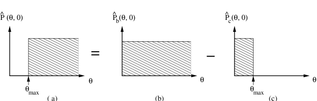
Figure 6: An initial distribution of particles with trajectories uniform in the angle $\theta$ for $\theta>\theta_{\textrm{max}}$ and zero for angles $\theta<\theta_{\textrm{max}}$, Fig. (a), is equivalent to a distribution uniform for all $\theta$, Fig. (b), minus a distribution that is uniform for $\theta<\theta_{\textrm{max}}$ and zero for $\theta>\theta_{\textrm{max}}$, Fig. (c). We use the time evolution of the distributions in Figs. (b) and (c) to find the time evolution of Fig. (a), see Fig. 7.

This initial distribution is equal to the initial distribution (b) in Fig. 6 minus the initial distribution (c) in Fig. 6. The initial condition (b), which is uniformly distributed in angle, remains unchanged when it is evolved forward in time $[\hat{P_{b}}(\theta,t)=\hat{P_{b}}(\theta,0)]$, since it is an invariant distribution. Thus, to find the evolution from initial condition (a), we can determine the evolution from (c), and then subtract it from (b). The long time evolution from (c) can be found by considering the time at which particles are scattered. Consider, for example, the scalloped channel, Fig. 1(d2), and a particle with a small initial $\theta_{o}$. Suppose the particle is located in the channel at a distance $\Delta x$ from the boundary of the channel with which it will collide [left or right vertical dashed line in Fig. 1(d2)]. If $\Delta x<vt\sin\theta_{o}\cong vt\theta_{o}$, the particle scatters; if $\Delta x>vt\theta_{o}$, it does not scatter. Since the particles we are considering are in the channel, $\Delta x<W$, every particle with $\theta_{o}>W/(vt)$ must have scattered at least once. We assume that $t>W/(v\theta_{max})\equiv t_{o}$. Since $\theta_{\textrm{max}}$ is small, the scattered particles contribute a small positive value of order $\theta_{\textrm{max}}$ to $\hat{P}_{c}(\theta,t)$ in $0\leq\theta\leq 2\pi$. Thus $\hat{P}_{c}(\theta,t)$ is small (i.e., of order $\theta_{\textrm{max}}$) for $\theta>W/vt$. For $\theta_{o}<\Delta x/(vt)$, $t>t_{o}$, the particle has not yet scattered. Assuming that the initial spatial distribution of particles in the channel is uniform, the fraction of particles with initial angle $\theta_{o}$ that have scattered is $\theta_{o}vt/W$. Thus

$$\hat{P}_{c}(\theta,t)\cong\left\{\begin{array}[]{ll}\hat{P}_{c}(\theta,0)(1-\theta vt/W)&\textrm{ for }\theta<W/(vt),\\ 0&\textrm{ for }\theta>W/(vt)\end{array}\right.,$$ (25)

where we have neglected the small, order $\theta_{max}$, contribution to $\hat{P}_{c}(\theta,t)$ from scattered particles. Subtracting $\hat{P}_{c}$ from $\hat{P}_{b}$ as illustrated in Fig. 7, we obtain the time asymptotic form in Fig. 5 and Eq. (19).

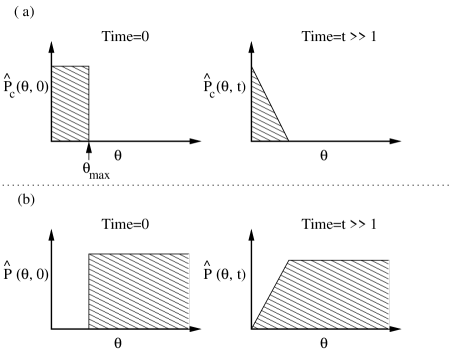
Figure 7: The evolution of $\hat{P}_{c}(\theta,t)$ and $\hat{P}(\theta,t)$.

III Discussion

As mentioned in the introduction, Bleher [9] proved, up to some natural conjectures that “For any periodic configuration of scatterers with an infinite horizon the limit in distribution

$$\lim_{t\to\infty}\frac{r(t)-r(0)}{(t\log t)^{1/2}}=\eta$$ (26)

exists and $\eta$ is a Gaussian random variable.” (We have substituted our $r(t)$ for Bleher’s $\mathbf{x}(t)$ for the sake of notational consistency).

We take no issue with Bleher’s proof referred to above, but we emphasize its use of limit in distribution convergence. This kind of convergence is the least restrictive kind of convergence considered within the context of probability and statistics. A proof of convergence in distribution implies only the ability to calculate the expectation value of functions that remain bounded. The convergence required by a limit in distribution is only strong enough to allow calculation of the expectations of functions that remain bounded [10]. Therefore the convergence of Bleher’s pdf is not strong enough to allow the moments of the distribution to be calculated. As a result of the strong weight $|r|^{q}$ puts on the tails of the distribution $(|r|\to\infty)$, two different distributions with the same limit in distribution can have very different moments.

The fact that Bleher is able to accurately (according to our simulations) calculate the second and lower moments of the displacement distribution suggests that his result can be strengthened to “convergence in $q^{th}$ mean” which is satisfied for a sequence $X_{n}$ if the expectation value of $|X_{n}-X|^{q}\to 0$ as $n\to\infty$. Convergence in $q^{th}$ mean also implies that the expectation value of $|X_{n}|^{p}$ limits to the expectation value of $|X|^{p}$ for $1\leq p\leq q$ [15]. Thus our results are consistent with convergence in $q$th mean to Bleher’s distribution for $q=2$, but rule out convergence for any higher value of $q$.

The inapplicability of Bleher’s result explains the discrepancy between Eqs. (2)-(4) and the result $\langle|r|^{q}\rangle\sim(t\log t)^{q/2}$ one would find by mistakenly calculating moments using Bleher’s pdf. Equations (2)-(4) also differ from normal diffusion, $\langle|r|^{q}\rangle\sim t^{q/2}$, as well as from the result suggested in [11].

In conclusion, our two main results are as follows:

(a) The moments $\langle r^{q}\rangle$ scale as $t^{\gamma_{q}}$ with $\gamma_{q}$ given by Eq. (4) for any initial bounded distribution,$|P(x,y,\theta,0)|<K$, that is zero outside some finite region (in particular, Eq. (4) still applies if the initial distribution has no particles with infinite flights).

(b) If the initial distribution has no particles in a $\theta-$interval about a direction of infinitely long flight (say $\theta=0$), then $\hat{P}(\theta,t)=\int_{\mathcal{R}}P(x,y,\theta,t)$ approaches a time-invariant scaling form $\tilde{P}(\phi)$, where $\phi=\theta t$ and $\tilde{P}(\phi)$ is universally the same (Fig. 5) for the billiards of Figs. 1(a),1(b), 1(c), 1(d2), but is different (Fig. 4) for the billiard of Fig. 1(d1).

This work was supported by the Office of Naval Research (Physics) and by the National Science Foundation (award DMS 0104087). We thank L. Bunimovich and J. R. Dorfman for discussion.

IV References

a. Department of Physics and Institute for Research in Electronics and Applied Physics.

b. Department of Mathematics and Institute for Physical Science and Technology.

c. Department of Electrical and Computer Engineering.

1. H. A. Lorentz, Proc. Amst. Acad. 7:438, 585, 604 (1905)

2. E. H. Hauge, Lecture Notes in Physics, Vol. 31, p. 337. (1974).

3. G. Gallavotti, Lecture Notes in Physics, Vol. 38, p 236 (1975).

4. Ya. G. Sinai, Funkts. Anal. Ego Prilozh. 13:46 (1979).

5. L. A. Bunimovich and Ya. G. Sinai, Commun. Math. Phys. 78:479 (1981).

6. P. Castiglione, A. Mazzino, P. Muratore-Ginanneschi, A. Vulpiani, Physica D 134:75 (1999).

7. R. Ferrari, A. J. Manfroi, W. R. Young, Physica D 154:111 (2001).

8. The numerical simulations of the four examples were carried out in a single cell, such as the cells shown in Fig. 2. The path of a particle in the infinite domain billiard is extracted by reflection of the particle trajectory at each straight wall of the cell. For infinite domain billiards with random displacements, the displacement from the center of the cell was altered every time the particle reflected from a straight wall (i.e. entered a new cell). For simplicity we altered the displacement even when the particle entered a previously visited cell; thus the simulation differs slightly from the fixed scatterer scenario, but the discrepancy affects only lower order terms. Likewise the orientation of the square was altered every time the particle reflected from a straight wall.

9. P. M. Bleher J. Stat. Phys. 66:315 (1992).

10. A. Papoulis, Probability, Random Variables, and Stochastic Process, 4th ed. (McGraw-Hill, 1994).

11. G.M. Zaslavsky and M. Edelman, Phys. Rev. E 56:5310 (1997).

12. K.C. Lee, Phys. Rev. Lett. 60:1991 (1988).

13. D. N. Armstead B. R. Hunt and E. Ott, to be published (2002).

14. P. Dahlqvist, J. Stat. Phys. 84:773 (1996).

15. P. Pollett MS308 Probability Theory web page,
http://www.maths.uq.edu.au/ pkp/teaching/ms308/summaries/conv/conv.html.