Diffusive Lorentz gases and multibaker maps
are compatible with irreversible thermodynamics

Abstract

We show that simple diffusive systems, such as the Lorentz gas and multibaker maps are perfectly compatible with the laws of irreversible thermodynamics, despite the fact that the moving particles, or their equivalents, in these models do not interact with each other, and that the dynamics takes place in low-dimensional phase spaces. The interaction of moving particles with scatterers provides the dynamical mechanism responsible for an approach to equilibrium, under appropriate conditions. This analysis provides a refutation of the criticisms expressed recently by Cohen and Rondoni [Physica A 306 (2002) 117-128].

I Introduction

For nearly one hundred years, the Lorentz gas has been investigated as a model of diffusive transport of light tracer particles among heavier particles [1, 2, 3, 4, 5]. On the collisional time scale of the fast tracer particles, the heavy particles can be treated immobile, which simplifies the dynamics. Due to this simplification, the Lorentz gas plays a privileged and important role in the development of transport and kinetic theories. In the last decades, several versions of the Lorentz gas model have been mathematically studied in detail and the existence of a well-defined diffusion coefficient has been proved rigorously under certain conditions [6, 7]. Moreover, the Einstein relation between the coefficients of electrical conductivity and diffusion has also been proved for a Gaussian thermostated Lorentz gas in the presence of an external field [8, 9].

Ten years ago, one of us introduced the multibaker map as a simple model of deterministic diffusion [10]. This map is constructed by simplifying the Birkhoff-Poincaré map of the hard-disk Lorentz gas. The multibaker map is a spatial extension of the baker map described by Arnold and Avez [11] and previously by Hopf [12] who also described a spatially extended baker-type model identical, in many respects, to the multibaker map. The advantage of the multibaker map for a study of deterministic diffusion is that, like the baker map, it is exactly solvable and can be used to test specific hypotheses in the context of kinetic and transport theories. Several versions of the multibaker map have been proposed and investigated as models of different transport processes [10, 14, 15, 16, 17, 18, 19, 20, 21, 22, 23, 24, 25, 26, 27].

Recently Cohen and Rondoni have written a series of papers [28, 29, 30] where, among other things, the physical relevance of the Lorentz gas and multibaker map in irreversible thermodynamics is challenged. Their main criticism is that the Lorentz gas and multibaker map “represent noninteracting particle systems” so that they “do not possess the crucial property of local thermodynamic equilibrium”. Hence “these models are not suited for a derivation of irreversible thermodynamics” (Ref. [29] p. 117) where, in their view, “the local physical density gradient $\partial n/\partial x$ acts like a real force which does work on the particles themselves”. In contrast, as claimed, “in the Lorentz slab there is no dissipation, no work done on the moving particles, hence no entropy production” (Ref. [29] p. 127).

Our purpose in this paper is to refute these criticisms. We show that the views of Cohen and Rondoni concerning both the status of the density gradient as a real force performing work on the particles and the physical unsoundness of the Lorentz gas and multibaker map from the point of view of irreversible thermodynamics, are wrong. Mátyás, Tél, and Vollmer have recently responded to criticisms of Cohen and Rondoni, directed at their work as well as ours, and expressed views along lines similar to those given here [31].

The plan of the paper is the following. In Section II, we give a brief review of the irreversible thermodynamics of diffusion in binary mixtures and clarify the status of the thermodynamic forces present. In the following Sections III and IV, we show that diffusion in the Lorentz gas and in the multibaker map is well described by, and compatible with irreversible thermodynamics, and that a local equilibrium indeed establishes itself in these systems.

II The irreversible thermodynamics of matter exchanges

In this section, we provide a first response to the claim that thermodynamic forces do work on the particles themselves and that this is a sine qua non condition for irreversible entropy production. We briefly review the irreversible thermodynamics of isothermal diffusion in multi-component mixtures and show how it applies to Lorentz gases, considered as binary mixtures of light and infinitely massive particles. Moreover, we show that the entropy production of diffusion does not vanish in binary mixtures of particles with an extreme mass ratio.

A The Second Law in the presence of matter exchanges

Classical irreversible thermodynamics is a local theory. It rests on the sole assumption that the densities of entropy $s$, internal energy $e$, and particle numbers $n_{k}$ are locally linked through a relation having the same structure as the relation linking the global analogs of these quantities in equilibrium:

$$s(\vec{r},t)=s\left[e(\vec{r},t),\{n_{k}(\vec{r},t)\}\right]\;.$$ (1)

The differentiable function $s$ has the same properties as the entropy

$$S=S(E,V,\{N_{k}\})=V\;s\left(\frac{E}{V},\left\{\frac{N_{k}}{V}\right\}\right)\;,$$ (2)

of a system at the internal energy $E$ and containing $N_{k}$ particles of substance $k$ in a volume $V$. Here, the identity of the two differentiable forms allows one to interpret the derivatives of $s$ with respect to $e$ and $n_{k}$ as being, respectively, the local reciprocal temperature and minus the chemical potential of substance $k$ multiplied by the reciprocal temperature.

Starting from Eq. (1) one can derive a balance equation of entropy by differentiating both sides with respect to time and by using the balance equations of mass, momentum, and energy of macroscopic physics. One obtains then in the balance equation a source term – the entropy production – in the form

$$\sigma_{\rm irr}=\sum_{\alpha}J^{(\alpha)}X^{(\alpha)}\geq 0\;,$$ (3)

where $J^{(\alpha)}$ is the thermodynamic flux associated with process $\alpha$ and $X^{(\alpha)}$ is the conjugate thermodynamic force. In a given system all these processes need not coexist. When they do they are, typically, coupled as long as certain symmetry requirements are satisfied.

The status of Eq. (1) from the standpoint of microscopic theory has been the subject of many investigations. Within the context of kinetic theory of gases, Prigogine [32] showed that a sufficient condition of validity is that the velocity distribution must remain close to the Maxwellian. This guarantees, at the same time, the validity of linear phenomenological relations linking the fluxes to the forces, a property that is less general than Eq. (3). However, Eq. (1) may still be correct under circumstances where the local equilibrium distribution is not a near-Maxwellian distribution in the energy [33]. The near-Maxwellization is sufficient for the validity of (1) but does not constitute a necessary condition. As a matter of fact, the main physics behind Eq. (1) is that after a short initial relaxation period the space-time variation of the probability distribution descriptive of the nonequilibrium system at hand can be expressed entirely in terms of the variation of the macroscopic (hydrodynamic) fields.

If a system exchanges matter $d{\cal N}_{k}$ as well as heat $dQ$ with its surroundings, the Second Law reads [34]

$$\Delta S=S_{\rm II}-S_{\rm I}\geq\int_{\rm I}^{\rm II}\left(\frac{dQ}{T}+\sum_{k}{\cal S}_{k}\;d{\cal N}_{k}\right)\;,$$ (4)

where $\Delta S$ is the total change of entropy in the system, not including the surroundings, ${\cal S}_{k}$ is the partial molar entropy of substance $k$, and ${\cal N}_{k}$ denotes the number of moles of this substance. In a closed system that does not exchange matter with its surrounding (i.e., $d{\cal N}_{k}=0$) but only heat, we recover the well-known inequality

$$\Delta S=S_{\rm II}-S_{\rm I}\geq\int_{\rm I}^{\rm II}\frac{dQ}{T}\;,$$ (5)

which implies that if no heat is transferred to a closed system, there may still be a transient irreversible increase of entropy. On the other hand, in an open system, matter exchange contributes to entropy production beside processes of heat exchange. In this regard, we mention that the study of processes of exchange of matter requires the consideration of chemiostats (particle reservoirs) instead of thermostats (heat reservoirs).

B Irreversible thermodynamics of diffusive processes in mixtures

Transport by diffusion is a process in which there is an exchange of matter from one macroscopic part of a system to another. This irreversible process can take place in a system in which no other irreversible process occurs. We then have a process where there is an exchange of matter contributing to entropy production without further contribution, for instance, due to temperature or macroscopic velocity gradients. Processes of exchange of matter are very common in chemical thermodynamics [35]. In particular, the process of mixing of two distinct chemical species is well known to contribute to entropy production. In such processes, spatial inhomogeneities of chemical concentrations exist across the system before the thermodynamic equilibrium is reached. The diffusion of tracer particles in a fluid of other particles is an example of such an irreversible process with exchange of matter.

A fluid composed of tracer particles moving among other particles can be considered as a binary mixture. It is well known that an isothermal $c$-component mixture at rest (i.e., with a zero macroscopic velocity field) can only sustain $(c-1)$ independent diffusive processes [34, 36]. In a binary mixture, we should thus expect a single diffusive process. It is a process of mutual diffusion between the tracer particles and the other particles. The position of the tracer particles is defined with respect to the center of mass of the total system.

The thermodynamics of a $c$-component mixture is based on the Gibbs relation

$$dE=T\;dS-P\;dV+\sum_{k=1}^{c}\;\mu_{k}\;dN_{k}\;,$$ (6)

where $T$ is the temperature, $P$ the pressure, and $\mu_{k}$ the chemical potential of particles $k$. If we define the densities of energy, entropy, and particles $k$ respectively as [cf. Eq. (2)]

$$e=\frac{E}{V},\qquad s=\frac{S}{V}\;,\qquad\mbox{and}\qquad n_{k}=\frac{N_{k}}{V}\;,$$ (7)

we obtain the local Gibbs relation [37]

$$de=T\;ds+\sum_{k=1}^{c}\mu_{k}\;dn_{k}\;.$$ (8)

The extensivity of the energy, entropy, and particle numbers together with the local Gibbs relation (8) imply the Gibbs-Duhem relation

$$s\;dT-dP+\sum_{k=1}^{c}n_{k}\;d\mu_{k}=0\;,$$ (9)

which shows that, for an isothermal and isobaric system ($dT=dP=0$), the variations of the chemical potentials are interconnected by

$$\sum_{k=1}^{c}n_{k}\;\vec{\nabla}\mu_{k}=0\;.$$ (10)

On the other hand, in absence of chemical reactions, local conservation of particles holds, yielding

$$\partial_{t}\;n_{k}+\vec{\nabla}\cdot\left(n_{k}\,\vec{u}+\vec{J}_{k}\right)=0\;,$$ (11)

where $\vec{J}_{k}$ is the current density of particles $k$ with respect to the local barycentric velocity $\vec{u}$ of the fluid, which is the velocity of the center of mass of a fluid element. The local conservation of the total mass implies that the currents are related by

$$\sum_{k=1}^{c}m_{k}\;\vec{J_{k}}=0\;,$$ (12)

where $m_{k}$ denotes the mass of one particle of component $k$.

As a consequence of the constraints (10) and (12) only $(c-1)$ gradients and currents are independent because

$$\vec{\nabla}\mu_{c} = -\sum_{k=1}^{c-1}\frac{n_{k}}{n_{c}}\;\vec{\nabla}\mu_{k}\;,$$ (13)

$$\vec{J}_{c} = -\sum_{k=1}^{c-1}\frac{m_{k}}{m_{c}}\;\vec{J}_{k}\;.$$ (14)

In an isothermal $c$-component mixture at rest ($\vec{u}=0$), the entropy production is therefore given by [36]

$$\sigma_{\rm irr}=\sum_{k=1}^{c}\vec{J}_{k}\cdot\left(-\vec{\nabla}\frac{\mu_{k}}{T}\right)=\sum_{k=1}^{c-1}\vec{J}_{k}\cdot\vec{X}_{k}\;,$$ (15)

with the thermodynamic forces

$$\vec{X}_{k}\equiv-\vec{\nabla}\frac{\mu_{k}}{T}-\sum_{l=1}^{c-1}\frac{m_{k}n_{l}}{m_{c}n_{c}}\;\vec{\nabla}\frac{\mu_{l}}{T}\;.$$ (16)

In a binary mixture ($c=2$), the entropy production contains only the contribution from the single diffusive process the system can sustain

$$(c=2)\qquad\qquad\sigma_{\rm irr}=-\left(1+\frac{m_{1}n_{1}}{m_{2}n_{2}}\right)\;\vec{J}_{1}\cdot\vec{\nabla}\frac{\mu_{1}}{T}\;.$$ (17)

If the tracer particles of mass $m_{1}$ are much lighter than the other particles of mass $m_{2}$ and, moreover, if the tracer particles are dilute

$$m_{1}\,n_{1}\ll m_{2}\,n_{2}\;,$$ (18)

the entropy production reduces to the simple expression

$$\sigma_{\rm irr}=-\vec{J}_{1}\cdot\vec{\nabla}\frac{\mu_{1}}{T}\;,$$ (19)

corresponding to the simple diffusion of the tracer particles. The heavy particles fix the center of mass with respect to which the transport is defined and they play the role of scatterers for the lighter particles. The thermodynamic flux of this diffusive process can thus be identified as the current of the tracer particles

$$\vec{J}^{\rm(D)}\equiv\vec{J}_{1}\;,$$ (20)

while the associated thermodynamic force is given in terms of the gradient of the chemical potential of the tracer particles as [38]

$$\vec{X}^{\rm(D)}=-\vec{\nabla}\frac{\mu_{1}}{T}\;.$$ (21)

Moreover, for dilute tracer particles, the chemical potential depends logarithmically on the tracer density $n_{1}$ according to

$$\frac{\mu_{1}}{T}=k_{\rm B}\;\ln\frac{n_{1}}{n_{1}^{0}}\;,$$ (22)

where $n_{1}^{0}$ is a reference density [35]. Hence, in a dilute system where the temperature, $T$, is constant, the thermodynamic force becomes

$$\vec{X}^{\rm(D)}=-k_{\rm B}\;\frac{\vec{\nabla}n_{1}}{n_{1}}\;,$$ (23)

which is independent of the temperature. The thermodynamic force is simply given in terms of the gradient of tracer density, and drives the irreversible process of matter exchange at the macroscopic level. This irreversible process occurs even if the tracer particles are so dilute that they never meet each other. The point is that the thermodynamic force of diffusion is a concept associated with a collection of particles, in contrast to the microscopic forces which directly act on the particles themselves. As we show in Sec. III A, such a force is indeed manifested as a Newtonian force at the level of momentum balance of the light particles but the type of balance one refers to here pertains to the average momentum taken over the probability distribution of the particles, as usual in fluid mechanics and in macroscopic physics in general. It may be worth recalling that in some molecular dynamics-inspired mechanisms of thermostating designed to sustain nonequilibrium steady states with shear or heat flow, the nonequilibrium constraint (an analog of the local thermodynamic force considered here) does modify the dynamics of the individual particles [39, 40]. In our view, this ingenious scheme, which stimulated many developments, is to be looked at as a prototypical model along with other thermostating mechanisms [41, 42, 43, 44, 45, 46]. In this connection we mention that nonequilibrium steady states with processes of matter exchange would require nonequilibrium constraints on particle numbers, that is, chemiostating mechanisms.

In the linear range of irreversible processes, the flux is proportional to the thermodynamic force. We shall write this proportionality in a form displaying Fick’s diffusion coefficient $\cal D$ rather than Onsager phenomenological coefficient,

$$\vec{J}^{\rm(D)}=-{\cal D}\;\vec{\nabla}n_{1}\;,$$ (24)

since $\cal D$ varies weakly in a wide range of values of $n_{1}$. Then the contribution of diffusion to the irreversible entropy production is given by

$$\sigma_{\rm irr}=\vec{J}^{\rm(D)}\cdot\vec{X}^{\rm(D)}=k_{\rm B}\;{\cal D}\;\frac{(\vec{\nabla}n_{1})^{2}}{n_{1}}\geq 0\;.$$ (25)

The diffusion coefficient $\cal D$ can be positive and finite even in the case of dilute tracer particles in a fluid. Since each tracer particle undergoes a random walk due to collisions with the surrounding fluid particles, a statistical collection of them appear to be driven from the regions where they are more concentrated toward the regions where their concentration is lower. The statistical character of the random walk is at the origin of the irreversible production of entropy. Thus, the absence of mutual interaction between the tracer particles does not prevent the existence of a thermodynamic force contributing to entropy production.

In conclusion, a careful application of the notion of thermodynamic force in the case of diffusion, as explained above, shows that the Cohen-Rondoni argument that, in the case of diffusion, the thermodynamic force should act on the particles themselves [29] is incorrect. It results from a failure to appreciate the fact that the thermodynamic force of diffusion has a statistical origin and should not be conceived as a microscopic force which acts on the particles themselves. Indeed, the tracer particles can be so dilute that they never come within interaction range among themselves although the thermodynamic force of diffusion is still non-vanishing and contributing to entropy production. Moreover, the derivation here above shows that the entropy production does not vanish in the Lorentz-gas limit $(m_{1}/m_{2})\to 0$ where the heavy particles are immobile.

In the next section, we show starting from a microscopic description that diffusion in the Lorentz gas is indeed well described by irreversible thermodynamics, and that the entropy produced corresponds to physical work that might be done on a moving piston, for example.

III The irreversible thermodynamics of the Lorentz gas

In this section, we show, contrary to the claims by Cohen and Rondoni [29], that the Lorentz gas can approach an equilibrium state through a local equilibrium and that a thermodynamic force as well as a friction force do exist in the Lorentz gas. Furthermore, we show that diffusion in the Lorentz gas yields a positive entropy production and that such an entropy production has a clear physical implication.

A $H$-theorem for the random Lorentz gas

The Lorentz gas model was introduced by Lorentz in 1905 as a model for transport of electrons in a solid [1]. It consists of a collection of fixed scatterers, and a collection of moving particles which do not interact with each other, but only with the fixed scatterers according to a well-defined potential energy function. Today, the Lorentz gas is often used as a model of diffusion of light particles among heavy ones [2, 3, 4, 5]. The heavy particles are immobile on the time scale of motion of the light particles, and the light particles are considered as not interacting with each other. At each elastic collision between light and heavy particles, energy is nearly conserved although momentum is not. Therefore, the randomization of the velocity direction is very fast albeit the randomization of energy occurs on a much longer time scale. This decoupling of time scales does not preclude the existence of a well-defined diffusion coefficient on each energy shell.

To set the stage we first analyze the transport properties and the thermodynamics of the Lorentz gas from the standpoint of kinetic theory. To this end we consider the random Lorentz gas with dilute scatterers, a version of the Lorentz model in which the diffusion coefficient has been evaluated some time ago using kinetic theoretic methods [2, 5]. More specifically, we consider a two-dimensional dilute random Lorentz gas. The scatterers are assumed to be hard disks of radius $a$ which are uniformly distributed on the plane with the density $n_{2}$. The motion of tracer particles is described by a linear Boltzmann equation, also known as the Boltzmann-Lorentz equation [2, 47]

$$\partial_{t}\;f+\vec{v}\cdot\vec{\nabla}f=\frac{n_{2}av}{2}\int_{-\pi}^{+\pi}d\varphi^{\prime}\left|\sin\frac{\varphi-\varphi^{\prime}}{2}\right|\left[f(\vec{r},\varphi^{\prime})-f(\vec{r},\varphi)\right]\;,$$ (26)

for the number density $f(\vec{r},\varphi)$ of tracer particles at position $\vec{r}$ with velocity angle $\varphi$, where $\vec{v}=v(\cos\varphi,\sin\varphi)$ is the velocity of the particles, $v$ their speed which is conserved as well as their kinetic energy $\epsilon=\frac{1}{2}m_{1}v^{2}$.

The Boltzmann-Lorentz equation (26) obeys a $H$-theorem based on the local entropy density

$$s(\vec{r})=k_{\rm B}\int_{-\pi}^{+\pi}d\varphi\;f(\vec{r},\varphi)\;\ln\frac{{\rm e}\;f^{0}}{f(\vec{r},\varphi)}\ ,$$ (27)

where $f^{0}$ is a constant, and ${\rm e}=2.718\ldots$ denotes the Naperian base. Indeed, the balance equation for this entropy density is given by

$$\partial_{t}\;s=-\vec{\nabla}\cdot\vec{J}_{s}+\sigma_{\rm irr}\;,$$ (28)

with the entropy current

$$\vec{J}_{s}=k_{\rm B}\int_{-\pi}^{+\pi}d\varphi\;\vec{v}\;f(\vec{r},\varphi)\;\ln\frac{f^{0}}{f(\vec{r},\varphi)}\ ,$$ (29)

and the local entropy production

$$\sigma_{\rm irr}=\frac{1}{4}\;k_{\rm B}\,n_{2}\,a\,v\int d\varphi\;d\varphi^{\prime}\;\left|\sin\frac{\varphi-\varphi^{\prime}}{2}\right|\left[f(\vec{r},\varphi^{\prime})-f(\vec{r},\varphi)\right]\;\ln\frac{f(\vec{r},\varphi^{\prime})}{f(\vec{r},\varphi)}\geq 0\ .$$ (30)

We emphasize that this $H$-theorem holds although all particles have the same energy $\epsilon=\frac{1}{2}m_{1}v^{2}$. The mechanism at the origin of this $H$-theorem is the randomization of the velocity angle, which establishes a local equilibrium in velocity direction. We notice that the existence of such a local equilibrium has already been pointed out by Lebowitz and Spohn in their work on heat conduction in the random Lorentz gas [48].

One can expand the density function as a Fourier series in the velocity angle $\varphi$ as

$$f=\sum_{k=-\infty}^{+\infty}f_{k}\;{\rm e}^{{\rm i}k\varphi}\;.$$ (31)

As a consequence of the Boltzmann-Lorentz equation (26) the Fourier components $f_{k}$ obey the following coupled differential equations

$$\partial_{t}\;f_{k}+v\;\frac{\partial_{x}-{\rm i}\partial_{y}}{2}\;f_{k-1}+v\;\frac{\partial_{x}+{\rm i}\partial_{y}}{2}\;f_{k+1}=\frac{8k^{2}}{1-4k^{2}}\,n_{2}\,a\,v\;f_{k}\;.$$ (32)

For particle distributions close to the microcanonical equilibrium, we keep only the first Fourier components so that

$$f(\vec{r},\varphi)\simeq\frac{1}{2\pi}\left[n_{1}(\vec{r})+\frac{2}{v^{2}}\;\vec{v}\cdot\vec{J}_{1}(\vec{r})\right]\ ,$$ (33)

where the density of tracer particles and their current are given by

$$n_{1}(\vec{r}) = \int_{-\pi}^{+\pi}f(\vec{r},\varphi)\;d\varphi\;,$$ (34)

$$\vec{J}_{1}(\vec{r}) = \int_{-\pi}^{+\pi}\vec{v}\;f(\vec{r},\varphi)\;d\varphi\;.$$ (35)

Substituting expansion (33) in the Boltzmann-Lorentz equation (26) and retaining the dominant terms, we get the balance equations for the number of tracer particles and for their current as

$$\partial_{t}\;n_{1} = -\vec{\nabla}\cdot\vec{J}_{1}\;,$$ (36)

$$\partial_{t}\;\vec{J}_{1} \simeq -\frac{8}{3}\,n_{2}\,a\,v\;\vec{J}_{1}-\frac{v^{2}}{2}\vec{\nabla}n_{1}\;.$$ (37)

Over a time scale longer than the relaxation time $\tau=\frac{3}{8n_{2}av}$, the current is driven by the gradient of density and we obtain from Eq. (37) Fick’s law on the energy shell as

$$\vec{J}_{1}\simeq-{\cal D}\;\vec{\nabla}n_{1}\;.$$ (38)

After substituting in Eq. (36) we obtain the diffusion equation

$$\partial_{t}n_{1}(\vec{r})={\cal D}\;\nabla^{2}n_{1}(\vec{r})\;,$$ (39)

with the energy-dependent diffusion coefficient

$${\cal D}=\frac{3\,v}{16\,a\,n_{2}}\;,$$ (40)

where $v=\sqrt{2\epsilon/m_{1}}$ is the speed of particles. Under these conditions, the entropy production (30) is straightforwardly shown to reduce to

$$\sigma_{\rm irr}\simeq k_{\rm B}\;\frac{\vec{J}_{1}^{2}}{{\cal D}\,n_{1}}\simeq k_{\rm B}\;{\cal D}\;\frac{(\vec{\nabla}n_{1})^{2}}{n_{1}}\geq 0\;,$$ (41)

which is the expression expected from irreversible thermodynamics, here shown to hold on a single energy shell.

We next show that the thermodynamic force of diffusion (23) appears explicitly in the balance equation for the momentum of the gas of tracer particles. We notice that the momentum density $\vec{g}_{1}$ of the tracer particles is directly proportional to the particle current $\vec{J}_{1}$ according to

$$\vec{g}_{1}\equiv m_{1}\;\vec{J}_{1}\;.$$ (42)

The balance equation (37) can thus be interpreted as the balance equation for the momentum of the gas of tracer particles. Moreover, we can introduce the partial mass density of the tracer particles as $\rho_{1}=m_{1}n_{1}$ and their drift velocity as

$$\vec{u}_{1}\equiv\frac{\vec{g}_{1}}{\rho_{1}}=\frac{\vec{J}_{1}}{n_{1}}\;.$$ (43)

This drift velocity can be considered as the velocity of an element of the gas of tracer particles. Since Eq. (37) gives the balance equation for momentum, we can now derive the time evolution of an element of the tracer gas as

$$\rho_{1}\;\frac{d\vec{u}_{1}}{dt}\simeq\underbrace{-\beta\;\rho_{1}\;\vec{u}_{1}}_{\vec{F}_{\rm friction}}\underbrace{-\epsilon\;\vec{\nabla}n_{1}}_{\vec{F}_{\rm thermo.}}$$ (44)

where we have neglected terms which are cubic in the gradients of the density. We notice that, to the order we keep, neglecting the cubic terms allows us to replace the partial time derivative in (37) by a total time derivative in (44). The constant $\beta=\frac{8}{3}n_{2}av$ is the friction coefficient, while $\epsilon$ is the kinetic energy of the particles. Eq. (44) can be interpreted as Newton’s equation for the element of the tracer gas. The left-hand side contains the mass of the gas element multiplied by its acceleration while the different Newtonian forces (per unit volume) acting on this gas element can be identified in the two terms of the right-hand side.

The first term is the Newtonian force of friction. The presence of this term contradicts the claim by Cohen and Rondoni that “fluxes of particles are moving frictionless” in the Lorentz gas (Ref. [29], p. 121). On the contrary, the infinitely heavy particles which are the scatterers produce a friction on the tracer gas because of the interaction of each tracer particle with the scatterers. We notice that conservation of total energy is here reduced to the property that the microscopic kinetic energy of the individual particles, $e=\epsilon\,n_{1}$, is locally conserved according to

$$\partial_{t}\;e+\vec{\nabla}\cdot(e\;\vec{u}_{1})=0\;.$$ (45)

Friction terms will be manifested when $e$ is decomposed into a macroscopic kinetic energy part, $n_{1}\vec{u}_{1}^{2}/2$, and an internal energy part. This is exactly along the same lines as the derivation of the balance equations of macroscopic physics.

The second term in the right-hand side of Eq. (44) involves the gradient of the density and can thus be identified as the Newtonian force driven by the thermodynamic force of diffusion (23). Indeed, we have a proportionality between both given by

$$\vec{F}_{\rm thermo.}=\frac{n_{1}\,\epsilon}{k_{\rm B}}\;\vec{X}^{\rm(D)}\;.$$ (46)

This result shows that, in the Lorentz gas, the thermodynamic force acts as a “real force” albeit on the statistical collection of particles which compose the gas element, even if the particles have no mutual interaction and, furthermore, conserve their energy during their whole motion. This is very similar to the role of pressure gradient in the momentum balance of a volume element of a fluid, which is present even in the limit of noninteracting particles. It is clear that this thermodynamic force does not act on the individual particles themselves. The concept of thermodynamic force applies to the statistical level of description but not to the microscopic one.

In the stationary state, the two terms in the right-hand side of Eq. (44) cancel, and one has

$$\vec{u}_{1}\simeq-\frac{\epsilon}{\beta\,\rho_{1}}\;\vec{\nabla}n_{1}\;.$$ (47)

The entropy production (41) of diffusion can then be expressed in terms of the dissipation arising from the friction

$$\sigma_{\rm irr}\simeq k_{\rm B}\;\frac{\beta\,\rho_{1}}{\epsilon}\;\vec{u}_{1}^{\,2}\;.$$ (48)

In Ref. [29], Cohen and Rondoni claim that there is no thermodynamic force for diffusion in the Lorentz gas, because there is no local equilibrium state described by a Maxwell-Boltzmann distribution with space and time dependent macroscopic quantities - the local density and temperature, and the local mean velocity. Here, we have demonstrated that despite its simplicity, the random Lorentz gas has all the ingredients needed for a description of its transport processes by irreversible thermodynamics. Thus the claims to the contrary by these authors appear to be mistaken. In our opinion they have not made a sufficiently careful distinction between the microscopic and macroscopic levels of description of the system, and they have not appreciated the fact that the approach to equilibrium in a Lorentz gas with a small density gradient also proceeds through a state of local equilibrium. Here the local equilibrium is not a state of near-Maxwellian velocity distribution but, rather, a state which is nearly uniform in the velocity direction, with a local density, even though all of the moving particles have the same energy. This local equilibrium is at the very origin of diffusion itself and, thus, of irreversible entropy production on each energy shell.

Finally, we notice that the random Lorentz gas is a useful model for the electronic conductivity at low temperature in a solid with impurities, and leads to a determination of the so-called residual resistivity. In this case, it is known that the conductivity is related to the diffusion coefficient and that both should be evaluated on the energy shell corresponding to the Fermi energy of the electron gas [49]. Diffusion as well as entropy production on a single energy shell have therefore experimental relevance.

B The periodic Lorentz gases as models of diffusion

We now proceed to the extension of the previous refutation of the criticisms by Cohen and Rondoni to the case of the periodic Lorentz gases where diffusion was rigorously proved. Using the methods of dynamical systems theory, which are free of the statistical hypotheses underlying kinetic theory, we show in the present subsection that, for these Lorentz gases, local equilibrium in the form discussed in Sec. III A and Fick’s law also hold on each energy shell and, in the following subsection, that this results in a positive entropy production.

In 1980, Bunimovich and Sinai proved that the two-dimensional hard-disk periodic Lorentz gas has a positive and finite diffusion coefficient if the horizon is finite, i.e., if no trajectory exists running through the lattice of hard disks without elastic collision [6]. A similar result has been proved by Knauf for the two-dimensional periodic Lorentz gas composed of scatterers with Yukawa potentials under the condition that the energy of the moving particle is large enough [7]. In addition, these Lorentz gases have been proved to be ergodic and mixing. The mixing property holds on each energy shell, and leads to the establishment of a local equilibrium in velocity direction. As in the case of the random Lorentz gas discussed above, this local equilibrium may be described by a spatial and velocity distribution which is nearly uniform in the directions of the velocity of the moving particles, and the spatial density varies only over distances large compared to the mean free path of the particles. This local equilibrium is sufficient for a transport by diffusion to occur, compatible with the laws of irreversible thermodynamics.

Mathematical proofs of the existence of diffusion in periodic Lorentz gases given by Bunimovich and Sinai and Knauf [6, 7], as well as extensions to higher orders in density gradients by Chernov and Dettmann [50], all imply the existence of a well behaved diffusion equation for these models. That is, on large spatial scales, compared to the mean free path of a particle, the diffusion occurs on each energy shell so that the density $f(\vec{r},\epsilon)$ of light particles with energy $\epsilon$ at position $\vec{r}$ obeys the diffusion equation

$$\partial_{t}\,f(\vec{r},\epsilon)\simeq{\cal D}(\epsilon)\ \nabla^{2}f(\vec{r},\epsilon)\;,$$ (49)

where ${\cal D}(\epsilon)$ is the diffusion coefficient on the shell of energy $\epsilon$, as proved in Ref. [6].

The diffusion equation (49) can be rewritten in the form of a local conservation law for the density $f(\vec{r},\epsilon)$ as

$$\partial_{t}\,f\ +\ \vec{\nabla}\cdot\vec{J}_{f}=0\;,$$ (50)

with the current

$$\vec{J}_{f}\simeq-{\cal D}(\epsilon)\;\vec{\nabla}f(\vec{r},\epsilon)\;.$$ (51)

This result, which was directly derived from the microscopic dynamics in Ref. [51], shows that Fick’s law holds on each energy shell in the Lorentz gas. This is a consequence of the property of local equilibrium in the velocity direction on each energy shell, and responds to the doubts expressed by Cohen and Rondoni [29] about the existence of a local equilibrium state and a corresponding Fick’s law in the periodic Lorentz gases.

At each elastic collision the energy $\epsilon$ of the particle is conserved so that the particle keeps its energy. Particles with different energies can thus be distinguished. Hence, the gas can be envisaged as a mixture of different gases with particles having different energies. These different gases ignore each other and each of them is the stage of an irreversible process of diffusion according to Eq. (49). In such a gas, the number of light particles per unit volume around the spatial point $\vec{r}$ is defined as

$$n_{1}(\vec{r})\equiv\int_{0}^{\infty}f(\vec{r},\epsilon)\;d\epsilon\;.$$ (52)

We can consider separately the gases of particles with different energies. If we remove from the system all the particles except those having their energy between $\epsilon$ and $\epsilon+\Delta\epsilon$ (with $\Delta\epsilon$ arbitrarily small), the particle density is given by

$$n_{1}(\vec{r})\simeq f(\vec{r},\epsilon)\;\Delta\epsilon\;.$$ (53)

As a consequence of the diffusion equation (49), the density (53) obeys the diffusion equation

$$\partial_{t}\,n_{1}(\vec{r})={\cal D}\;\nabla^{2}n_{1}(\vec{r})\;,$$ (54)

with the diffusion coefficient ${\cal D}={\cal D}(\epsilon)$. We notice that Eq. (54) as well as Eq. (49) are also found in the random Lorentz gas with the diffusion coefficient (40) according to the kinetic theory of the previous subsection.

The diffusion equation (54) describes processes in which the initial state is created by a spatial disturbance in the particle density $n_{1}$. Thereafter, the system relaxes back to a spatially uniform state according to Eq. (54). In this spatially uniform state, all the particles still have the same energy $\epsilon$ while their velocity angle is uniformly distributed in the interval $[0,2\pi[$ and their position is uniformly distributed in the whole space accessible to the particles. This uniform state is a microcanonical state for each one of the particles. This state plays the role of the state of thermodynamic equilibrium in the Lorentz gas.

C The thermodynamics of the Lorentz gas

Here, we show by using the methods of thermodynamics that diffusion in the Lorentz gases has a positive entropy production on each energy shell. We first establish the equilibrium thermodynamics of the Lorentz gas in the microcanonical ensemble and subsequently derive the balance equation for the entropy density in order to obtain the local entropy production.

The equilibrium thermodynamics of the hard-ball Lorentz gas is established as follows. Let us consider a gas of $N_{1}$ light particles without mutual interaction and moving in a spatial domain $\cal Q$ bounded internally by the hard balls and externally by a wall enclosing the Lorentz gas in a square, say. The volume of the domain $\cal Q$ is ${\cal V}={\rm Vol}({\cal Q})$. We notice that this volume is related to the physical volume $V$ by

$${\cal V}=V-N_{2}\;v_{2}\;,$$ (55)

where $N_{2}$ is the number of hard balls and $v_{2}$ is the volume of one hard ball. The phase space of this gas is

$${\cal M}=\left\{(\vec{r}_{1},\vec{p}_{1},...,\vec{r}_{N_{1}},\vec{p}_{N_{1}})|\vec{r}_{j}\in{\cal Q},\vec{p}_{j}\in\mbox{\mb R}^{d},x_{1}<x_{2}<\cdots<x_{N_{1}}\right\}\;,$$ (56)

where $\vec{r}_{j}=(x_{j},y_{j},z_{j})$ and the last conditions provide the ordering of indices required in the case of identical particles. The phase-space volume element is

$$dX=d\vec{r}_{1}\;\cdots\;d\vec{r}_{N_{1}}\;d\vec{p}_{1}\;\cdots\;d\vec{p}_{N_{1}}\;.$$ (57)

The system being ergodic, the equilibrium invariant distribution is given by a microcanonical distribution for a system of $N_{1}$ independent particles of kinetic energy between $\epsilon$ and $\epsilon+\Delta\epsilon$ (with $\Delta\epsilon$ arbitrarily small):

$$F(X)=\cases{\frac{\displaystyle N_{1}!}{\displaystyle{\cal V}^{N_{1}}}\;\left[\frac{\displaystyle\Gamma\left(\frac{d}{2}\right)\;\epsilon}{\displaystyle\left(2\pi m_{1}\epsilon\right)^{\frac{d}{2}}\;\Delta\epsilon}\right]^{\displaystyle N_{1}}\qquad{\rm for}\quad\displaystyle\epsilon<\frac{\vec{p}_{j}^{\,2}}{2m_{1}}<\epsilon+\Delta\epsilon\;,\cr\cr 0\qquad{\rm otherwise}\;,\cr}$$ (58)

which is normalized according to

$$\int_{\cal M}F(X)\;dX=1\;.$$ (59)

The entropy can be calculated as Gibbs’ coarse-grained entropy [52]

$$S=-k_{\rm B}\sum_{i}p_{i}\ln p_{i}\;,$$ (60)

by coarse graining the phase space into cells of size $\Delta X=\Delta^{N_{1}d}r\;\Delta^{N_{1}d}p=(\Delta r\Delta p)^{N_{1}d}$. This is the microscopic definition of the entropy which has been adopted in Refs. [54, 55] for nonequilibrium distribution. The probability for the system to belong to the $i^{\rm th}$ cell is

$$p_{i}=\int_{i^{\rm th}\;{\rm cell}}F\;dX\simeq F_{i}\;\Delta X\;,$$ (61)

so that

$$S\simeq k_{\rm B}\left\langle\ln\frac{1}{F(X)\;\Delta X}\right\rangle\;.$$ (62)

A straightforward calculation of the entropy (62) for the equilibrium distribution (58) leads to the formula

$$S\simeq k_{\rm B}\;N_{1}\;\ln\frac{{\cal V}\,{\rm e}\,(2\pi m_{1}\epsilon)^{\frac{d}{2}}\,\Delta\epsilon}{N_{1}\ \Gamma\left(\frac{d}{2}\right)\,\epsilon\,(\Delta r\Delta p)^{d}}\;,$$ (63)

in the limit $N_{1},{\cal V}\to\infty$, keeping the ratio $N_{1}/{\cal V}$ constant (where, again, ${\rm e}=2.718\ldots$ denotes the Naperian base). The energy of the gas is

$$E=N_{1}\;\epsilon\;.$$ (64)

We notice that $S$ is a well-defined differentiable function. As a consequence, differentiating both the formula (63) for entropy and the energy equation of state (64) with respect to the variables $V$, $N_{1}$, $N_{2}$, and $\epsilon$, we obtain the following identity which is known as the Gibbs relation [36]

$$dS=\frac{1}{\cal T}\;dE+\frac{P}{\cal T}\;dV-\frac{\mu_{1}}{\cal T}\;dN_{1}-\frac{\mu_{2}}{\cal T}\;dN_{2}\;,$$ (65)

with the inverse temperature

$$\frac{1}{\cal T}=\frac{d-2}{2}\;\frac{k_{\rm B}}{\epsilon}\ ,$$ (66)

the equation of state

$$\frac{P}{\cal T}=\frac{N_{1}\;k_{\rm B}}{V-N_{2}\,v_{2}}\;,$$ (67)

and the chemical potentials given by

$$\frac{\mu_{1}}{\cal T}=k_{\rm B}\;\ln\frac{N_{1}\;{\rm e}^{\frac{d}{2}-1}\;\Gamma\left(\frac{d}{2}\right)\,\epsilon\;(\Delta r\Delta p)^{d}}{(V-N_{2}\,v_{2})\,(2\pi m_{1}\epsilon)^{\frac{d}{2}}\,\Delta\epsilon}\;,$$ (68)

for the light particles and by

$$\frac{\mu_{2}}{\cal T}=\frac{N_{1}k_{\rm B}v_{2}}{V-N_{2}\,v_{2}}\;,$$ (69)

for the hard balls. It follows from Eqs. (68) and (69) that $\mu_{1}/{\cal T}$ and $\mu_{2}/{\cal T}$, which are related to the thermodynamic force of diffusion, are well defined. Notice that the inverse temperature happens to vanish in the two-dimensional case [cf. Eq. (66)], while the ratios of pressure and chemical potential to temperature are non-zero.

If we introduce the intensive quantities defined by Eq. (7), we obtain the other Gibbs relation

$$ds=\frac{1}{\cal T}\;de-\frac{\mu_{1}}{\cal T}\;dn_{1}-\frac{\mu_{2}}{\cal T}\;dn_{2}\;,$$ (70)

where the entropy density is given by

$$s=k_{\rm B}\;n_{1}\;\ln\frac{{\rm e}^{\frac{d}{2}}\;n_{1}^{0}}{n_{1}}\;,$$ (71)

with the reference density

$$n_{1}^{0}=\frac{(1-n_{2}v_{2})\,(2\pi m_{1}\epsilon)^{\frac{d}{2}}\,\Delta\epsilon}{{\rm e}^{\frac{d}{2}-1}\;\Gamma\left(\frac{d}{2}\right)\,\epsilon\,(\Delta r\Delta p)^{d}}\;.$$ (72)

In Eq. (70), the energy density is given by

$$e=n_{1}\;\epsilon\;,$$ (73)

the light-particle chemical potential by

$$\frac{\mu_{1}}{\cal T}=k_{\rm B}\;\ln\frac{n_{1}}{n_{1}^{0}}\;,$$ (74)

the hard-ball chemical potential by

$$\frac{\mu_{2}}{\cal T}=\frac{n_{1}k_{\rm B}v_{2}}{1-n_{2}\,v_{2}}\;,$$ (75)

and the inverse temperature by Eq. (66).

The relation (70) holds for the system at equilibrium. Its local equilibrium analog would amount to a supposition that the density $n_{1}$ of light particles presents small variations over large spatial scales while the energy $\epsilon$ and the hard-ball density $n_{2}$ remain constant, and the entropy density $s$ varies in such a way that the Gibbs relation (70) remains satisfied locally. The relaxation to such a state of local equilibrium finds its full justification in the complete ab initio derivation of entropy production given in Ref. [55]. The condition of validity is that the randomization of the velocity direction is faster than the relaxation of spatial inhomogeneities of the particle densities on each energy shell. The randomization time is given by the intercollisional time $\tau_{\rm coll.}\sim\ell/v$ which is estimated by the ratio of the mean free path $\ell$ to the speed $v=\sqrt{2\epsilon/m_{1}}$. The relaxation time is given by the diffusion time $t_{\rm diff.}\sim L^{2}/{\cal D}$ where $L$ is the wavelength characterizing the spatial inhomogeneities. Since ${\cal D}\sim v\ell$, the condition $t_{\rm diff.}\gg\tau_{\rm coll.}$ thus requires that the wavelength of the particle density is larger than the mean free path: $L\gg\ell$. This condition is independent of the speed so that it holds uniformly on all the energy shells.

For a nonequilibrium situation with a local variation of the density $n_{1}$ of light particles, we can now obtain the balance equation for the entropy density (71) on the basis of the knowledge that the particle density $n_{1}$ obeys the diffusion equation (54) in the Lorentz gas. The density $n_{2}$ of hard balls is constant in time and uniform in space. The entropy balance equation is obtained by taking the time derivative of the entropy density (71), replacing $\partial_{t}n_{1}$ by the right-hand side of Eq. (54), and splitting the result into a divergence term and a rest term which can then be identified as the local source of entropy, i.e. the irreversible entropy production. Performing this calculation yields the same balance equation as (28) but here with the entropy current

$$\vec{J}_{s}=-{\cal D}\;k_{\rm B}\;\left(\ln\frac{{\rm e}^{\frac{d}{2}-1}\,n_{1}^{0}}{n_{1}}\right)\;\vec{\nabla}n_{1}=-{\cal D}\;\vec{\nabla}s\;,$$ (76)

and the local irreversible entropy production

$$\sigma_{\rm irr}=k_{\rm B}\;{\cal D}\;\frac{(\vec{\nabla}n_{1})^{2}}{n_{1}}\geq 0\;,$$ (77)

which is always nonnegative by the Second Law of thermodynamics. The conclusion is here that the standard thermodynamic reasoning to derive entropy production [36] can be developed in the Lorentz gas and yields the same result as Eq. (41) obtained by kinetic theory in the case of the random Lorentz gas. The present derivation is more general in the sense that it also applies to the periodic Lorentz gas.

We now consider a gas of tracer particles moving in the same system as above, though with a nontrivial distribution of energy $f(\vec{r},\epsilon)$ obeying the diffusion equation (49). As mentioned above, such a gas can be considered as a mixture of different gases with particles having their energy defined within intervals $\Delta\epsilon$. The local entropy density of this gas is given by the sum of the local entropies (71)-(72) for the particles with different energies. Since the density of the particles of energy $\epsilon$ is given by $n_{1}(\vec{r})\simeq f(\vec{r},\epsilon)\Delta\epsilon$, we get the local entropy density of the whole gas as

$$s(\vec{r})=\int_{0}^{\infty}d\epsilon\;k_{\rm B}\;f(\vec{r},\epsilon)\;\ln\frac{(1-n_{2}v_{2})\,{\rm e}\,(2\pi m_{1}\epsilon)^{\frac{d}{2}}}{f(\vec{r},\epsilon)\ \Gamma\left(\frac{d}{2}\right)\,\epsilon\,(\Delta r\Delta p)^{d}}\;.$$ (78)

By performing a similar calculation as above but using the diffusion equation (49), we can obtain a balance equation similar to Eq. (28) now for the full entropy (78). In this case, the local irreversible entropy production in the Lorentz gas is given by

$$\sigma_{\rm irr}(\vec{r})=\int_{0}^{\infty}d\epsilon\;k_{\rm B}\;{\cal D}(\epsilon)\;\frac{\left[\vec{\nabla}f(\vec{r},\epsilon)\right]^{2}}{f(\vec{r},\epsilon)}\geq 0\;.$$ (79)

which is one of the central results of this paper. This result shows that the Lorentz gas with a distribution of energy can be considered as a mixture of different gases distinguished by the energy of their particles and that diffusion on each energy shell of the gas separately contributes to a positive entropy production. The main point is that, already in the microcanonical ensemble, the entropy production is positive with the typical form (77) expected from irreversible thermodynamics. The origin of this entropy production holds in the randomization of the velocity angle due to mixing in the Lorentz gas, which leads to the local equilibrium in the velocity direction.

In Refs. [17, 18, 53, 54, 55], it was shown that a similar calculation can be carried out ab initio at the microscopic level of description, which leads to the very same expression (77) that we have here derived using the local Gibbs relation (70) and the diffusion equation (49).

In conclusion, equations (41), (77) or (79) clearly demonstrate that entropy production does not vanish in the Lorentz gas, contrary to the claim by Cohen and Rondoni in Ref. [29] p. 127 that there is no entropy production in the Lorentz gas.

We notice that our result (79) applies not only to the Lorentz gas in which the mass ratio $m_{2}/m_{1}$ is infinite but also to a binary mixture where the mass ratio $m_{2}/m_{1}$ is large but finite. In this latter case, there still exists a mechanism which thermalizes and drives the velocity distribution toward the Maxwell-Boltzmann distribution even if this mechanism is slow. Under this assumption, the local distribution of energy can be supposed to be factorized into a local particle density $n_{1}(\vec{r})$ multiplied by a uniform equilibrium Boltzmann energy distribution of given temperature $T$ as

$$f(\vec{r},\epsilon)\simeq n_{1}(\vec{r})\;\frac{\eta(\epsilon)\,{\rm e}^{-\epsilon/k_{\rm B}{T}}}{\int_{0}^{\infty}\eta(\epsilon)\,{\rm e}^{-\epsilon/k_{\rm B}{T}}\;d\epsilon}\;,$$ (80)

where $\eta({\epsilon})$ is the density of states at energy $\epsilon$. Consequently, the local entropy density (78) takes the form

$$s(\vec{r})=k_{\rm B}\;n_{1}(\vec{r})\;\ln\frac{(1-n_{2}v_{2})\,{\rm e}^{\frac{d}{2}+1}\,(2\pi m_{1}k_{\rm B}{T})^{\frac{d}{2}}}{n_{1}(\vec{r})\;(\Delta r\Delta p)^{d}}\;.$$ (81)

expected from the Sackur-Tetrode formula where $\Delta r\,\Delta p=2\pi\hbar$ [56]. This result shows that our definition of entropy corresponds to the well-known physical entropy. Moreover, the entropy production (79) reduces to the form

$$\sigma_{\rm irr}\simeq k_{\rm B}\;\bar{\cal D}\;\frac{(\vec{\nabla}n_{1})^{2}}{n_{1}}\geq 0\;,$$ (82)

with the mean diffusion coefficient

$$\bar{\cal D}=\frac{\int_{0}^{\infty}\eta({\epsilon})\,{\rm e}^{-\epsilon/k_{\rm B}{T}}{\cal D}(\epsilon)\;d\epsilon}{\int_{0}^{\infty}\eta(\epsilon)\,{\rm e}^{-\epsilon/k_{\rm B}{T}}\;d\epsilon}\;.$$ (83)

With the assumption (80), Eqs. (82) and (83) thus give the values of entropy production and diffusion coefficient for the diffusion of light tracer particles in a dilute binary mixture at the temperature $T$, as can be derived from the results by Chapman and Cowling in Ref. [4]. We can therefore conclude that our whole calculation is consistent with common knowledge on irreversible thermodynamics and the kinetic theory of binary mixtures of light and heavy particles.

D Thermodynamic equivalence with a process producing work

We have already shown with Eqs. (44) and (46) that, in the random Lorentz gas, the thermodynamic force appears as a Newtonian force acting on statistical collections of particles. In the present subsection, our aim is to give a general argument demonstrating that the entropy production of diffusion in the Lorentz gases has a physical meaning, since it can be associated with the performance of work. We respond in this way to the doubts expressed by Cohen and Rondoni about a possible “confusion between information theoretic and real entropy” (Ref. [29] p. 118), and the allusion that entropy production in the Lorentz gas could only refer to an abstract information theoretic concept without physical consequence (Ref. [29] p. 118 & 128).

Let us consider a slab of the Lorentz gas of width $l$ between two large cubic reservoirs of the same volume $V=L^{d}$ containing respectively $N_{\rm L}$ and $N_{\rm R}$ light particles so that the particle densities in the reservoirs are respectively $n_{\rm L}=N_{\rm L}/V$, and $n_{\rm R}=N_{\rm R}/V$ (The subscript ‘L’ refers to the left-hand side and ‘R’ to the right-hand side, see Fig. 1). We here assume that the velocity distribution of the particles is initially taken to be a Maxwell-Boltzmann distribution at the same temperature $T$ across the whole system, i.e., the distribution function has the form (80) at the initial time with $n_{1}(\vec{r})$ taking the constant values $n_{\rm L}$ and $n_{\rm R}$ in the reservoirs and a linear interpolating profile inbetween. Since the diffusion process conserves the energy of each particle, the temperature, $T$, at the beginning is equal to the temperature after equilibrium is reached and there is no heat produced. However, there is a current of particles $J^{\rm(D)}$ from the high-density reservoir to the low-density one because of the difference of concentrations across the Lorentz slab. The current of particles decreases the difference of densities between both reservoirs. As long as there is a difference of densities, the system is out of equilibrium, and thermodynamic equilibrium is reached when $n_{\rm L}(t=\infty)=n_{\rm R}(t=\infty)=n_{\rm eq}=(N_{\rm L}+N_{\rm R})/(2V)$, and the current vanishes.

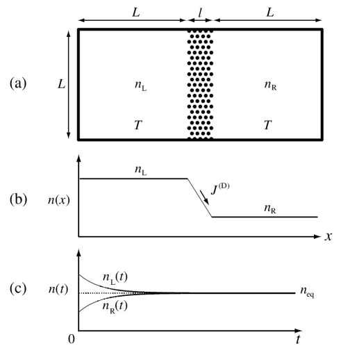
FIG. 1.: Irreversible process of diffusion across a Lorentz slab leading to the equilibration of densities between both reservoirs: (a) configuration of the system; (b) initial density profile across the system; (c) time evolution of the densities which decay to their equilibrium value in each reservoir.

The irreversible process of equilibration by the diffusion of particles across the Lorentz slab leads to a global production of entropy. Indeed, in the initial situation, the entropy of the whole system is equal to the entropies of the ideal gases in both reservoirs if the Lorentz slab is taken to be much smaller than the reservoirs ($l\ll L$) so that its entropy is negligible:

$$S_{\rm initial}=S_{\rm L}+S_{\rm R}\;,\qquad\mbox{with}\quad S_{\rm L}=k_{\rm B}N_{\rm L}\ln\frac{V\gamma}{N_{\rm L}}\;,\quad\mbox{and}\quad S_{\rm R}=k_{\rm B}N_{\rm R}\ln\frac{V\gamma}{N_{\rm R}}\;,$$ (84)

with the constant

$$\gamma=\frac{{\rm e}^{\frac{d}{2}+1}(2\pi m_{1}k_{\rm B}T)^{\frac{d}{2}}}{(2\pi\hbar)^{d}}$$ (85)

according to the Sackur-Tetrode formula [56]. The entropy after equilibration is given by

$$S_{\rm final}=k_{\rm B}(N_{\rm L}+N_{\rm R})\ln\frac{2V\gamma}{N_{\rm L}+N_{\rm R}}\;,$$ (86)

so that the total entropy increase is

$$\Delta S=S_{\rm final}-S_{\rm initial} = k_{\rm B}N_{\rm L}\ln\frac{2N_{\rm L}}{N_{\rm L}+N_{\rm R}}+k_{\rm B}N_{\rm R}\ln\frac{2N_{\rm R}}{N_{\rm L}+N_{\rm R}}$$ (87)

$$\geq k_{\rm B}N_{\rm L}\left(1-\frac{N_{\rm L}+N_{\rm R}}{2N_{\rm L}}\right)+k_{\rm B}N_{\rm R}\left(1-\frac{N_{\rm L}+N_{\rm R}}{2N_{\rm R}}\right)=0\;,$$ (88)

because of the inequality $\ln(1/x)\geq 1-x$. Accordingly, the entropy increase (87), which can be rewritten in the form

$$\Delta S=k_{\rm B}N_{\rm L}\ln\frac{n_{\rm L}}{n_{\rm eq}}+k_{\rm B}N_{\rm R}\ln\frac{n_{\rm R}}{n_{\rm eq}}\geq 0\;,$$ (89)

is positive in the above process without heat production.

We have now to show that the entropy increase (89) is irreversibly produced by diffusion in the Lorentz slab. Within the slab, the space and energy distributions $f(\vec{r},\epsilon)$ of the tracer particles evolve in time according to the diffusion equation (49). Since the reservoirs are much larger than the Lorentz slab ($L\gg l$) the diffusion process is quasi-stationary and a linear profile of density $f(\vec{r},\epsilon)$ is maintained in the slab during the whole relaxation to the equilibrium and, this, on each energy shell. The current (51) of particles of energy $\epsilon$ is thus transverse to the slab and equal to

$$J_{f}=-{\cal D}\;\frac{f_{\rm R}-f_{\rm L}}{l}\;,$$ (90)

where $f_{\rm R}$ and $f_{\rm L}$ are the densities of particles of energy $\epsilon$ in the reservoirs and ${\cal D}={\cal D}(\epsilon)$. These densities relax to their equilibrium values according to the equations

$$\frac{df_{\rm L}}{dt}=-\frac{df_{\rm R}}{dt}=-\frac{J_{f}}{L}\;.$$ (91)

The entropy of the total system is the sum of the entropies of both reservoirs plus the negligible entropy of the Lorentz slab. This total entropy can be expressed in terms of the entropy density $s$ which obeys the balance equation (28) so that the time derivative of the total entropy is given by

$$\frac{dS}{dt}=A\int dx\;\partial_{t}\,s=A\int dx\;(-\partial_{x}J_{s}+\sigma_{\rm irr})\;,$$ (92)

where $A=L^{d-1}$ is the area of a section of both reservoirs perpendicular to the direction of the current (see Fig. 1). The entropy production vanishes in both reservoirs and takes the positive value (79) in the Lorentz slab. Since the total system is isolated, the entropy current vanishes at its borders so that the only contribution to the entropy variation comes from the irreversible entropy production (79) in the Lorentz slab:

$$\frac{dS}{dt}=A\int dx\;\sigma_{\rm irr}=A\int_{L}^{L+l}dx\int_{0}^{\infty}d\epsilon\;k_{\rm B}\;{\cal D}\;\frac{(\partial_{x}f)^{2}}{f}\geq 0\;.$$ (93)

In a quasi-stationary evolution, the density of particles of energy $\epsilon$ is linear in the slab

$$f=f_{\rm L}+\frac{f_{\rm R}-f_{\rm L}}{l}\,(x-L)\;,\qquad\mbox{for}\quad L<x<L+l\;,$$ (94)

so that the entropy variation (93) becomes

$$\frac{dS}{dt}=k_{\rm B}\,A\int_{0}^{\infty}d\epsilon\;{\cal D}\;\frac{f_{\rm R}-f_{\rm L}}{l}\;\ln\frac{f_{\rm R}}{f_{\rm L}}\geq 0\;.$$ (95)

According to Eq. (90), the gradient of densities can be expressed in terms of the current whereupon

$$\frac{dS}{dt}=-k_{\rm B}\,A\int_{0}^{\infty}d\epsilon\;J_{f}\,\ln\frac{f_{\rm R}}{f_{\rm L}}\;.$$ (96)

Besides, Eq. (91) allows us to write the current as the time derivatives of the densities and we get

$$\frac{dS}{dt}=-k_{\rm B}V\int_{0}^{\infty}d\epsilon\left(\frac{df_{\rm L}}{dt}\;\ln f_{\rm L}+\frac{df_{\rm R}}{dt}\;\ln f_{\rm R}\right)\;,$$ (97)

where $V=AL$ is the volume of each reservoir. Eq. (97) can now be integrated over time to obtain

$$\Delta S=S_{\rm final}-S_{\rm initial}=k_{\rm B}V\int_{0}^{\infty}d\epsilon\left(f_{\rm L}\;\ln\frac{2\,f_{\rm L}}{f_{\rm L}+f_{\rm R}}+f_{\rm R}\;\ln\frac{2\,f_{\rm R}}{f_{\rm L}+f_{\rm R}}\right)\geq 0\;,$$ (98)

where $f_{\rm L}$ and $f_{\rm R}$ denote the initial distributions given by the Boltzmann distribution (80) with the initial densities $n_{\rm L}=N_{\rm L}/V$ and $n_{\rm R}=N_{\rm R}/V$, while the final distributions are equal to $(f_{\rm L}+f_{\rm R})/2$ in both reservoirs. The integral over the energy can be performed in Eq. (98) in the same way as the Sackur-Tetrode entropy (81) was obtained. Consequently, we recover the entropy increase (89) demonstrating that this entropy is irreversibly produced by diffusion in the Lorentz slab.

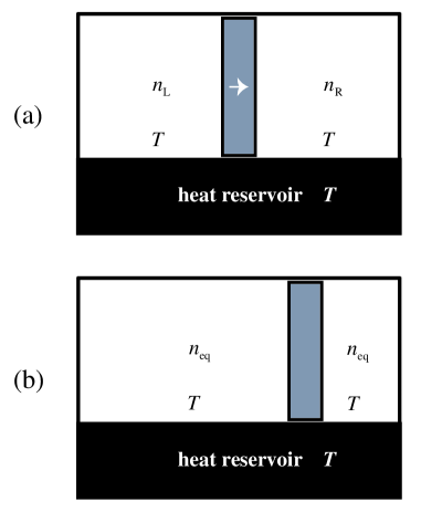
FIG. 2.: Replacement of the Lorentz slab by a movable piston so that work can be extracted from the difference of densities if the whole system is in contact with a heat reservoir: (a) initial configuration of the system; (b) final configuration after the work $W$ has been extracted.

Now, the entropy increase (89) corresponds to some work which could otherwise be used if we were to replace the Lorentz slab by a movable piston of equal volume, and if the system were put in contact with a heat reservoir (see Fig. 2). In the initial situation where there is a difference of particle densities between both sides, the piston is submitted to a force due to the difference of pressures

$$P_{{\rm L},{\rm initial}}=\frac{N_{\rm L}k_{\rm B}T}{V}\;,\qquad\mbox{and}\qquad P_{{\rm R},{\rm initial}}=\frac{N_{\rm R}k_{\rm B}T}{V}\;.$$ (99)

This force can produce work if the piston is slowly moved until both pressures equilibrate. We suppose that the piston is moved so slowly that the process is isothermal. The equilibrium of pressures is reached when the high-density, high-pressure fluid has expanded and compressed the fluid on the other side so that both have the same equilibrium density $n_{\rm eq}$, the temperature $T$ being kept constant. The volumes of both fluids have changed so that

$$n_{\rm eq}=\frac{N_{\rm L}}{V_{\rm L}}=\frac{N_{\rm R}}{V_{\rm R}}=\frac{N_{\rm L}+N_{\rm R}}{2V}\;,\qquad\mbox{and}\qquad P_{{\rm L},{\rm final}}=\frac{N_{\rm L}k_{\rm B}T}{V_{\rm L}}=P_{{\rm R},{\rm final}}=\frac{N_{\rm R}k_{\rm B}T}{V_{\rm R}}\;,$$ (100)

with $V_{\rm L}+V_{\rm R}=2V$, the numbers of particles being here constant in each fluid. The work extracted in this process is

$$W=\int_{\rm initial}^{\rm final}\left(P_{\rm L}\;dV_{\rm L}+P_{\rm R}\;dV_{\rm R}\right)=k_{\rm B}T\left(N_{\rm L}\ln\frac{V_{\rm L}}{V}+N_{\rm R}\ln\frac{V_{\rm R}}{V}\right)\;.$$ (101)

Since the ratios of volumes are equal to the ratios of densities

$$\frac{V_{\rm L}}{V}=\frac{n_{\rm L}}{n_{\rm eq}}\;,\qquad\mbox{and}\qquad\frac{V_{\rm R}}{V}=\frac{n_{\rm R}}{n_{\rm eq}}\;,$$ (102)

we find that the extracted work is equal to the temperature multiplied by the entropy increase during the previous process:

$$W=k_{\rm B}T\left(N_{\rm L}\ln\frac{n_{\rm L}}{n_{\rm eq}}+N_{\rm R}\ln\frac{n_{\rm R}}{n_{\rm eq}}\right)=T\;\Delta S\;.$$ (103)

Since the initial and final energies of the particles in both fluids are equal by the equation of state $E=(d/2)Nk_{\rm B}T$ for ideal gases, the work $W$ has been pumped from the heat reservoir. Accordingly, we conclude that the entropy (89) irreversibly produced by diffusion in the Lorentz slab corresponds to some work which is lost during the process of diffusion. In this sense, merely by randomizing the velocity directions of the particles, the diffusion process dissipates an energy which could otherwise be used, which confirms that diffusion in the Lorentz gas is an irreversible process obeying the Second Law of thermodynamics.

IV The irreversible thermodynamics of the multibaker model of diffusion

In this section, we show that the previous considerations for the diffusive Lorentz gas extend to the multibaker model of diffusion as well, contrary to the statement by Cohen and Rondoni that “there is no multibaker-analog of the concept of local thermodynamic equilibrium” (Ref. [29], p. 125).

A The multibaker map as a model of diffusion

The multibaker model can be considered to be a simplification of the Birkhoff map of the hard-disk Lorentz gas. The Birkhoff map of the Lorentz gas is the map induced by the collisional dynamics between the disk scatterers at constant energy. This map is constructed in terms of two Birkhoff coordinates: (i) the angle $0\leq\theta<2\pi$ of the position of collision on the disk, and (ii) the canonically conjugate variable which is the component $-1<\varpi=\sin\psi<+1$ of velocity that is tangent to the disk, $\psi$ being the angle between the velocity and the normal to the disk at collision. The kinetic energy $\epsilon$ is conserved during the whole motion so that the trajectories at different energies are similar after a rescaling of the time in terms of the speed $v(\epsilon)=\sqrt{2\epsilon/m_{1}}$. Between two collisions, the Birkhoff coordinates $\xi=(\theta,\varpi)$ are constant while the path length $\lambda$ increases linearly with time. Furthermore, the lattice vector $\vec{\ell}$ labeling the disk on which the collision has occurred is also constant between two collisions. Accordingly, between two collisions, the equations of motion become:

$$\frac{d\xi}{dt} = 0\;,$$ (104)

$$\frac{d\lambda}{dt} = v(\epsilon)=\sqrt{\frac{2\epsilon}{m_{1}}}\;,$$ (105)

$$\frac{d\epsilon}{dt} = 0\;,$$ (106)

$$\frac{d\vec{\ell}}{dt} = 0\;.$$ (107)

At collisions, the Birkhoff coordinates, the path length, as well as the lattice vector, $\vec{\ell}$, jump according to the map

$$\xi_{n+1} = \phi(\xi_{n})\;,$$ (108)

$$\lambda_{n+1} = \lambda_{n}+\Lambda(\xi_{n})\;,$$ (109)

$$\epsilon_{n+1} = \epsilon_{n}\;,$$ (110)

$$\vec{\ell}_{n+1} = \vec{\ell}_{n}+\vec{L}(\xi_{n})\;,$$ (111)

where $\Lambda(\xi)$ is the path length of a free flight issued from the impact point $\xi$ to the next collision. The lattice vector $\vec{L}(\xi)$ gives the disk on which the next collision occurs. The time of flight between two collisions is given by $T(\xi,\epsilon)=\Lambda(\xi)/v(\epsilon)$, which defines the first-return time function or ceiling function. The Birkhoff map together with the first-return time function provide an equivalent description of the trajectories of the continuous-time dynamics in the Lorentz gas at a given energy. Each phase-space point on a segment of trajectory between two collisions is uniquely represented by the coordinates $(\vec{\ell},\theta,\varpi,\lambda,\epsilon)$. The hard-disk Lorentz gas has two degrees of freedom so that its phase space is four-dimensional. The four original variables of position and momentum $(\vec{r},\vec{p})$ are here replaced by the four continuous variables $(\theta,\varpi,\lambda,\epsilon)$, the lattice vector $\vec{\ell}$ taking its values in a discrete set.

In the multibaker map, the Birkhoff map is simplified by considering a baker-type transformation instead of the nonlinear transformation $\phi$ induced by the collisional dynamics from disk to disk. Different multibaker models have been constructed corresponding to different Lorentz models (see Fig. 3) [10, 14, 15, 16, 17, 18, 19, 23, 24, 27].

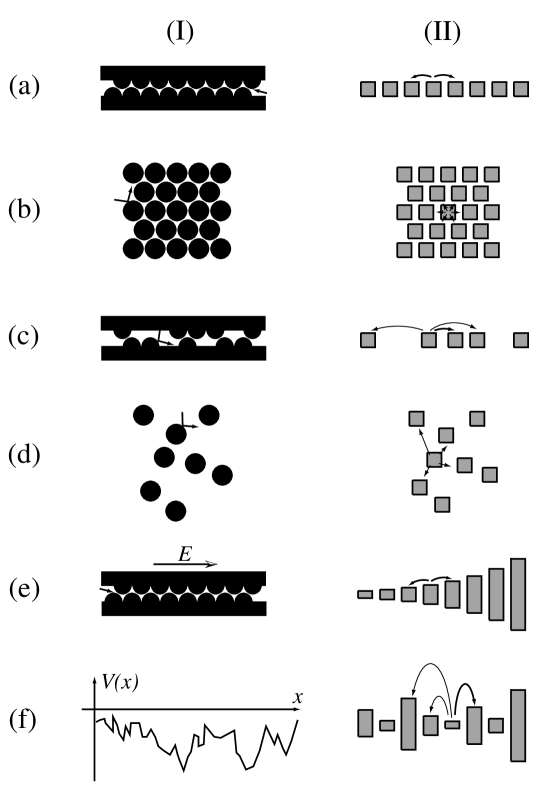
FIG. 3.: Schematic representation of different Lorentz gases (I) and their corresponding multibaker model (II) for configurations of scatterers which are: (a) one-dimensional and periodic; (b) two-dimensional and periodic; (c) one-dimensional and disordered; (d) two-dimensional and disordered; (e) with a constant electric field $E$; (f) with a disordered potential $V(x)$. In each example of column (II), the multibaker map acts on the grey squares or rectangles by a baker-type transformation combined with translations (depicted by arrows) of the cut pieces to the neighboring squares or rectangles. The multibaker (IIa) is defined by Eqs. (112) and (113).

A dyadic version of the multibaker map is defined by the following mapping which acts on a chain of unit squares [16]

$$\phi(x,y)\ =\ \cases{\Bigl{(}2x,{y\over 2}\Bigr{)}\ ,\qquad\qquad\ \ 0\leq x\leq{1\over 2}\;,\cr\Bigl{(}2x-1,{{y+1}\over 2}\Bigr{)}\ ,\qquad{1\over 2}<x\leq 1\;,\cr}$$ (112)

with the jump vector

$$L(x,y)\ =\ \cases{-\alpha\;,\qquad 0\leq x\leq{1\over 2}\;,\cr+\alpha\;,\qquad{1\over 2}<x\leq 1\;,\cr}$$ (113)

where $\alpha$ is the spatial distance separating two neighboring squares. The dynamics of the multibaker is time-reversal symmetric under the involution $I(x,y)=(1-y,1-x)$ so that $\phi^{-1}=I\circ\phi\circ I$. The dyadic multibaker (112) is hyperbolic with the positive Lyapunov exponent $\ln 2$ and chaotic with the KS entropy $h_{\rm KS}=\ln 2$. It is also area-preserving as is the Birkhoff map, and the coordinates $(0<x<1,0<y<1)$ play a similar role as the Birkhoff coordinates $(\theta,\varpi)$. They also form a pair of canonically conjugate variables. On the other hand, the coordinate $x$ corresponds to the unstable direction of the mapping and the coordinate $y$ to its stable direction. This is not the case for the Birkhoff coordinates $(\theta,\varpi)$ which mix the stable and unstable directions of the Birkhoff mapping. Therefore, if the linearization of the Birkhoff map of the hard-disk Lorentz gas were possible, a change of variables would be required to relate the Birkhoff coordinates $(\theta,\varpi)$ to the multibaker coordinates $(x,y)$. The Birkhoff map of the hard-disk Lorentz gas has singularity lines connected to grazing collisions which are absent in the multibaker map. In this regard, the multibaker map constitutes an important simplification of the Birkhoff map of the hard-disk dynamics but the analogy is complete as far as all the other properties are concerned, such as the dimensionality of the phase space, the diffusivity of the particles moving under the multibaker dynamics, the area-preserving property, as well as the positivity of the Lyapunov exponent. It is possible to take into account the energy of the particle in the multibaker model by simply keeping this variable as in the Lorentz gas as explained in Refs. [17, 18, 27]. In analogy with the Lorentz gas, energy is conserved. Moreover, we may suppose that the path length between two successive intersections in the plane $(x,y)$ of the multibaker map is independent of the coordinates $(x,y)$ and takes the constant value $\Lambda(x,y)=\Lambda_{c}$.

In the multibaker map, the phase space is based on a chain of squares. Each square of it is stretched, cut in two pieces, and mapped on the neighboring squares. The multibaker is mixing, as is the hard-disk Lorentz gas so that a local equilibrium is established in each square of the chain because the dynamics randomizes the coordinates $(x,y)$. Moreover, this mapping induces jumps of the particle along the chain of squares. The jumps generate a symmetric random walk with diffusion coefficient ${\cal D}=v(\epsilon)\alpha/2$, where $v(\epsilon)$ is the speed of the particles which may be supposed to be the same as in the hard-disk Lorentz gas.

B The thermodynamics of the multibaker map

Except that the dynamics is simplified, the physical interpretation of the multibaker map of diffusion is similar to the one of the corresponding Lorentz gas. Thus the thermodynamic considerations of the previous section apply mutatis mutandis. Let us consider a gas of $N_{1}$ particles in a multibaker chain containing $N_{2}$ squares. We can impose periodic boundary conditions at the ends of the chain for instance. The phase space of the $N_{1}$ particles is

$${\cal M}=\{(\ell_{1},x_{1},y_{1},\lambda_{1},\epsilon_{1},...,\ell_{N_{1}},x_{N_{1}},y_{N_{1}},\lambda_{N_{1}},\epsilon_{N_{1}})|\ell_{1}+x_{1}<...<\ell_{N_{1}}+x_{N_{1}}\}\;,$$ (114)

with $\ell_{j}\in\{1,2,3,...,N_{2}\}$, $0<x_{j}<1,0<y_{j}<1,0<\lambda_{j}<\Lambda_{c},0<\epsilon_{j}$, with, again, the ordering required by the indistinguishability of the particles. In this phase space, the equilibrium microcanonical probability distribution has the following density function

$$F(x_{1},y_{1},\lambda_{1},\epsilon_{1},...,x_{N_{1}},y_{N_{1}},\lambda_{N_{1}},\epsilon_{N_{1}})=\cases{\frac{\displaystyle N_{1}!}{\displaystyle{\cal V}^{N_{1}}\Delta\epsilon^{N_{1}}}\qquad{\rm for}\quad\epsilon<\epsilon_{j}<\epsilon+\Delta\epsilon\;,\cr\cr 0\qquad{\rm otherwise}\;,\cr}$$ (115)

where $\cal V$ is the volume of the domain where the light particles move. This volume can be supposed to depend on the physical volume $V$ and on the number $N_{2}$ of hard disks as in the corresponding Lorentz gas. The equilibrium Gibbs entropy (62) calculated for this distribution function is given by

$$S=k_{\rm B}N_{1}\;\ln\frac{{\cal V}\;{\rm e}}{N_{1}\Delta x\Delta y\Delta\lambda}\;,$$ (116)

where $\Delta x\Delta y\Delta\lambda\Delta\epsilon$ is the volume of the cells partitioning the phase space. The Gibbs relation (65) is satisfied with a vanishing inverse temperature, the chemical potential of the light particles given by

$$\frac{\mu_{1}}{\cal T}=k_{\rm B}\ln\frac{N_{1}\Delta x\Delta y\Delta\lambda}{{\cal V}}\;,$$ (117)

and another one for the scatterers

$$\frac{\mu_{2}}{\cal T}=\frac{N_{1}k_{\rm B}}{\cal V}\left(-\frac{\partial{\cal V}}{\partial N_{2}}\right)\;.$$ (118)

Hence, the considerations of the previous section follow, showing that the multibaker map is also consistent with the irreversible thermodynamics of diffusion processes, contrary to the claims by Cohen and Rondoni [29].

In Refs. [17, 18, 20, 23, 24, 25, 26, 27, 53, 54], the entropy production associated with the transport processes sustained by multibaker models was derived and the expressions expected from irreversible thermodynamics have been obtained. More recently, the ab initio derivation of entropy production of diffusion has been extended to the continuous-time dynamics of the Lorentz gas as well as to many-body systems composed of a tracer particle moving in a fluid of other particles [55]. These works show that the thermodynamically expected entropy production can be successfully derived from dynamics in the Lorentz gases and multibaker maps.

V Conclusions

This paper provides counter-arguments refuting the doubts and criticisms expressed by Cohen and Rondoni concerning the thermodynamic considerations of Lorentz gases and multibaker maps. We have shown that their claims cannot be taken uncritically, and do not stand up under a rather direct consideration of the irreversible thermodynamics of isothermal mixing of distinct chemical species. We hope that this exchange of ideas will be helpful for clarifying the thermodynamics of the model systems we study. We feel that, at best, the arguments of Cohen and Rondoni should be considered as restatements of the facts that a study of simple systems may not reveal all of the features and difficulties that one encounters in a study of complicated ones. Yet, whatever the specificities of simple systems may be, we have seen that they remain within the realm of irreversible thermodynamics. The present work thus shows that irreversible thermodynamics indeed has a universal applicability in the class of spatially-extended many-particle systems.

We should point out that the goal of the line of research presented in the papers criticized by Cohen and Rondoni is not the treatment of entropy production in Lorentz gases or multi-baker maps. Rather, these papers represent steps on the way to a treatment of entropy production in classical fluids. As is often the case in statistical physics, the study of simple models allows workers to develop insights into the ideas and techniques needed to treat more realistic systems. From this point of view the criticisms of Cohen and Rondoni, while mistaken, as we argue here, would also be irrelevant if our line of research shows that similar methods can be useful in the study of fluid systems where all of the particles can interact with each other. In fact, we have shown in a previous paper [55], that the methods under discussion apply equally well to a periodic, fluid system with a tracer particle. In this case, we considered a fully interacting, periodic $N+1$ particle system, in a microcanonical ensemble. For this system the presence of interacting, moving particles does not change the arguments in any important way.

Cohen and Rondoni have also raised more technical objections to our use of Sinai-Ruelle-Bowen measures to calculate the rate of entropy production as described in Refs. [14, 20, 53, 54, 55] which also require a response. This will be supplied in a future publication.

Acknowledgments. The authors thank Doron Cohen, E. G. D. Cohen, T. Gilbert, H. Larralde, L. Rondoni, H. van Beijeren, J. Vollmer, and D. Wojcik for interesting and helpful discussions. PG thanks the National Fund for Scientific Research (FNRS Belgium) for financial support. JRD thanks the National Science Foundation (USA) for support under grant PHY-98-20824.

REFERENCES

- [1] H. A. Lorentz, Proc. Roy. Acad. Amst. 7 (1905) 438, 585, 684.
- [2] H. van Beijeren, Rev. Mod. Phys. 54 (1982) 195.
- [3] C. P. Dettmann, The Lorentz gas as a paradigm for nonequilibrium stationary states, in: D. Szasz, Editor, Hard Ball Systems and Lorentz Gas, Encycl. Math. Sci., Springer, Berlin, 2000.
- [4] S. Chapman and T. G. Cowling, The Mathematical Theory of Non-uniform Gases, 3rd. ed., Cambridge University Press, Cambridge UK, 1970, Chap. 10.
- [5] E. H. Hauge, in: Transport Phenomena, G. Kirczenow and J. Marro, Eds., Springer-Verlag, Berlin, 1974.
- [6] L. A. Bunimovich and Ya. G. Sinai, Commun. Math. Phys. 78 (1980) 247, 479.
- [7] A. Knauf, Commun. Math. Phys. 110 (1987) 89; Ann. Phys. (N. Y.) 191 (1989) 205.
- [8] N. I. Chernov, G. L. Eyink, J. L. Lebowitz, and Ya. G. Sinai, Phys. Rev. Lett. 70 (1993) 2209.
- [9] N. I. Chernov, G. L. Eyink, J. L. Lebowitz, and Ya. G. Sinai, Comm. Math. Phys. 154 (1993) 569.
- [10] P. Gaspard, J. Stat. Phys. 68 (1992) 673.
- [11] V. I. Arnold and A. Avez, Ergodic Problems of Classical Mechanics, Benjamin, New York, 1968.
- [12] E. Hopf, Ergodentheorie, Springer-Verlag, Berlin, 1937.
- [13] W. Seidel, Proc. Natl. Acad. Sci. USA 19 (1933) 453.
- [14] P. Gaspard, Chaos, Scattering and Statistical Mechanics, Cambridge University Press, Cambridge UK, 1998.
- [15] T. Tél, J. Vollmer, and W. Breymann, Europhys. Lett. 35 (1996) 659.
- [16] S. Tasaki and P. Gaspard, J. Stat. Phys. 81 (1995) 935.
- [17] S. Tasaki and P. Gaspard, Theoretical Chemistry Accounts 102 (1999) 385.
- [18] S. Tasaki and P. Gaspard, J. Stat. Phys. 101 (2000) 125.
- [19] G. Radons, Festkörperprobleme/Advances in Solid State Physics 38 (1999) 339.
- [20] T. Gilbert and J. R. Dorfman, J. Stat. Phys. 96 (1999) 225.
- [21] T. Gilbert, C. D. Ferguson, and J. R. Dorfman, Phys. Rev. E 59 (1999) 364.
- [22] T. Gilbert and J. R. Dorfman, Physica A 282 (2000) 427.
- [23] T. Tél and J. Vollmer, Entropy Balance, Multibaker Maps, and the Dynamics of the Lorentz gas, in: D. Szász, Editor, Hard Ball Systems and the Lorentz Gas, Springer-Verlag, Berlin, 2000, pp. 367-418.
- [24] J. Vollmer, T. Tél, and L. Mátyás, J. Stat. Phys. 101 (2000) 79.
- [25] T. Tél, J. Vollmer, and L. Mátyás, Europhys. Lett. 53 (2001) 458.
- [26] L. Mátyás, T. Tél, and J. Vollmer, Phys. Rev. E 64 (2001) 056106.
- [27] J. Vollmer, Phys. Rep. (to appear).
- [28] L. Rondoni and E. G. D. Cohen, Nonlinearity 13 (2002) 1905.
- [29] E. G. D. Cohen and L. Rondoni, Physica A 306 (2002) 117.
- [30] E. G. D. Cohen and L. Rondoni, Physica D 168-169 (2002) 341.
- [31] L. Mátyás, T. Tél, and J. Vollmer, “Reply to the paper, Particles, Maps, and Irreversible Thermodynamics, by E. G. D. Cohen and L. Rondoni”, (in preparation).
- [32] I. Prigogine, Physica 15 (1949) 272.
- [33] G. Nicolis, J. Wallenborn, and M. G. Velarde, Physica 43 (1969) 263.
- [34] R. Haase, Thermodynamics of irreversible processes, Dover, New York, 1969.
- [35] R. S. Berry, S. A. Rice, and J. Ross, Physical Chemistry, J. Wiley & Sons, New York, 1980.
- [36] S. de Groot and P. Mazur, Non-equilibrium Thermodynamics, North-Holland, Amsterdam, 1962; reprinted by Dover Publ. Co., New York, 1984.
- [37] D. Kondepudi and I. Prigogine, Modern Thermodynamics, J. Wiley, Chichester, 1998.
- [38] G. Nicolis, Rep. Prog. Phys. 42 (1979) 225.
- [39] D. J. Evans and G. Morriss, Statistical Mechanics of Nonequilibrium Liquids, Academic Press, London, 1990.
- [40] W. G. Hoover, Time Reversibility, Computer Simulation, and Chaos, World Scientific, Singapore, 1999.
- [41] J. L. Lebowitz and P. G. Bergmann, Ann. Phys. 1 (1957) 1.
- [42] J. L. Lebowitz, Phys. Rev. 114 (1959) 1192.
- [43] N. I. Chernov and J. L. Lebowitz, Phys. Rev. Lett. 75 (1995) 2831.
- [44] N. I. Chernov and J. L. Lebowitz, J. Stat. Phys. 86 (1997) 953.
- [45] J.-P. Eckmann, C.-A. Pillet, and L. Rey-Bellet, J. Stat. Phys. 95 (1999) 305.
- [46] R. Klages, K. Rateitschak, and G. Nicolis, Phys. Rev. Lett. 84 (2000) 4268.
- [47] C. Boldrighini, L. A. Bunimovich, and Ya. G. Sinai, J. Stat. Phys. 32 (1983) 477.
- [48] J. L. Lebowitz and H. Spohn, J. Stat. Phys. 19 (1978) 633.
- [49] D. Belitz and T. R. Kirkpatrick, Rev. Mod. Phys. 66 (1994) 261.
- [50] N. I. Chernov and C. P. Dettmann, Physica A 279 (2000) 37.
- [51] P. Gaspard, Phys. Rev. 53 (1996) 4379.
- [52] J. W. Gibbs, Elementary Principles in Statistical Mechanics, Yale University Press, New Haven CT, 1902; reprinted by Dover Publ. Co., New York, 1960.
- [53] P. Gaspard, J. Stat. Phys. 88 (1997) 1215.
- [54] T. Gilbert, J. R. Dorfman, and P. Gaspard, Phys. Rev. Lett. 85 (2000) 1606.
- [55] J. R. Dorfman, P. Gaspard, and T. Gilbert, Phys. Rev. E 66 (2002) 026110.
- [56] R. K. Pathria, Statistical Mechanics, Pergamon, Oxford, 1972.