Applicability of the Fisher Equation to Bacterial Population Dynamics

Abstract

The applicability of the Fisher equation, which combines diffusion with logistic nonlinearity, to population dynamics of bacterial colonies is studied with the help of explicit analytic solutions for the spatial distribution of a stationary bacterial population under a static mask. The mask protects the bacteria from ultraviolet light. The solution, which is in terms of Jacobian elliptic functions, is used to provide a practical prescription to extract Fisher equation parameters from observations and to decide on the validity of the Fisher equation.

I  Introduction

Evolution of bacterial colonies is a subject of obvious medical importance and has been studied recently jaco ; waki ; lin ; nels ; thesis experimentally as well as theoretically. Some theoretical descriptions have avoided phenomena such as mutation and have focused on growth, competition for resources, and diffusion. In terms of the respective parameters $a$ (growth rate), $b$ (competition parameter), and $D$ (diffusion coefficient), the basic equation governing the spatio-temporal dynamics of the bacterial population $u\left(x,t\right)$ at a position $x$ and time $t$ has been taken to be the Fisher equation fish

$$\frac{\partial u\left(x,t\right)}{\partial t}=D\frac{\partial^{2}u\left(x,t\right)}{\partial x^{2}}+au\left(x,t\right)-bu^{2}\left(x,t\right).$$ (1)

For simplicity, we consider throughout this paper only the 1-dimensional situation which is indeed appropriate to the observations reported. Experiments have been carried out with moving masks lin and observations have been reported about extinction transitions suggested earlier in theoretical calculations nels and in numerical simulations thesis . Those theoretical calculations have focused on systems in which the growth rate $a$ varies from location to location in a disordered manner, and have employed techniques based on linearization of the Fisher equation. The first feature has allowed the analysis to use concepts from Anderson localization anderson , a phenomenon well-known in solid state physics of quantum mechanical systems. The second feature has relegated the nonlinearity character of Fisher’s equation to a secondary role. Because we suspect nonlinear features represented by $-bu^{2}$ in (1) to be of central importance to bacterial evolution, we have developed a theoretical approach which generally retains the full nonlinearity of that competition term. In the present paper, which is the first of a series built on this approach of maintaining the nonlinearity in the equation, we focus our attention on the effect of a mask on the spatial distribution of the stationary population of the bacteria.

Consider, as in the moving mask experiments lin , an effectively linear petri dish in which a mask shades bacteria from harmful ultraviolet light which kills them in regions outside the mask but allows them to grow in regions under the mask. Unlike in the moving mask experiments, however, consider that the mask does not move but is left stationary. Interest is in the $x$ -dependence of the stationary population of the bacteria. As in previous considerations lin , we will assume that the growth rate has a positive constant value $a$ inside the mask, and a negative value outside the mask.

If we take the value of $a$ outside the mask to be negative infinite to reflect extremely harsh conditions (due to ultraviolet light) when the bacteria are not shaded from the light, we can take the population at the mask edges and outside to be identically zero. We will put $\partial u\left(x,t\right)/\partial t=0$ in (1 ) to reflect stationarity, introduce a scaled position variable $\xi=x/\sqrt{D}$ for simplicity, and begin our analysis with the ordinary differential equation for the stationary population $u\left(\xi\right)$:

$$\frac{d^{2}u\left(\xi\right)}{d\xi^{2}}+au\left(\xi\right)-bu^{2}\left(\xi\right)=0.$$ (2)

Our interest is in the regions in the interior of the mask of width $2w$, i.e., for $-w\leq x\leq w,$ the boundary conditions being $u\left(\pm w/\sqrt{D}\right)=0.$

The purpose of our investigation is to give a practical prescription to decide on the applicability of the Fisher equation to bacterial evolution, and to extract the parameters $D,\,a,\,b$ from observations if the equation is found to be applicable.

II Elliptic Solutions in the Interior and Extraction of Fisher Parameters

The solutions of (2) can be written in terms of Jacobian elliptic functions as follows. It is known ellip that the square of any of cn$(\xi,k)$, sn$(\xi,k)$ or dn$(\xi,k)$, satisfies an equation resembling (2). Here, we use the notation that $k$ is the elliptic parameter defi rather than the elliptic modulus which is the square of $k$. Thus, $y=$ $\mbox{sn}^{2}(\xi,k)$ is known to satisfy

$$\frac{d^{2}y}{d\xi^{2}}+4\left(1+k^{2}\right)y-6k^{2}y^{2}=2.$$ (3)

Comparison of (3) with (2) shows that the signs of the linear and quadratic coefficients are the same in the two equations but (3) has an extra constant term on the right hand side. This difference, as well as the fact that the bacterial system has more independent parameters than the single $k$ that appears in (3), suggests that we augment $\mbox{sn}^{2}(x,k)$ by phase and amplitude parameters, i.e., take as the solution of (2) within the mask

$$u_{i}\left(\xi\right)=\alpha\,\mbox{sn}^{2}\left(\beta\xi+\delta,k\right)+\gamma,$$ (4)

and obtain the quantities $\alpha,\beta,\delta,\gamma$ by differentiating (4) or by other means. The suffix $i$ represents the interior of the mask. Symmetry considerations, specifically the requirement that the maximum of $u_{i}\left(\xi\right)$ be at $\xi=0,$ lead to an evaluation of $\delta$ as half the period of $\mbox{sn}^{2}$. A shift identity allows the rewriting of (4) as

$$u_{i}\left(\xi\right)=\alpha\,\mbox{cd}^{2}\left(\beta\xi,k\right)+\gamma,$$ (5)

the cd function ellip being simply the ratio $\mbox{cn}/\mbox{sn}.$

On differentiating (5) twice w.r.t. $x$, using the relationships among the elliptic functions, and substituting in (2), we find:

$$4\beta^{2}(k^{2}+1)-a+2b\gamma = 0,$$

$$6k^{2}\beta^{2}-b\alpha = 0,$$

$$2\alpha\beta^{2}(1-k^{2})+\gamma(a-\gamma b) = 0.$$

Solution of this algebraic system leads to the result that $\alpha$ and $\gamma$ are proportional to each other through a factor which is a function only of the elliptic parameter,

$$\gamma=\alpha\left[\frac{-\left(k^{2}+1\right)+\sqrt{1-k^{2}+k^{4}}}{3k^{2}}\right].$$

We also find explicit connections between the quantities $\alpha,\beta\$ and two of the Fisher parameters of the bacterial system $a,b,$

$$\begin{array}[]{lll}\alpha&=&\left(\frac{3a}{2b}\right)k^{2}\left(1-k^{2}+k^{4}\right)^{-1/2}\\ \beta^{2}&=&\left(\frac{a}{4}\right)\left(1-k^{2}+k^{4}\right)^{-1/2}.\end{array}$$ (6)

This allows us to write the stationary solution as

$$u_{i}\left(\xi\right)=\left(a/b\right)\left[\,f_{\alpha}\left(k\right)\mbox{cd}^{2}\left(\sqrt{a}f_{\beta}\left(k\right)\xi,k\right)+f_{\gamma}\left(k\right)\right]$$ (7)

explicitly in terms of the Fisher parameters $a,b$ and three functions of $k$ alone:

$$f_{\alpha}\left(k\right) = \left(3/2\right)k^{2}\left(k^{\prime 2}+k^{4}\right)^{-1/2}$$

$$f_{\beta}\left(k\right) = \left(1/2\right)\left(k^{\prime 2}+k^{4}\right)^{-1/4}$$

$$f_{\gamma}\left(k\right) = \left(1/2\right)\left[1-\left(k^{2}+1\right)\left(k^{\prime 2}+k^{4}\right)^{-1/2}\right].$$ (8)

Here $k^{\prime 2}=1-k^{2}.$

Equation (7) provides us with the means to meet the primary goal of this investigation. The practical prescription we seek for investigating the applicability of the Fisher equation begins with fitting (7) to the observed stationary profile. A least-squares procedure yields $a,b,k$. For sensitivity purposes we use the nome $q=\exp\left(-\pi K^{\prime}/K\right)$ for fitting nome rather than $k.$ The relation

$$u_{m} = \frac{a}{b}\left[\,f_{\alpha}\left(k\right)+f_{\gamma}\left(k\right)\right]$$

$$= \frac{a}{2b}\left(k^{2}-\,k^{\prime 2}+(k^{{}^{\prime}2}+k^{4})^{1/2}\right)(k^{\prime 2}+k^{4})^{-1/2}$$

between the maximum value of the bacterial population $u_{m}$ and the extracted parameters provides a check on the procedure. The determination of the diffusion constant $D$ follows the determination of $k.$ For this we can use the boundary condition mentioned above, that $u(\xi)$ vanishes at the edges of the mask: $\xi=\pm w/\sqrt{D}.$ Equation (7) leads then to an implicit expression which yields the diffusion constant $D:$

$$\mbox{cn}^{2}\left(\left(a/4\right)\left(1-k^{2}+k^{4}\right)^{-1/2}w/\sqrt{D},k\right)=\,$$ (10)

$$\frac{\left[(\left(k^{2}+1\right)-\left(1-k^{2}+k^{4}\right)^{1/2})(1-k^{2})\right]}{k^{2}(2-k^{2}+\left(1-k^{2}+k^{4}\right)^{1/2})}.$$

Our prescription for the extraction of Fisher parameters $D$, $a$, $b$ is, thus, complete provided we can assume the conditions outside of the mask to be harsh enough to put $u$ at the edges to vanish. This assumption can be tested from the observations. The question of the very applicability of the Fisher equation to the bacterial system can be addressed by the quality of the fits of solution to the data. Fits of poor quality would necessitate a rethinking of the quadratic nonlinearities assumed in the equation, indeed of the entire form of the equation.

We illustrate our practical prescription in Fig. 1. We have considered two hypothetical cases of the observed stationary profile of he bacterial population. One pertains to a situation in which the Fisher equation is applicable: (1a); the other in which it is not: (1b). The ‘data’ correspond, respectively, to stationary solutions of (1) and of the so-called Nagumo equation kot

$$\frac{\partial u}{\partial t}=D\frac{\partial^{2}u}{\partial x^{2}}+\left(u-C\right)\left(Au-Bu^{2}\right),$$ (11)

noise having been added in each case to simulate experiments.

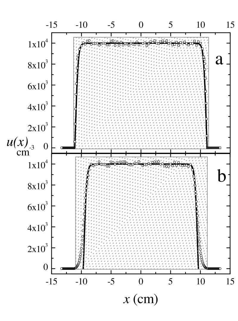
Figure 1: Procedure to determine applicability of Fisher equation and/or to extract parameters from observations. Shown is a least-squares fitting of the analytic solution, Eq(7), of the Fisher equation, to numerically generated ‘data’ by adding noise to theoretical predictions in two cases. In a) the Fisher equation can be considered applicable while in b) it cannot.

The numerically generated data are plotted with circles while the full line curve shows the best fit. We see that in Fig. 1a, the Fisher solution matches well the data. By contrast, the fitting procedure fails in 1b. The intrinsic non-linearities in the data of 1b are different from those characteristic of the Fisher equation (compare Eqs. (1) and (11)). Some of the data features in 1b, as for example the change in concavity and the zero derivative at the borders of the mask can not be reproduced by the analytic solution Eq (7). Thus, we have shown here how one would determine clearly the applicability of the Fisher equation to a given set of observations.

How would one proceed if, in the light of experiment, the Fisher equation turns out to be inapplicable in this way? We suggest an additional prescription to obtain the form of the nonlinearity from the stationary mask observations. The observed stationary bacterial profile is $u_{i}\left(x\right).$ A numerical differentiation procedure can be made to produce $d^{2}u_{i}\left(x\right)/dx^{2}.$ A plot of $d^{2}u_{i}\left(x\right)/dx^{2}$ versus $u_{i}\left(x\right),$ the different points corresponding to different values of $x$, would either confirm Fisher behavior or point to nonlinearities, such as that in the Nagumo equation, other than that assumed in the Fisher equation. Fig. 2 illustrates this prescription in the context of the assumed observations in Fig. 1a and Fig. 1b. The ‘data’ were numerically differentiated in each case and the second spatial derivative was plotted versus $u$ as shown simple .

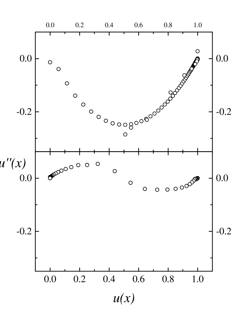
Figure 2: Procedure to extract from experiment the type of non-linearity in bacterial evolution. Numerically obtained second derivative of $u$ is plotted against $u$ in the two cases a and b of Fig. 1.

While the quadratic nonlinearity characteristic of the Fisher equation is compatible with Fig 2a, the curvature of the data in Fig. 2b immediately points out the incompatibility with the Fisher equation and suggests a Nagumo-like alternative.

III Dependence on Mask Size

Obviously, good experimental practice should use for the extraction of the Fisher parameters not a single mask but masks of varying sizes. It is clear that the peak value of the profile, $u_{m},$ will decrease as the mask size is decreased (alternatively as the diffusion coefficient is increased). However, what is the precise dependence of the stationary profile on the size of the mask, as the size is varied? In answering this question, one finds that the peculiarities of the elliptic solutions produce a bifurcation behavior: there is a minimum mask size below which bacteria cannot be supported because they diffuse into the harsh regions where they die. We suggest that this effect, known in the study of phytoplankton blooms kot , be used to validate the Fisher equation in bacterial population as follows.

The dependence of the peak value of the stationary bacterial population on $k$ is in (II) whereas the dependence of the mask width $2w$  on $k$ is obtained by inverting (10)

$$\begin{array}[]{rcl}w&=&\frac{\sqrt{D}}{\left(a/4\right)\left(1-k^{2}+k^{4}\right)^{-1/2}}\\ &&\mbox{cn}^{-1}\left(\left(\frac{\left[(\left(k^{2}+1\right)-\left(1-k^{2}+k^{4}\right)^{1/2})(1-k^{2})\right]}{k^{2}(2-k^{2}+\left(1-k^{2}+k^{4}\right)^{1/2})}\right)^{1/2}|k\right).\end{array}$$ (12)

The conjunction of (II) and (12) yield the dependence of the profile peak on the mask size. For a given set of Fisher parameters, a decrease in the mask width $2w$ from large values causes a decrease in $k$. This decrease is monotonic. The value $k=0$ is reached at a finite value of the width. In this limit, the elliptic function cd$(\beta\xi,k)$ becomes its trigonometric counterpart cos$(\beta\xi)$, and (10) reduces to

$$\cos^{2}\left(\frac{w}{2}\sqrt{a/D}\right)=0.5.$$ (13)

Thus, there is a critical size $2w_{c}$ of the mask:

$$2w_{c}=\pi\sqrt{\frac{D}{a}}.$$ (14)

No stationary bacterial population can be supported below such a size. An excellent experimental check on the applicability of the Fisher equation could be the determination of this bifurcation behavior. On the basis of quoted lin ; thesis values $D\approx 10^{-5}$ cm²/s, $a\approx 10^{-4}$/s, we obtain the critical mask size to be of the order of half a cm, a limit that should be observable.

Figure 3: Reduction of the critical size of the mask as a result of the finiteness of $a$ outside the mask. Shown as (a) is the dependence of the maximum of the profile, $u_{m}$, on the width of the mask. For comparison we give (b), the $u_{m}$ dependence on $2w$ in the Dirichlet case. For case (a), the inset shows the actual profiles for several values of the width.

If we relax the condition that the environment outside the mask is harsh enough to ensure zero population of the bacteria, Dirichlet boundary conditions used in the previous analysis are not appropriate. In the steady state, the bacterial concentration just outside the borders of the mask would then be different from zero as a result of finite diffusion. While the elliptic function solution in Eq. (7) (but without the Dirichlet boundary condition) is appropriate inside the mask, it turns out to be exceedingly difficult to find a solution outside the mask. If one starts out with the same (elliptic) form of the solution outside but with a negative but finite value of $a,$ one gets the requirement that $u\left(\xi\right)$ be negative. This is not allowable since $u\left(\xi\right)$ is a bacterial density which must remain positive. Other known solutions

$$u(\xi)=-\frac{\left(3/2\right)\left(a/b\right)}{\cosh^{2}\left(\frac{\sqrt{a}\xi}{2}\right)}$$ (15)

are also rejected on account of their patent negativity. It is possible, however, to obtain reasonable solutions lud if it is assumed that the bacterial densities outside the mask are so small that the quadratic term proportional to $b$ may be neglected in the Fisher equation for the analysis in the exterior of the mask. Such an analysis leads to a smaller critical size relative to that in (14). Fig. 3 shows the dependence of $u_{m}$ on mask size for both the cases of (a) infinite and (b) finite (b) (negative) $a$ outside the mask. The inset shows the $x$ dependence of the solution for the latter case.

IV Remarks

Our interest in the present paper being in the determination of the applicability of the Fisher equation to experiments currently being conducted on the bacterial evolution in Petri dishes, we have displayed the explicit solution (7) to the Fisher equation (2) in the infinite-time limit when a stationary mask of given width shades the bacteria under it from harsh conditions outside it. Such stationary mask experiments we propose are easier and more direct for the purposes of determination of the validity of the Fisher equation, and for the extraction of the parameters of the equation. It is our suggestion that parameters extracted in this manner may be used subsequently for the analysis of moving mask experiments lin , with greater confidence in the reliability of the parameter values.

We have indicated explicitly how the extraction of the Fisher parameters may be carried out. The numerical fitting procedure in Fig. 1a shows the parameters relevant to the hypothetical observations to be $D=10^{-5}$cm²/s , $a=10^{-4}$/s, $b=10^{-8}$ cm³/s and $w=11$ cm, while the nome $q=0.8071$ foot . The procedure does produce parameter values when applied to Fig. 1b but the quality of the fits is poor. Such a situation would signal the inapplicability of the Fisher equation. The ‘data’ in Fig. 1b have been generated from the Nagumo equation whose intrinsic nonlinearities are incompatible with those of the Fisher equation as is visually clear from the best fits. We have shown in Fig. 2 how general manipulations of the observed data may be used to suggest the particular form of nonlinearity to be used in the model. We have also concluded that the critical size effect which arises directly from the solution (7) is probably within observable limits for bacterial evolution, the size we predict in light of quoted parameters being of the order of 0.5 cm. This conclusion would necessitate modification if the actual values of $D$ and $a$ are different from those currently believed.

In forthcoming publications we will report our analyses of the spatio-temporal behavior of the bacterial population of relevance to time-dependent experiments. Our basis is the Fisher equation KK and several interesting alternatives such as a formalism in which diffusion is negligible but coherent motion is present GK , and a formalism in which long-range competition interactions produce an influence function and consequently striking patterns FKK in bacterial populations.

V Acknowledgements

This work is supported in part by the Los Alamos National Laboratory via a grant made to the University of New Mexico (Consortium of The Americas for Interdisciplinary Science) and by National Science Fundation’s Division of Materials Research via grant No DMR0097204.

References

- (1) E. Ben-Jacob, I. Cohenand H. Levine. Adv. Phys. 49 ,395-554 (2000)
- (2) J. Wakita, K. Komatsu, A. Nakahara, T Matsuyama, M. Matsushita. Journ. Phys. Soc. Japan 63, 1205 (1994).
- (3) A. L. Lin, B. Mann, G. Torres, B. Lincoln, J. Kas and H. L. Swinney, "Localization and extinction of bacterial populations under inhomogeneous growth conditions", preprint.
- (4) D.R. Nelson and N.M. Shnerb, Phys. Rev. E 58,1383 (1998); K.A. Dahmen, D.R. Nelson and N.M. Shnerb, J. Math Biology, 41,1 (2000).
- (5) B. Mann, Spatial phase transitions in bacterial growth, Ph.D. Thesis (2001), unpublished.
- (6) R.A.Fisher, Ann. Eugen. London 7, 355-369 (1937).
- (7) P.W. Anderson, Phys. Rev. 109, 1492 (1958).
- (8) F. Bowman. Introduction to elliptic functions. Dover, New York. (1961), see also G. Abramson, A. Bishop and V. Kenkre, Physica A, 305, 427-436 (2002).
- (9) Thus, means that .
- (10) The quantities and are functions of defined as and
- (11) M. Kot. Elements of Mathematical Ecology. Cambridge U.P. (2001).
- (12) Simple polynomials in were used for the fitting of the data to assist in the numerical differentiation.
- (13) D. Ludwig, D.G. Aronson and H.F. Weinberger. J. Math. Biology 8, 217-258 (1979).
- (14) M. N. Kuperman and V. M. Kenkre, “Moving Mask Analysis of Bacteria in a Petri Dish”, preprint.
- (15) L. Giuggioli and V. M. Kenkre, “Analytic Solutions of Nonlinear Convective Diffusion Equations for Population Dynamics of Bacteria and Related Systems", preprint.
- (16) M. Fuentes, M. N. Kuperman and V. M. Kenkre, “Influence Functions in Fisher-like Equations and the Formation of Spatial Patterns”, preprint.
- (17) The fitting in Fig. 1 corresponds to cm. While this value appears larger than those used in current experiments, the values of and quoted in the literature have considerable uncertainty at the present moment.