S

maller alignment index (SALI): Determining the ordered or chaotic nature of orbits in conservative dynamical systems

s) Ch. Skokos^a,b, Ch. Antonopoulos^a, T. C. Bountis^a & M. N. Vrahatis^c

^aDepartment of Mathematics, Division of Applied Analysis and Center for Research and Applications of Nonlinear Systems (CRANS),
University of Patras, GR-26500 Patras, Greece
^bResearch Center for Astronomy, Academy of Athens, 14 Anagnostopoulou str., GR-10673 Athens, Greece
^cDepartment of Mathematics and University of Patras Artificial Intelligence Research Center (UPAIRC),
University of Patras, GR-26110 Patras, Greece

Abstract

We apply the smaller alignment index (SALI) method for distinguishing between ordered and chaotic motion in some simple conservative dynamical systems. In particular we compute the SALI for ordered and chaotic orbits in a 2D and a 4D symplectic map, as well as a two–degree of freedom Hamiltonian system due to Hénon & Heiles. In all cases, the SALI determines correctly the nature of the tested orbit, faster than the method of the computation of the maximal Lyapunov characteristic number. The computation of the SALI for a sample of initial conditions allows us to clearly distinguish between regions in phase space where ordered or chaotic motion occurs.

1 Introduction

One of the most important approaches for understanding the behavior of a dynamical system is based on the knowledge of the chaotic vs. ordered nature of its orbits. For Hamiltonian systems with two degrees of freedom (or equivalently for 2D symplectic maps), the inspection of the consequents of an orbit on a Poincaré surface of section (PSS), can give us reliable information for the dynamics of individual orbits. On the other hand, the distinction between ordered and chaotic motion becomes particularly difficult in systems with many degrees of freedom, where phase space visualization is no longer easily accessible. A quantitative method for distinguishing between order and chaos that has been extensively used (also for multidimensional systems), is the computation of the maximal Lyapunov characteristic number (LCN) [1, 3]. The LCN is the limit of the finite time Lyapunov characteristic number:

$$L_{t}=\frac{1}{t}\,\ln\frac{|\xi_{t}|}{|\xi_{0}|}$$ (1)

(where $\xi_{0}$ and $\xi_{t}$ are the distances between two points of two nearby orbits at times $t=0$ and $t$), when $t$ tends to infinity. In other words, LCN measures the average exponential deviation of two nearby orbits, so if LCN=0 the tested orbit is ordered and if LCN $>0$ it is chaotic. In maps, $t$ is a discrete variable i.e. the number $N$ of iterations of the map, so the finite time Lyapunov characteristic number can be denoted as $L_{N}$. An advantage of this method is that it can be applied to systems of any number of degrees of freedom. The main disadvantage of LCN is that the time needed for $L_{t}$ to converge to its limit can be extremely high and in some cases even unrealistic for the systems under study. A fast, efficient and easy to compute criterion to check if orbits of multidimensional maps are chaotic or not has been introduced in [5]: It concerns the computation of the smaller alignment index (SALI). Recently this method has been successfully applied to a two–degree of freedom Hamiltonian flow [7]. In the present communication we first recall the definition of the SALI and show its effectiveness by applying it to a 2D and a 4D symplectic map, comparing it also to the computation of LCN. We then use the SALI to study the dynamics of the Hénon–Heiles Hamiltonian system; and illustrate its ability to distinguish between regions of the phase space where ordered and chaotic motion occurs clearly and faster than LCN.

2 Definition of the smaller alignment index (SALI)

Let us consider the $2n$–dimensional phase space of a conservative dynamical system, described by a symplectic map T or a Hamiltonian system defined by the $n$ degrees of freedom Hamiltonian function $H$. The time evolution of an orbit with initial condition $P(0)=(x_{1}(0),\;x_{2}(0),\dots,\;x_{2n}(0))$ is defined by the repeated applications of the map T or by the solution of Hamilton’s equations of motion. In order to find the LCN one has to compute the limit of the finite time Lyapunov characteristic number $L_{t}$ (1) for an initially infinitesimal deviation vector $\xi(0)=(dx_{1}(0),\;dx_{2}(0),\dots,\;dx_{2n}(0))$, as the time $t$ or the number of iterations $N$ tend to infinity, for Hamiltonian flows and maps respectively. The time evolution of the deviation vector is given by the equations of the tangent map

$$\xi(N+1)=\left(\frac{\partial\mbox{\bf T}}{\partial P(N)}\right)\xi(N),$$ (2)

for maps, and by the variational equations

$${\bf J}\cdot\dot{\xi}^{\prime}={\bf DH}\cdot\xi^{\prime},$$ (3)

for flows, where (^′) denotes the transpose matrix and matrices ${\bf J}$ and ${\bf DH}$ are defined by

$${\bf J}=\left(\begin{array}[]{ccc}{\bf 0_{n}}&{\bf-I_{n}}\\ {\bf I_{n}}&{\bf 0_{n}}\end{array}\right)\;\;,\;\;DH_{ij}=\frac{\partial^{2}H}{\partial x_{i}\,\partial x_{j}}\;\;\mbox{with}\;\;i,j=1,2,...,2n,$$ (4)

${\bf I_{n}}$ being the $n\times n$ identity matrix and ${\bf 0_{n}}$ the $n\times n$ matrix with all its elements equal to zero. In order to define the SALI for the orbit with initial conditions $P(0)$ we follow the time evolution of two initial deviation vectors $\xi_{1}(0)$ and $\xi_{2}(0)$. At every time step we normalize each vector to $1$ and define the parallel alignment index

$$d_{-}(t)\equiv\|\xi_{1}(t)-\xi_{2}(t)\|$$ (5)

and the antiparallel alignment index

$$d_{+}(t)\equiv\|\xi_{1}(t)+\xi_{2}(t)\|,$$ (6)

following [5] ($\|\cdot\|$ denotes the Euclidean norm of a vector). The smaller alignment index SALI is given by

$$\mbox{SALI}=\min(d_{-}(t),d_{+}(t)).$$ (7)

From the above definitions we see that when the two vectors $\xi_{1}(t)$, $\xi_{2}(t)$ tend to coincide we get

$$d_{-}(t)\rightarrow 0,\;d_{+}(t)\rightarrow 2,\;\mbox{SALI}\rightarrow 0,$$

while, when they tend to become opposite we get

$$d_{-}(t)\rightarrow 2,\;d_{+}(t)\rightarrow 0,\;\mbox{SALI}\rightarrow 0.$$

So, it is evident that SALI is a quantity that clearly informs us if the two deviation vectors tend to have the same direction by coinciding or becoming opposite. The reason why this information is useful for understanding if an orbit is chaotic or not is that, for systems of $2n$–dimensional phase space with $n\geq 2$, the two vectors tend to coincide or become opposite for chaotic orbits [8], i.e. the SALI tends to zero. This is due to the fact that the direction of the two deviation vectors tends to coincide with the direction of the most unstable nearby manifold. On the other hand, if the tested orbit is ordered it lies on a torus and the two deviation vectors eventually become tangent to the torus, but in general converge to different directions. In that case the SALI does not tend to zero, but its values fluctuate around a positive value. Although the SALI method is perfectly suited for multidimensional systems, it can also be applied to 2D maps. For 2D maps, whose phase space is 2–dimensional, the SALI tends to zero both for ordered and chaotic orbits, but with completely different time rates which allows us to clearly distinguish between the two cases. This behavior is due to the fact that for ordered orbits the two vectors, as has already mentioned, become tangent to the torus, which now is simply an invariant curve. So, the only possibilities for the two vectors are to become identical or opposite which means that the SALI tends to zero.

3 Applications of the SALI

3.1 Symplectic maps

Following [5] we compute the SALI in some simple cases of ordered and chaotic orbits in symplectic maps with two and four dimensions. In particular we use the 2D map:

$$\begin{array}[]{lll}x^{\prime}_{1}&=&x_{1}+x_{2}\\ x^{\prime}_{2}&=&x_{2}-\nu\sin(x_{1}+x_{2})\end{array}\pmod{2\pi},$$ (8)

and the 4D map:

$$\begin{array}[]{l}x^{\prime}_{1}=x_{1}+x_{2}\\ x^{\prime}_{2}=x_{2}-\nu\sin(x_{1}+x_{2})-\mu[1-\cos(x_{1}+x_{2}+x_{3}+x_{4})]\\ x^{\prime}_{3}=x_{3}+x_{4}\\ x^{\prime}_{4}=x_{4}-\kappa\sin(x_{3}+x_{4})-\mu[1-\cos(x_{1}+x_{2}+x_{3}+x_{4})]\end{array}\pmod{2\pi},$$ (9)

which is composed of two 2D maps of the form (8), with parameters $\nu$ and $\kappa$, coupled with a term of order $\mu$. All variables are given (mod $2\pi$), so $x_{i}\in[-\pi,\pi),$ for $i=1,2,3,4$. The map (9) is a variant of the 4D map studied by Froeschlé [2]. Some dynamical structures on the phase space of this map were examined in detail in [6] for small values of the coupling parameter $\mu$.

Figure 1: (a) Phase plot of the 2D map (8) for $\nu=0.5$. The initial conditions of the ordered orbit A ($x_{1}=2,\;x_{2}=0$) and the chaotic orbit B ($x_{1}=3,\;x_{2}=0$) are marked by black and light-gray filled circles respectively. (b) The evolution of the SALI, with respect to the number $N$ of iterations of the 2D map (8) for orbit A (solid line) and for orbit B (dashed line).

In the case of the 2D map (8) we consider the ordered orbit A with initial condition $x_{1}=2$, $x_{2}=0$ and the chaotic orbit B with initial condition $x_{1}=3$, $x_{2}=0$ for $\nu=0.5$. The phase plot of map (8) can be seen in figure 1(a), where the initial conditions of orbits A and B are marked by black and light-gray circles, respectively. The ordered behavior of orbit A and the chaotic nature of orbit B are evident from the distribution of their consequents on the 2D phase space. In particular the successive consequents of orbit A lie on a smooth invariant curve, while the successive consequents of orbit B are scattered in the small chaotic region that surrounds the main stability island around $x_{1}=x_{2}=0$. The different nature of the two orbits is revealed also by the behavior of the SALI. The initial deviation vectors used for the computation of the SALI are $\xi_{1}(0)=(1,0)$ and $\xi_{2}(0)=(0,1)$ for both orbits. These vectors eventually coincide in both cases, but at completely different time rates. This is evident in figure 1(b), where the SALI is plotted as a function of the number N of iterations for the ordered orbit A (black line) and the chaotic orbit B (gray line) in log-log scale. For the ordered orbit A the SALI decreases as N increases, following a power law and becomes $\mbox{SALI}\approx 10^{-13}$ after $10^{7}$ iterations. On the other hand, the SALI of the chaotic orbit B decreases abruptly, reaching the limit of accuracy of the computer ($10^{-16}$) after only about 200 iterations. After that time, the two vectors become identical to computer accuracy. So, it becomes evident that the SALI can distinguish between ordered and chaotic motion even in a 2D map, since it tends to zero following completely different time rates.

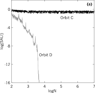
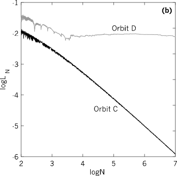
Figure 2: The evolution in log-log scale of (a) the SALI and (b) the finite time Lyapunov characteristic number $L_{N}$, with respect to the number $N$ of iterations of the 4D map (9) with $\nu=0.5$, $\kappa=0.1$, $\mu=10^{-3}$, for the ordered orbit C with initial condition $x_{1}=0.5$, $x_{2}=0$, $x_{3}=0.5$, $x_{4}=0$ (black line) and for the chaotic orbit D with initial condition $x_{1}=3$, $x_{2}=0$, $x_{3}=0.5$, $x_{4}=0$ (gray line).

In the case of the 4D map (9) for $\nu=0.5$, $\kappa=0.1$ and $\mu=10^{-3}$ we consider the ordered orbit C with initial condition $x_{1}=0.5$, $x_{2}=0$, $x_{3}=0.5$, $x_{4}=0$ and the chaotic orbit D with initial condition $x_{1}=3$, $x_{2}=0$, $x_{3}=0.5$, $x_{4}=0$. The initial deviation vectors used for the computation of the SALI are (1,1,1,1) and (1,0,0,0), for both orbits. As we see in figure 2(a) the SALI of the ordered orbit C remains almost constant (black line), fluctuating around $\mbox{SALI}\approx 0.28$. On the other hand, the SALI of the chaotic orbit D decreases abruptly, reaching the limit of accuracy of the computer ($10^{-16}$) after about $4.7\times 10^{3}$ iterations (gray line). After that time, the coordinates of the two vectors are represented by opposite numbers in the computer (since the SALI actually coincides with $d_{+}$ in this case), and any further computation of their evolution is not necessary. So, in 4D maps the SALI tends to zero for chaotic orbits, while it tends to a positive value for ordered orbits. Thus, the different behavior of SALI clearly distinguishes between ordered and chaotic motion. Another advantage of using the SALI is that we can be sure about the nature of the tested orbit faster than using LCN. This becomes evident by looking at the evolution of the finite time Lyapunov characteristic number $L_{N}$ (1) for orbits C and D in figure 2(b). As expected, for the ordered orbit C, $L_{N}$ decreases as the number of iterations $N$ increases, following a power law, reaching the value $L_{N}\approx 1.6\times 10^{-6}$ after $10^{7}$ iterations. On the other hand, $L_{N}$ of the chaotic orbit D, after some fluctuations, seems to stabilize near a constant non–zero value $L_{N}\approx 5\times 10^{-2}$ after $10^{7}$ iterations. By comparing panels (a) and (b) of figure 2 we see that, after about $4.7\times 10^{3}$ iterations we can be sure that orbit D is chaotic using the SALI, since it has become equal to $10^{-16}$ and the two deviation vectors practically coincide, while we cannot stop the computation of $L_{N}$ at that time, since it is not yet evident whether the LCN for orbit D will ultimately be zero or not.

3.2 The Hénon–Heiles Hamiltonian system

Figure 3: The Poincaré surface of section for $x=0$ of the two degrees of freedom Hénon–Heiles Hamiltonian (10) for H=1/8. The projection on the PSS of the initial conditions of the ordered orbit E ($x=0,\;y=0.55,\;p_{x}\simeq 0.2417,\;p_{y}=0$) and the chaotic orbit F ($x=0,\;y=-0.016,\;p_{x}\simeq 0.49974,\;p_{y}=0$) are marked by black and light-gray filled circles respectively. The axis $p_{y}=0$ is also plotted.

In order to illustrate the effectiveness of the SALI in determining chaotic vs. ordered orbits in Hamiltonian flows, we consider the two degrees of freedom Hénon–Heiles Hamiltonian [4]

$$H(x,y,p_{x},p_{y})=\frac{1}{2}(p_{x}^{2}+p_{y}^{2})+\frac{1}{2}(x^{2}+y^{2})+x^{2}y-\frac{1}{3}y^{3},$$ (10)

where $x$, $y$ are the generalized coordinates and $p_{x}$, $p_{y}$ the conjugate momenta. In particular, we consider the case of fixed energy $H=1/8$, for which the system exhibits a rich dynamical structure. As it can be seen on the Poincaré surface of section (PSS) for $x=0$ in figure 3 there exist islands of stability, where ordered motion occurs, as well as extensive regions where chaotic motion takes place.

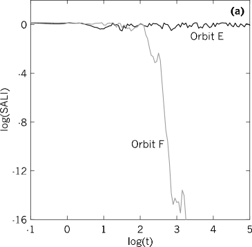
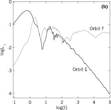
Figure 4: The evolution in log-log scale of (a) the SALI and (b) the finite time Lyapunov characteristic number $L_{t}$ as a function of time $t$, for the Hamiltonian (10) with H=1/8, for the ordered orbit E with initial condition $x=0,\;y=0.55,\;p_{x}\simeq 0.2417,\;p_{y}=0$ (black line) and for the chaotic orbit F with initial condition $x=0,\;y=-0.016,\;p_{x}\simeq 0.49974,\;p_{y}=0$ (gray line).

In order to apply the SALI method, we consider the ordered orbit E with initial condition $x=0,\;y=0.55,\;p_{x}\simeq 0.2417,\;p_{y}=0$ and the chaotic orbit F with initial condition $x=0,\;y=-0.016,\;p_{x}\simeq 0.49974,\;p_{y}=0$. The projection of the initial conditions of orbits E and F on the PSS are marked by black and light-gray filled circles respectively in figure 3. The initial deviation vectors $(dx(0),dy(0),dp_{x}(0),dp_{y}(0))$ used for the computation of SALI are $(1,0,0,0)$ and $(0,0,1,0)$. As we see in figure 4(a) the SALI of the ordered orbit E remains almost constant, fluctuating around $\mbox{SALI}\approx 1$ (black line), while the SALI of the chaotic orbit F decreases abruptly reaching the limit of accuracy of the computer $(10^{-16})$ after about 1,700 time units (gray line). The behavior of the SALI is similar to the one encountered in the 4D map (9) (figure 2(a)), since the phase space of the Hamiltonian system is 4–dimensional as in the case of the 4D map. In figure 4(b) we see the time evolution of finite time Lyapunov characteristic number $L_{t}$ (1) for orbits E (black line) and F (gray line). $L_{t}$ of the ordered orbit E, after an initial transient time interval where it exhibits large fluctuations, starts to decrease following a power law, reaching the value $L_{t}\approx 10^{-4}$ for $t=10^{5}$. $L_{t}$ of the chaotic orbit F has larger fluctuations without tending to zero, although even for $t=10^{5}$ it does not seem to stabilize around a non-zero value. We underline the fact that in this case, using the SALI we were absolutely sure that orbit F is chaotic at $t=1,700$, at which time SALI became practically zero, although at that time the use of $L_{t}$ could not give us the same information. In figure 3 we see that in a large portion of phase space the motion of system (10) is chaotic. The chaotic region corresponds to the area filled with scattered points on the PSS, while ordered motion corresponds to the islands formed by the invariant smooth curves. Since the SALI tends to completely different values for ordered and chaotic orbits, its computation for a sample of initial conditions can be used to distinguish between regions where ordered or chaotic motion occurs.

Figure 5: (a) The value of SALI for $t=4,000$ for orbits with initial conditions on the $p_{y}=0$ axis of the PSS shown in figure 3, as a function of the $y$ variable of the initial condition. The data are plotted as red points and are connected by blue lines. (b) Regions of different values of the SALI on the PSS $(y,p_{y})$ after 1,000 time steps. Initial conditions that give $\mbox{SALI}<10^{-12}$ are marked by black points, initial conditions that give $10^{-12}\leq\mbox{SALI}<10^{-8}$ are marked by deep blue points, initial conditions that give $10^{-8}\leq\mbox{SALI}<10^{-4}$ are marked by blue points, while initial conditions that give $10^{-4}\leq\mbox{SALI}$ are marked by light blue points.

As a first example, we consider orbits that lie on the $p_{y}=0$ line on the PSS shown in figure 3, having initial conditions $x=0$, $p_{y}=0$, while $p_{x}$ is defined by the Hamiltonian (10). The values of the SALI for all these orbits, after 4,000 time units, are plotted with red points in figure 5(a), as function of the $y$ variable of the initial condition. These points are line connected in order to be easily visible the changes of the SALI as the initial condition moves on the $p_{y}=0$ line. We can clearly see regions of ordered motion where the SALI has values larger than $10^{-4}$, corresponding to the islands of stability that are crossed by the line $p_{y}=0$ in figure 3. There also exist regions of chaotic motion where the SALI has become smaller than $10^{-12}$ or has even reached the limit of accuracy of the computer $(10^{-16})$, in agreement to the regions crossed by the $p_{y}=0$ line where scattered points exist on the PSS. Although most of the initial conditions give large $(\geq 10^{-4})$ or very small $(<10^{-12})$ values for the SALI, there also exist initial conditions that give, after 4,000 time units, intermediate values for the SALI $(10^{-12}\leq\mbox{SALI}<10^{-4})$. These correspond to sticky orbits existing near the borders of ordered motion, and more time is needed for the SALI to reach very small values and reveal their chaotic nature. By carrying out the above analysis not only on a line on the PSS but for the whole plane, plotting with different colors initial points that give values for the SALI in different ranges, we can get an image of phase space regions where ordered and chaotic motion are clearly distinguished (figure 5(b)). In figure 5(b) we see that our PSS is practically divided into regions where ordered motion occurs, colored in light blue, which corresponds to $10^{-4}\leq\mbox{SALI}$, and those colored in black, where chaotic behavior occurs, corresponding to $\mbox{SALI}<10^{-12}$. On the borders between these two regions we see points that give intermediate values for the SALI colored in deep blue ($10^{-12}\leq\mbox{SALI}<10^{-8}$) and in blue ($10^{-8}\leq\mbox{SALI}<10^{-4}$), which correspond to sticky orbits. The resemblance between figure 5(b) and figure 3 is obvious. We should also mention that in figure 5(b), we can see some very thin regions of ordered motion corresponding to very small islands of stability that cannot be seen easily in figure 3. So, it is evident that starting with any initial condition, the computed value of the SALI rapidly gives a clear view of chaotic vs. ordered motion even for systems described by ordinary differential equations, where surface of section plots are already time consuming for 2 degrees of freedom and practically useless for systems of higher dimensionality.

4 Conclusions

In this paper, we have given some examples of symplectic maps and Hamiltonian systems, where the computation of the smaller alignment index SALI allows us to distinguish in a cost effective way between ordered and chaotic orbits. The computation of the SALI is a fast, efficient and easy to compute numerical method, perfectly suited for multidimensional systems, but it can also be applied to 2D maps. In 2D maps, the SALI tends to zero both for ordered and chaotic orbits, but following completely different time rates which allows us to distinguish between the two cases. In maps of higher dimensionality (and Hamiltonian systems) the SALI tends to zero for chaotic orbits, while in general, it tends to a positive value for ordered orbits. So, we can easily distinguish between regular and chaotic orbits. Our approach, in fact, begins to be truly valuable for Hamiltonian systems of 2 degrees of freedom (where detailed surface of section plots are computationally too costly) and promises to become extremely useful for higher than 2 degree of freedom Hamiltonians and higher dimensional symplectic maps. An advantage of using the SALI in Hamiltonian systems or in multidimensional maps is that usually the chaotic nature of an orbit can be established beyond any doubt. This happens because when the orbit under consideration is chaotic, the SALI becomes zero, in the sense that it reaches the limit of the accuracy of the computer. After that time the two deviation vectors, needed for the computation of the SALI, are identical (equal or opposite), since their coordinates are represented by the same or opposite numbers. Thus, they have exactly the same evolution in time and cannot be separated. This practically means that we do not need to continue the computation of the evolution of the two vectors further on. We should also mention that in all cases studied, the use of the SALI helped us decide if an orbit is ordered or chaotic much faster than the computation of the finite time Lyapunov characteristic number $L_{t}$.

References

- [1] Benettin G., Galgani L. and Strelcyn J. M., 1976, Phys. Rev. A, 14, 2338
- [2] Froeschlé C., 1972, A&A, 16, 172
- [3] Froeschlé C., 1984, Celest. Mech., 34, 95
- [4] Hénon M., Heiles C., 1964, Astron. J., 69, 73
- [5] Skokos Ch., 2001, J. Phys. A, 34, 10029
- [6] Skokos Ch., Contopoulos G., Polymilis C., 1997, Celest. Mech. Dyn. Astron., 65, 223
- [7] Skokos Ch., Antonopoulos Ch., Bountis T. C. and Vrahatis M. N., 2002, in “CD-Rom Proceedings of GRACM 2002, 4th GRACM Congress on Computational Mechanics”, Univ. of Patras, Patras, Greece
- [8] Voglis N., Contopoulos G., Efthymiopoulos C., 1999, Celest. Mech. Dyn. Astron., 73, 211