The origin of diffusion: the case of non chaotic systems

Abstract

We investigate the origin of diffusion in non-chaotic systems. As an example, we consider $1$-$d$ map models whose slope is everywhere $1$ (therefore the Lyapunov exponent is zero) but with random quenched discontinuities and quasi-periodic forcing. The models are constructed as non-chaotic approximations of chaotic maps showing deterministic diffusion, and represent one-dimensional versions of a Lorentz gas with polygonal obstacles (e.g., the Ehrenfest wind tree model). In particular, a simple construction shows that these maps define non-chaotic billiards in space-time. The models exhibit, in a wide range of the parameters, the same diffusive behavior of the corresponding chaotic versions. We present evidence of two sufficient ingredients for diffusive behavior in one-dimensional, non-chaotic systems: i) a finite-size, algebraic instability mechanism, and ii) a mechanism that suppresses periodic orbits.

I Introduction

The presence of randomness in many natural processes is traditionally ascribed to the lack of perfect control on observations and experiments. Then, usually,“disorder” and “irregular behaviors” are considered only as unavoidable factors which, in phenomena modellizations, can be described effectively through external sources (random numbers in computer simulations, noise in stochastic equations etc.). However randomness may also have another origin associated to local instabilities of the deterministic microscopic dynamics of a system, i.e. microscopic chaos (MC). For instance, macroscopic diffusion of a particle in a fluid can be interpreted as a consequence of chaos on microscopic scales generated by collisions of the particle with the surrounding others.

The possibility of describing the Brownian behavior in terms of deterministic motion has stimulated a large amount of work in the field of deterministic diffusion to study purely deterministic systems exhibiting asymptotically a linear growth of the mean square displacement ChaoDiff ; ChaoDiff1 ; KD . The deterministic interpretation of transport phenomena establishes a close connection between transport and chaos theory, and, at least in principle, macroscopic properties such as transport coefficients (viscosity, thermal and electrical conductivity, diffusion etc.) could be directly computed through indicators of chaos GasNik ; Morriss ; Dorfman or by applying the standard techniques of chaos theory such as periodic orbit expansion Artuso ; Vance ; CEG95 ; Gaspard . However, considering randomness and transport in general as signatures of MC raises subtle and fundamental issues in statistical physics that have to be carefully discussed an investigated. First, there is the main problem of conceiving and realizing experiments able to prove, beyond any doubt, the existence of MC in real systems. An experiment in this direction was attempted in ref. Nature but the conclusions were object of criticism by many authors, as we discuss later. Besides, for real systems, the definition of MC appears to be ambiguous. Indeed, real systems involve a large number of degrees of freedom and their model description entails taking the thermodynamic limit but, in this limit, the concept of Lyapunov exponent becomes metric dependent so not well established GS . Moreover, the large number of degrees of freedom poses severe limitations also in the applicability of standard techniques to distinguish between chaotic and stochastic signals GP ; CP ; GW when data are extracted from real experiments. In fact, the noise-chaos distinction requires a extremely fine resolutions in the observations that is impossible to reach when one deals with systems with large dimensionality DCH ; DC ; Cencio .

References Nature ; Experiment summarized an ingenious experiment devised to infer the presence of chaos on microscopic scales. In the experiment the position of a Brownian particle in a fluid was recorded at regular time intervals. The time series were processed by using the same techniques developed for detecting chaos from data analysis CP ; GW . Authors measured a positive lower bound for the Kolmogorov-Sinai entropy, claiming that this was an experimental evidence for the presence of microscopic chaos. However in the papers  DCH and  DC it was argued that a similar result holds for a non-chaotic system too, hence the experiment cannot provide a conclusive evidence neither for the existence of microscopic chaos nor for the relevance of chaotic behavior in diffusion phenomena. Such papers shown that, through the analysis performed in Refs. Nature ; Experiment , there is no chance to observe differences in the diffusive behavior between a genuine deterministic chaotic systems as the 2-d Lorentz gas with circular obstacles Dorfman and its non chaotic variant: the wind-tree Ehrenfest model. The Ehrenfest model consists of free moving independent particles (wind) that scatter against square obstacles (trees) randomly distributed in the plane but with fixed orientation. Due to collisions, particles undergo diffusion, however their motion cannot be chaotic because a reflection by the flat planes of obstacles does not produce exponential trajectory separation; the divergence is at most algebraic leading to zero Lyapunov exponent. Such considerations can be extended to squares obstacles with random orientations and to every polygonal scatterers, so there is a whole class of models where diffusion occurs in the absence of chaotic motion. A difference between the 2-$d$ chaotic and non-chaotic Lorentz gas relies on the presence of periodic orbits DC .

The question that naturally arises “What is the microscopic origin of the diffusive behavior?” remains still open. In this paper, focusing on this problem, we extend the analysis of Dettman and Cohen showing that standard diffusion may also occur in one-dimensional models where every chaotic effect is surely absent. These systems, being one-dimensional, can be much easily studied than wind-tree models without spoiling the essence of the problem. Accurate results are obtained with relatively small computational efforts, and the interpretation of the results is clearer since we are able to better control and quantify the effects of the local instabilities. We shall see that, in such models, the relevant ingredients to obtain diffusion in the absence of deterministic chaos is the combined action of a “finite size instability”, quenched disorder and a quasi-periodic perturbation. Where by “finite size instability” we mean that infinitesimal perturbations are stable, while perturbations of finite size can grow algebraically. The interplay between these three features guarantees the system to be still diffusive as it would be chaotic. This outcome is another striking effect of finite size instabilities which make the behaviors of certain non-chaotic system similar, to some extent, to those generated by genuine chaotic systems (PLOK ; Cecconi ; Torcio ; LRB ). In ref. zasl the reader can find a study of an interesting system with weak mixing properties and zero Lyapunov exponent, i.e. an intermediate case between integrability and strong mixing.

The paper is organized as follows. In section II, we first recall the general features of $1$-$d$ models showing deterministic diffusion. Then we present two non-chaotic, one-dimensional models that exhibit deterministic diffusion when properly perturbed. In section III we characterize numerically the diffusion properties of the models and their dependence on the external perturbation. Section IV shows how these models can be viewed as non-chaotic space-time billiards, and discusses in more detail the role of periodic orbits. Section V is devoted to conclusions and remarks.

II Non-Chaotic Models for Deterministic Diffusion

Motivated by the problem of deterministic diffusion in non-chaotic Lorentz systems (i.e. with polygonal obstacles) we introduce models that, somehow, represent their one-dimensional analog. We begin considering one of the simplest chaotic model that generates deterministic diffusion: a $1$-$d$ discrete-time dynamical system on the real axis

$$x^{t+1}=[x^{t}]+F(x^{t}-[x^{t}])\,,$$ (1)

where $x^{t}$ is the variable performing the diffusion (position of a point-like particle) and $[\ldots]$ denotes the integer part. $F(u)$ is a map defined on the interval $[0,1]$ that fulfills the following properties

i)

$|F^{\prime}(u)|>1$, so the system has a positive Lyapunov exponent.

ii)

$F(u)$ must be larger than $1$ and smaller than $0$ for some values of $u$, so there exists a non vanishing probability to escape from each unit cell (a unit cell of real axis is every interval $C_{\ell}\equiv[\ell,\ell+1]$, with $\ell\in{\bf Z}$).

iii)

$F_{r}(u)=1-F_{l}(1-u)$, where $F_{l}$ and $F_{r}$ define the map in $u\in[0,1/2[$ and $u\in[1/2,1]$ respectively. This anti-symmetry condition with respect to $u=1/2$ is introduced to prevent the presence of a net drift.

The map, $u^{t+1}=F(u^{t})$ (mod $1$) is assumed to be also ergodic. One simple choice of $F$ is

$$F(u)=\left\{\begin{array}[]{ll}2(1+a)u\qquad\qquad\quad\,\,\mbox{if~{}}u\in[0,1/2[\\ 2(1+a)(u-1)+1\quad\mbox{if~{}}u\in[1/2,1]\end{array}\right.$$ (4)

where $a>0$ is the parameter controlling the instability. This model has been so widely studied, both analytically and numerically KD ; Klag ; Klag1 that can be considered as a reference model for deterministic diffusion. The deterministic chaos which governs the evolution inside each unit cell is responsible of the irregular jumping between cells and the overall dynamics appears diffusive, in the sense that asymptotically the variance of $x^{t}$ scales linearly with time. Following the literature on deterministic diffusion we consider systems with no net drift ($i.e.$ $\langle x^{t}\rangle/t\to 0$ for $t\to\infty$). In this paper we will see that there is no need to invoke chaos to induce diffusive behavior in 1-$d$ maps, as already shown in DC in the context of 2-$d$ billiards.

The construction of the models begins by dividing the first half of each unit cell $C_{\ell}$ into $N$ micro-intervals $[\ell+\xi_{n-1},\ell+\xi_{n}[$ , $n=1,\dots,N$, with $\xi_{0}=0<\xi_{1}<\xi_{2}<\dots<\xi_{N-1}<\xi_{N}=1/2$. In each micro-interval the maps are defined by prescribing a linear function $F_{\Delta}$ with unit slope. The map in the second half of the unit cell is determined by the anti-symmetry condition iii).

In the first model $\{\xi_{k}\}_{k=1}^{N-1}$ is a uniformly distributed random sequence between $[0,1/2]$, so the size of the micro-intervals is random and the function is defined as

$$F_{\Delta}(u)=\begin{array}[]{ll}u-\xi_{n}+F(\xi_{n})\qquad\quad\mbox{if~{}}u\in[\xi_{n-1},\xi_{n}[\;\;,\end{array}$$ (6)

where $F(\xi_{n})$ is the chaotic map function in Eq. (4) evaluated at $\xi_{n}$.

In the second model, the size of the micro-intervals is uniform, i.e. $|\xi_{n}-\xi_{n-1}|=1/N$, but the “height” of the function is random. That is,

$$F_{\Delta}(u)=\begin{array}[]{ll}u-\tilde{\xi}_{n}+\lambda_{n}\qquad\quad\mbox{if~{}}u\in[\xi_{n-1},\xi_{n}[\;\;,\end{array}$$ (8)

where $\tilde{\xi}=(\xi_{n-1}+\xi_{n})/2$, and the heigth at the mean point, $\lambda_{n}$, is a random variable distributed uniformly in the interval $[-\delta,1+\delta]$, with $\delta\geq 0$. Figures 1 and 2 show examples of these two models. Let us note that the random variables $\xi_{n}$ and $\lambda_{n}$ are quenched variables, i.e. in a given realization of a model they depend on the cell $C_{\ell}$ (so one should properly write $\xi_{n}^{(\ell)}$ and $\lambda_{n}^{(\ell)}$) but they do not depend on time.

As Fig. 1 illustrates in model (6) each cell is partitioned in the same number $N$ of randomly chosen micro-intervals of mean size $\Delta=1/N$ and in each of them the slope of the map (microscopic slope) is one. For $\Delta\to 0$ (equivalently $N\to\infty$) we recover the chaotic system (1) but the limit $F_{\Delta}\to F$ has to be carefully interpreted. This kind of modification of the original chaotic system is somehow equivalent to replacing circular by polygonal obstacles in the Lorentz system DC , since the steps with unitary slope are the analogous of the flat boundaries of the obstacles. The discontinuities of $F_{\Delta}$ produce a dispersion of trajectories in a way similar to that of a vertex of polygons that splits a narrow beam of particles hitting on it. However, at variance with the $2$-$d$ wind-tree model, both randomness and forcing are needed to attain a full diffusive behavior. Note that, thanks to the local preservation of the antisymmetry with respect to the cell center, no net drift is expected and also the Sinai-Golosov Sin ; Gol ; Quench effect is absent. Also model (8) is non-chaotic and the randomness is introduced in the function but not in the partition of the unit cells.

Since $F_{\Delta}$ has slope $1$ almost everywhere, the chaoticity condition i) is no more satisfied in these models. However, these models can exhibit diffusion provided condition i) is replaced by the following two requirements:

i-a)

presence of quenched disorder,

i-b)

presence of a quasi-periodic external perturbation.

In models (6) and (8), requirement i-a) is satisfied by the randomness in the partition of the micro-intervals, and the randomness in the linear function. To fulfill requirement i-b) we introduce a time-dependent perturbation into Eq. (1)

$$x^{t+1}=[x^{t}]+F_{\Delta}(x^{t}-[x^{t}])+\varepsilon\cos(\alpha t)$$ (9)

where $\varepsilon$ tunes the strength of the external forcing, $\alpha$ defines its frequency and the index $\Delta$ indicates a specific quenched disorder realization. We underline again that the linear piecewise map $F_{\Delta}$ explicitly depends on the cells $C_{\ell}$ due to the disorder, which varies from cell to cell.

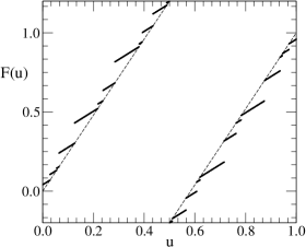
Figure 1: Sketch of the random staircase map in the unitary cell. The parameter $a$ defining the macroscopic slope is set to $0.23$. Half domain $[0,1/2]$ is divided into $N=12$ micro-intervals of random size. The map on $[1/2,1]$ is obtained by applying the antisymmetric transformation with respect to the center of the cell $(1/2,1/2)$

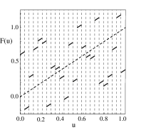
Figure 2: Sketch of model (8) in the unit cell. In this case the half domain $[0,1/2]$ is divided into $N=12$ uniform micro-intervals. The map on $[1/2,1]$ is obtained by applying the antisymmetric transformation with respect to the center of the cell $(1/2,1/2)$. In each micro-intervals the map is defined by prescribing a linear function with unit slope and random height, with $\delta=0.2$ (see text).

Even though by construction the system is not unstable in the Lyapunov sense, it exhibits standard diffusion. In particular, numerical simulations show a linear growth of the mean square displacement. It is important to note that, for model (6) a uniform partition of cell domains plus the quasi-periodic perturbation is not sufficient to produce diffusive dynamics. Even in the presence of quenched randomness (i.e. random partitions or random heights) alone, the system spontaneously settles onto periodic or quasi-periodic trajectories and does not diffuse. The periodic and quasi-periodic behavior is broken down, only when a time dependent perturbation is explicitly superimposed onto the quenched randomness. Hence, we can say that, in our models, the time plays somehow the role of the missing spatial dimension with respect to the $2$-$d$ models of ref. DC . We will explore this idea in more detail in Sec. V.

III Diffusion without chaos, numerical results.

In this section, we characterize the diffusion properties of model (6), while in the next, we discuss diffusion on model (8).

The diffusion coefficient,

$$D=\lim_{t\to\infty}\frac{1}{2t}\langle(x^{t}-x^{0})^{2}\rangle$$ (10)

has been numerically computed from the slope of the linear asymptotic behavior of the mean square displacement. The average has been performed over a large number of trajectories starting from random initial conditions uniformly distributed in cell $[0,1]$ and the results are shown in Fig. 3 for three different perturbation amplitudes $\varepsilon$. In all performed simultations we present in this section we set $\alpha=1$; the influence of $\alpha$ on diffusive behaviour is discussed in the following section.

We see that diffusion is absent for $\varepsilon$ small enough, thus, a transition between a diffusive to non-diffusive regime is expected upon decreasing $\varepsilon$.

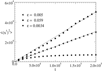
Figure 3: Time behavior of $\langle(x^{t})^{2}\rangle$ for three different perturbation amplitudes $\varepsilon$, $a=0.23$ and $N=100$ micro-intervals per cell.

When the limit in expression (10) exists, coefficient $D$ can be expressed in terms of the velocity correlation function as in Green-Kubo formula Dorfman ; Klag

$$D=\frac{1}{2}\langle(v^{0})^{2}\rangle+\sum_{k=1}^{\infty}\langle v^{0}v^{k}\rangle$$ (11)

where $x^{i+1}-x^{i}=v^{i}$ can be formally regarded as a discrete-time velocity. The simplest approximation for $D$ amounts to assuming that velocity correlations decay so fast that only the first term of the above series can be retained. In the pure chaotic system (1), this condition is often verified, and with the further assumption of uniform distribution for the quantity $x^{t}-[x^{t}]$, one obtains the approximated expression

$$D(a)=\frac{a}{2(1+a)}$$ (12)

that works rather well in the parameter region we explored Klag . In the non-chaotic system (9) this approximation is expected to hold only in the large driving regime limit, where the stair-wise structure of $F_{\Delta}$ is hidden by the perturbation effects.

The role of the external forcing on the activation of the diffusion process in the non chaotic system has been studied by looking at the behavior of the diffusion coefficient $D$ upon changing the perturbation amplitude $\varepsilon$ and the “discretization level” defined by the number of the micro-intervals $N$ in each cell.

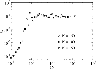
Figure 4: Log-Log plot of the dependence of the diffusion coefficient $D$ on the external forcing strength $\varepsilon$. Different data relative to a number of cell micro-intervals $N=50$, $100$ and $150$ are plotted vs the natural scaling variable $\varepsilon N$ to obtain a collapse of the curves. Horizontal line represents the theoretical result (12) holding for the chaotic system (1,4)

.

Results of Fig. 4 show that $D$ is significantly different from zero only for values $\varepsilon>\varepsilon_{c}$, for which the system performs normal diffusion. Below this threshold the values of $D$, when non zero, are so small that we cannot properly speak of diffusion. When $\varepsilon$ increases well above $\varepsilon_{c}$, $D$ exhibits a saturation toward the value predicted by formula (12) (horizontal line) for the chaotic system defined through (1,4). The onset of a diffusive regime as a threshold-like phenomenon, with respect to the external perturbation amplitude, is expected. It can be explained by noticing that, due to the staircase nature of the system, the perturbation has to exceed the typical discontinuity of $F_{\Delta}$, to activate the local instability which is the first step toward the diffusion. Data collapsing in Figs 4 confirms this view, because it is achieved by plotting $D$ versus the scaling variable $\varepsilon N$. This means that, for $N$ intervals on each cell, the typical discontinuity in the staircase-map is $O(1/N)$, then the $\varepsilon$-threshold is $\varepsilon_{c}\sim 1/N$. This behavior is robust and does not depend on the precise shape of the forcing, as we have verified by considering other kind of external perturbations. However, as will be discussed in the next section, there is some connection among the diffusive properties of the system, the periodic orbits, the parameter $N$, and the value of the perturbation frequency $\alpha$.

The activation of the instability performed by the perturbation can be studied by considering a well localized ensemble of initial conditions. We choose uniform initial distribution of ${\cal N}$ walkers with $\sigma_{0}^{2}\sim 10^{-12},10^{-8},10^{-6}$ and monitored the distribution spreading under the dynamics by following the evolution of its variance

$$\sigma^{2}(t)=\frac{1}{{\cal N}}\sum_{i=1}^{{\cal N}}\langle(x^{t}_{i}-\langle x^{t}_{i}\rangle)^{2}\rangle$$ (13)

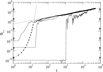
Figure 5: Time behavior of the variance (Eq. 13) for chaotic and non chaotic system with $a=0.23$. The discretization level is $N=100$ for the latter. Full lines refer to the non chaotic model and from below correspond to initial values $\sigma_{0}^{2}=10^{-12},10^{-8},10^{-6}$ respectively. For a direct comparison, full dots represent $\sigma^{2}(t)$ in the chaotic case, with $\sigma_{0}^{2}=10^{-12}$, which clearly exhibits a crossover from the exponential growth at small times (governed by Lyapunov exponent) to normal diffusion at large times. Dotted lines indicate the predicted chaotic growth $\exp(2\lambda t)$ and diffusion $2D(a)t$ (see formula 12).

Note that, in contrast with the average in Eq. (10) now the average is over an ensemble of initial conditions, uniformly distributed on a small size interval. The spreading of the initial cloud of points is better understood when we make a comparison between the chaotic (1) and non chaotic system (9). In the former, the instability makes the variance growing exponentially at the rate $\ln[2(1+a)]$ which is its Lyapunov exponent. This exponential separation lasts until the typical linear behavior of the diffusion takes place (see Fig. 5). In the non-chaotic system, instead, the behavior of $\sigma^{2}(t)$ strongly depends on its initial value $\sigma_{0}^{2}$ and we have to consider two sub-cases, whether $\sigma_{0}\gtrsim 1/N$ or $\sigma_{0}\ll 1/N$. When $\sigma_{0}\gtrsim 1/N$, basically one observes the same behavior of the continuous limit i.e. $\sigma^{2}(t)\sim\sigma_{0}^{2}\exp(2\lambda t)$ for times $t<t_{*}\sim\ln(1/\sigma_{0})$ and $\sigma^{2}(t)\sim t$ for $t>t_{*}$. Instead, if $\sigma_{0}\ll 1/N$ we can distinguish three different regimes: a) $\sigma(t)$ remains constant for a certain time span $[0,t_{1}]$, b) the instability starts being active and the $\sigma$ grows exponentially as in the chaotic case, $\sigma(t)\sim(1/N)\exp[\lambda(t-t_{1})]$, c) the system eventually reaches the regime of standard diffusion where $\sigma^{2}$ behaves linearly. The crossover time $t_{1}$ between the regimes a) and b) depends on the size of the discontinuities of $F_{\Delta}$ and the specific realization of the randomness and, of course, it decreases when either $N$ or $\sigma_{0}$ increases. We stress that the above scenario is due to the presence of finite size instabilities that in a non chaotic Lorentz gas would correspond to the defocusing mechanism of a beam by the vertices of polygonal obstacles.

The onset of standard diffusive behavior in model (9) depends on large-time features of the deterministic dynamics. Indeed the presence of periodic trajectories, standing or running note , have a strong influence on the diffusion, because the formers tend to suppress diffusion while the latter induce a “trivial” ballistic behavior. In Ref. DC , it has been conjectured that the main difference between a fully chaotic deterministic system and a non chaotic system exhibiting diffusion, as a consequence of quenched randomness, is in the different effects the periodic trajectories have on the systems. An escape rate method Dorfman ; Gaspard can be applied to analyze these effects. This method consists on starting with an ensemble of $W(0)$ trajectories initially localized in the region ${\cal R}_{L}$ between $-L/2$ and $L/2$ and computing the number $W(t)$ of them which never left ${\cal R}_{L}$ until the time $t$. For a pure random walk process one would expect an exponential decay

$$W(t)\sim\exp(-\gamma t)$$ (14)

where the rate $\gamma$ is proportional to the diffusion coefficient $D$ through the relation $\gamma\propto D/L^{2}$. In this sense the method is an alternative way to estimate the diffusion coefficient from measurement of $\gamma$. However possible deviations from (14) generally indicate a non diffusive behavior related to the presence of periodic orbits. As clearly seen in fig 6, on all the range of sizes $L$ we have considered, we do not observe any substantial deviation from the exponential decay that can be associated to periodic orbit effects.

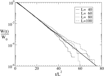
Figure 6: Exponential decay with time of the fraction $W(t)/W_{0}$ of walkers that, at time $t$, never left the region of length $L=40,60,80,100$, centered around the origin of the lattice of cells. Model parameters are $a=0.23$, $\varepsilon=0.1$ and $N=100$. The disorder configuration is replicated each $M=20$ cells. The walker are initially ($t=0$) placed inside the cell $[0,1]$

One can wonder whether the diffusive behavior could be merely due to a possible non zero spatial entropy per unit length of the quenched randomness. To unravel the role of static randomness as possible source of entropy and thus diffusion, following Ref. DC , we have considered a system were the same configuration of the disorder is repeated every $M$ cells (i.e. $\xi^{(\ell)}_{n}=\xi^{(\ell+M)}_{n}$), so the entropy for unit length is surely zero. This point is crucial, because, someone can argue that a deterministic infinite system with spatial randomness can be interpreted as an effective stochastic system, but this is a “matter of taste”. Anyway, our system with a spatially periodic randonness is deterministic from any point of view.

Looking at the diffusion of an ensemble of walkers we obtain that:

a)

there is weak average drift $V$, that vanishes approximately as $V\sim 1/M$ when $M$ goes to infinity.

b)

there is still a diffusive behavior i.e. $\langle(x^{t}-Vt)^{2}\rangle\sim 2Dt$, with a coefficient $D$ very close to the value obtained by formula (12).

Let us note that this behavior is obtained by considering single realizations of the randomness: the value of the drift changes with the realization, in such a way that an average on the disorder would give a null drift. The fact that $V\sim 1/M$ can be easily interpreted as a self-averaging property, for large $M$. On the other hand if we write $\langle(x^{t})^{2}\rangle=(Vt)^{2}+2Dt$, we can define a crossover time $\tau_{c}\sim DM^{2}$, from pure diffusive to a ballistic regime. When $M$ is finite but large enough the crossover time becomes very large. Therefore, we can safely conclude that, even with a vanishing (spatial) entropy density of randomness, at least for sufficiently large $M$, the system is able to effectively perform standard diffusion for a very long time. However we stress that looking at $\langle(x^{t}-Vt)^{2}\rangle$ we do not observe any crossover.

IV Space-time billiards

As mentioned previously, in the one-dimensional maps proposed in this paper, time plays the role of the second dimension in the two-dimensional billiard models (e.g., Lorentz and Ehrenfest models). Here we show this explicitly by describing how the one-dimensional time-dependent maps define billiards in space-time. For convenience, we carry out the construction for model (8) where the partition of the unit cells is uniform. However, the same construction can be done for model (6).

Let $[\xi_{n-1},\xi_{n}]$ be a micro-interval of a given unit cell. Then, for any initial condition $x_{0}\in[\xi_{n-1},\xi_{n}]$, the velocity of the particle at time $t$ is

$$h_{n}^{t}=x^{t+1}-x^{t}=\lambda_{n}+\varepsilon\,\cos(\alpha t)\,,$$ (15)

where $h_{n}^{t}$ is the height (including the time-dependent perturbation) of the piece-wise linear segment defining the map according to Eq. (8). As shown in Fig. 7, in a space-time diagram the “world-line” of this orbit is the straight line joining the points $(x^{t},t)=(x^{t+1},t+1)$ with slope $h_{n}^{t}$. Accordingly, as shown in Fig. 8, the space-time can be decomposed into discrete boxes $[\xi_{n-1},\xi_{n}]\times[t,t+1]$, and the world-line of successive iterates of the map appears as a zig-zag trajectory joining different boxes. The rule of the billiard is that a particle entering box $n$ will leave this box with speed $h^{t}_{n}$. That is, in going from box $m$ to box $n$ a particle suffers a space-time scattering event $\delta v=h^{t+1}_{n}-h^{t}_{m}$, where $\delta v=v^{t+1}-v^{t}$ is the change in the particle velocity. In the space-time diagram the scattering rule is represented by drawing at each box a line segment with slope given by $h^{t}_{n}$ that according to (15) has a random component $\lambda_{n}$, and a time-periodic component.

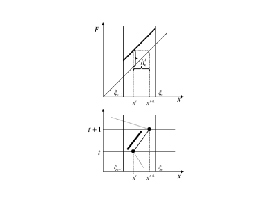
Figure 7: Construction of space-time billiard from a piece-wise linear with unit slope map.

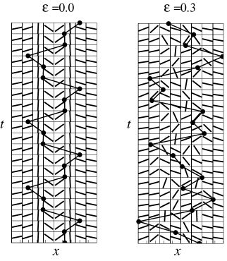
Figure 8: Space-time billiards without time dependence ($\varepsilon=0$), and with time dependence ($\varepsilon\neq 0$).

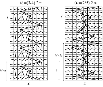
Figure 9: Periodic orbits in a space-time billiard with rational perturbation frequency

.

According to this, the time-dependent, zero-Lyapunov exponent (slope one) map is equivalent to a space-time billiard with scattering rule $h^{t}_{n}$. Note that these models are simpler than the usual 2-$d$ billiards (e.g. Lorentz gas) because the scattering rule is independent of the angle of incidence. Although this is just a reformulation of the same model, the billiard construction provides useful insights into the problem and allows the connection with the two-dimensional billiard problems. When the map is time-independent ($\varepsilon=0$) the scattering rule depends only on $n$ ($h_{n}^{p}=h_{n}^{q}$ for any integers $p$ and $q$) and as shown in Fig. 8-(a) the billiard structure is simply a copy of the billiard at $t=0$. In this case, despite the spatial randomness, the lack of a time dependence leads to a highly structured space-time billiard in which periodic orbits are ubiquitous. As a consequence, in this case there is no diffusion, a result already mentioned before. On the other hand, as Figure 8-(b) shows, when $\varepsilon\neq 0$ the billiard exhibits space-time disorder which leads to the possibility of diffusive behavior.

As discussed in Ref. DC for polygonal two-dimensional billiards, periodic orbits play an important role. The existence of periodic orbits in the space-time billiard is intimately connected with the frequency $\alpha$ of the time periodic perturbation. If $\{x^{t}\}$ is a periodic orbit of period $M$ ($x^{t+M}=x^{t}$ for any $t$), the billiard must be $q$-periodic, that is $h_{n}^{t+q}=h_{n}^{t}$ for any $t$, where $M=mq$ and $m$ is a positive integer. According to Eq. (15) this will be the case provided

$$\alpha=2\,\pi\,\nu\,,$$ (16)

with $\nu=p/q$. Figure 9 show two examples of periodic orbits with $\varepsilon=0.2$. In panel (a), $\alpha=2\pi(3/4)$, and the period of the billiard is the same as the period of the orbit, $q=M=4$. In panel (b), $\alpha=2\pi(2/5)$, and the period of the orbit is twice period of the billiard $M=2q=10$. Thus, for rational $\nu$ the billiard shows a periodic structure in time, and periodic orbits are likely to exist leading to the suppression of diffusion. On the other hand, when $\nu$ is an irrational number the billiard structure never repeats exactly in time and strictly speaking there are no periodic orbits. Motivated by this, it is possible to related the degree of temporal disorder of the billiard to the degree of irrationality of $\nu$ as determined, for example, by the continued fraction approximation of $\nu$. In this regard, billiards with irrational frequencies $\nu$ which are easily approximated by rationals are “less disordered” than billiards with hard to approximate frequencies. To explore this ideas Fig. 10 shows the time evolution of the variance for different values of the perturbation frequency in the same random realization of model (8) with $N=40$ and $\varepsilon=0.4$. For the perturbation frequencies, $\alpha=(p/q)2\pi$, we took the continued fraction expansion of the inverse golden mean

$$\nu=1/2,\,2/3,\,3/5,\,\ldots F_{n-1}/F_{n}\,\ldots\rightarrow\left(\sqrt{5}-1\right)/2=\gamma^{-1},$$ (17)

where $F_{0}=F_{1}=1$, and $F_{n}=F_{n-1}+F_{n-2}$. The chose of the golden mean is motivated by the fact that this number is the hardest to approximate with rational. In the model the disorder configuration is repeated every $M$ cells, and for small $M$ the recurrence time of an orbit (i.e. the time to return to the same microinterval, module $M$) decreases. Since we are interested in the role of periodic orbits, here we consider the limit case $M=1$. That is, in the simulations reported in Fig. 10, the disorder configuration in the unit interval $[0,1]$ was copied to all the cells $[\ell,\ell+1]$. As expected the figure shows the suppression of diffusion for rational frequencies. However, more interesting is the fact that there is a tendency for the onset of the suppression of diffusion to increase as $\nu$ approaches $1/\gamma$. This is related to the fact that for rationals with lower denominators the time period of the billiard is small, and the probability that the recurrence time of an orbit coincides with a multiple of the period of the billiard is high. The recurrence time is also related to the value of $N$. When $N$ is large, the probability for an initial condition to return to the same micro-interval (module $M$) is small, and periodic orbits are more scarce. This explains why for large enough $N$ and $M$, diffusion might not be suppressed even for rational frequencies with large denominators. This suggests that, for large enough $N$ and $M$, deviations from diffusion are unlikely to be observed numerically in the case of rational frequencies with large denominators.

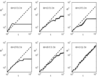
Figure 10: Mean square displacement as function of time in model (8) for a sequence of values of the perturbation frequency $\alpha$ approaching the inverse golden mean $1/\gamma$. The heights of map are uniformely distributed in $[0,1]$ ($\delta=0$ see text).

V Conclusions and remarks

From the above results we can conclude that two basic ingredients are relevant for diffusion, 1) a finite size instability mechanism: in the chaotic system this is given by the Lyapunov instability, in the ”stepwise” system this effect stems from the jumps 2) a mechanism to suppress periodic orbits and therefore to allow for a diffusion at large scales. In the presence of “strong chaos” (i.e. when all the periodic orbits are unstable) point 2) is automatically guaranteed thus the periodic orbits formalism Artuso ; CEG95 ; Dorfman can be fully applied to compute the diffusion coefficient. In non chaotic systems, however, like the present one, the mechanism 2) is the result of a combined effect of quenched randomness and quasi-periodic forcing.

In summary, we have introduced and studied models exhibiting diffusion in the absence of any source of chaotic behavior. The models represent the $1$-$d$ analogue of non chaotic Lorentz gas (i.e. with polygonal obstacles) discussed by other authors in connection with the debate around experimental evidences for a distinction between chaotic and stochastic diffusion. Our results indicate that when the chaotic instability condition (positive Lyapunov exponent) is replaced by the presence of finite size instability (non positive Lyapunov exponent) we need both an external quasi-periodic perturbation and disorder for preventing the system falling into either a periodic/quasi-periodic evolution or a drift dominated behavior.

We believe that this kind of behaviour is rather general, in the sense that chaos does not seem to be a necessary condition for the validity of some statistical features. This is in agreement with the recent results of Ref. LRB , where the applicability of the generalized Gallavotti-Cohen fluctuation formula GC has been proven for non chaotic systems too.

VI Acknowledgments

This work has been partially supported by MIUR (Cofin. Fisica Statistica di Sistemi Classici e Quantistici). D dCN was supported by the Oak Ridge National Laboratory, managed by UT-Battelle, LLC, for the U.S. Department of Energy under Contract No. DE-AC05-00OR22725. We thank Massimo Cencini and Stefano Ruffo for useful suggestions and discussions. D dCN gratefully acknowledges the hospitality of the Department of Physics of the University of Rome “La Sapienza” during the elaboration of this work.

References

- (1) S. Grossmann and H. Fujisaka, Phys. Rev. A 26 (1982) 1179.
- (2) T. Geisel and J. Nierwetberg, Phys. Rev. Lett. 26 (1982) 7.
- (3) R. Klages and R. Dorfman, Phys. Rev. Lett. 74 (1995) 387.
- (4) P. Gaspard and G. Nicolis, Phys. Rev. Lett (1990) 65 1693.
- (5) D.J. Evans and G.P. Morriss “Statistical Mechanics of non Equilibrium Fluids” (Academic-Press, London 1990.)
- (6) J.R. Dorfman “An Introduction to Chaos in Non Equilibrium Statistical Mechanics” (Cambridge University Press, Cambridge 1999).
- (7) R. Artuso, Phys. Lett. A (1991) 160 528.
- (8) W.N. Vance,Phys. Rev. Lett., 96 (1992) 1356.
- (9) P. Cvitanovic, J.P. Eckmann and P. Gaspard, Chaos, Solitons and Fractals 2 (1995) 113.
- (10) P. Gaspard “Chaos Scattering and Statistical Mechanics” (Cambridge University Press, Cambridge 1998).
- (11) P. Gaspard, M.E. Briggs, M.K. Francis, J.V. Sengers, R.W. Gammon, J.R. Dorfman and R.V. Calabrese, Nature, 394 (1998) 865.
- (12) P. Grassberger and T. Schreiber, Nature 401 (1999) 876.
- (13) P. Grassberger and I. Procaccia, Phys. Rev. A 28 (1983) 2591.
- (14) A. Cohen and I. Procaccia, Phys. Rev. A 31 (1985) 1872.
- (15) P. Gaspard and X.J. Wang, Phys. Report 235 (1993) 291.
- (16) C.P. Dettmann, E.D.G. Cohen and H. van Beijeren, Nature 401 (1999) 875.
- (17) C.P. Dettmann and E.D.G. Cohen, J. Stat. Phys. 101 (2000) 775.
- (18) M. Cencini, M. Falcioni, E. Olbrich, H. Kantz and A. Vulpiani Phys. Rev. E 62 (2000) 427.
- (19) M.E. Briggs, J.V. Sengers, M.K. Francis, P. Gaspard, R.W. Gammon and J.R. Dorfman, Physica A 296 (2001) 42.
- (20) A. Politi, R. Livi, G.L. Oppo and R. Kapral, Europhys. Lett. 22 (1993) 571.
- (21) F. Cecconi, R. Livi and A. Politi, Phys. Rev. E 57 (1998) 2703.
- (22) M. Cencini and A. Torcini, Phys. Rev. E 63 (2001) 056201.
- (23) S. Lepri, L. Rondoni and G. Benettin, J. Stat. Phys. 99 (2000) 857.
- (24) G.M. Zaslawsky and M. Edelman, Chaos 11 (2001) 295.
- (25) R. Klages and N. Korabel, J.Phys.A: Math.Gen. 35 (2002) 4823.
- (26) R. Klages, Phys. Rev. E 65 (2002) 055203(R).
- (27) Ya.G. Sinai, Theory Prob. Appl. 27 (1982) 256.
- (28) A. Golosov, Commun. Math. Phys. 92 (1984) 491.
- (29) G. Radons, Phys. Rev. Lett. 77, (1996) 4748.
- (30) A periodic trajectory , of period , is called standing when we have , while is called running when , being an integer indicating the lattice traslation.
- (31) G. Gallavotti and E.G.D Cohen., Phys. Rev. Lett. 74, (1995) 2694.