Path integration over closed loops and Gutzwiller’s trace formula

Abstract

In $1967$ M.C. Gutzwiller succeeded to derive the semiclassical expression of the quantum energy density of systems exhibiting a chaotic Hamiltonian dynamics in the classical limit. The result is known as the Gutzwiller trace formula.

The scope of this review is to present in a self-contained way recent developments in functional determinant theory allowing to revisit the Gutzwiller trace formula in the spirit of field theory.

The field theoretic setup permits to work explicitly at every step of the derivation of the trace formula with invariant quantities of classical periodic orbits. R. Forman’s theory of functional determinants of linear, non singular elliptic operators yields the expression of quantum quadratic fluctuations around classical periodic orbits directly in terms of the monodromy matrix of the periodic orbits.

The phase factor associated to quadratic fluctuations, the Maslov phase, is shown to be specified by the Morse index for closed extremals, also known as Conley and Zehnder index.

Introduction

The Gutzwiller trace formula is the semiclassical expression of the energy density of a quantum system [81, 82, 83, 84, 87, 88]. Despite of the mathematical difficulties with which it is intertwined, it represents the cornerstone of the present understanding of the manifestations of the quasi-stochastic nature of the trajectories of a generic, chaotic, classical system in the properties of the quantum mechanics associated to it by Bohr’s correspondence principle.

The trace formula states that the energy spectrum of a non relativistic quantum system is given by a series over all the periodic orbit of the classical system. The discovery of the trace formula revived the intuition of Bohr and Sommerfeld [28, 148] in the early days of quantum theory that the energy spectrum of a generic quantum system can be expressed in terms of the invariant properties of the periodic orbits of the corresponding classical system. The derivation of the trace formula is highly non trivial due to the singular nature of the classical limit of quantum mechanics.
Feynman’s path integrals offer the physically most transparent route to take the limit. Indeed path integrals were the starting point of Gutzwiller’s analysis. At the same time, the very discovery in the late sixties of the trace formula corresponded also to a major progress in the understanding of real time path integration. Namely Gutzwiller realised that the known Van Vleck-Pauli-Morette [117, 127, 155] approximation of the semiclassical propagator had to be corrected by the introduction of a further phase factor in correspondence of conjugate points of the classical trajectory. The phase factor turned out to be specified by the Morse index for open extremals [118]. The occurrence of the Morse index in the semiclassical propagator is experimentally observable. Namely, the phase of the propagator enters the Bohr-Sommerfeld quantisation condition and its generalisations as they emerge from the trace formula.
The role and significance of the propagator phase were further clarified by the ensuing fundamental investigations of the semiclassical limit carried out by Maslov [109], Voros [158] and Miller [111].

The works of Gutzwiller and Maslov laid also the basis for the development of functional semiclassical methods in field theory. Gutzwiller’s idea to compute atomic spectra without resorting to the construction of wave functions is of great advantage in field theory where state functionals are exceedingly complicated objects. Dashen, Hasslacher and Neveu [43, 44, 45] used the trace formula as a paradigm in their ground-breaking investigations of particle spectra of field theories.
Since the second half of the seventies the kinds of semiclassical approximations underlying the trace formula became familiar tools of theoretical physics. Among the early applications one can mention the monopole quantisation in the Georgi-Glashow model by ’t Hooft [152] and Polyakov [130] and the development the instanton formalism of Belavin, Polyakov, Schwartz and Tyupkin [17] and ’t Hooft [153].

The semiclassical approximation of path integrals is an infinite dimensional implementation of stationary phase methods. Fluctuations around the field configuration dominating the path integral in the semiclassical limit are, within leading order, generically quadratic. The resulting infinite dimensional Fresnel integral brings about the exigency of computing the square root of the determinant of the self-adjoint operator governing the quadratic fluctuations. Thus, a natural mathematical counterpart of path integral semiclassical methods is the theory of functional determinants.
Non-relativistic systems with strictly positive definite kinetic energy offer an intuitive framework to understand the mathematical issues interwoven with the evaluation of functional determinants. Since the quantum dynamics can be described by means of configuration space path integrals, the self-adjoint fluctuation operators emerging in the semiclassical approximation are of Sturm-Liouville type with spectrum bounded from below. The finite number of negative eigenvalues, the Morse index, by fixing the value of the phase of the quadratic path integral, provides a natural definition of the winding number of the functional determinant in the complex plane.
An intrinsic interpretation of the result is achieved by embedding the fluctuation operator in a family the elements of which are related by homotopy transformations. Thus, the phase of the functional determinant is specified by the winding number of the determinant bundle obtained by connecting the elements of the family to a positive definite operator with zero Morse index. Homotopy transformations may clip the explicit form of the operator as well as the boundary conditions obeyed by its functional domain of definition. A satisfactory theory should then be able to resolve the dependence of functional determinants versus the parameters entering the operator and the boundary conditions. A powerful result was recently obtained by R. Forman [67] for functional determinants of a rather general class of elliptic operators. In the context of non-relativistic quantum mechanics Forman’s result allows a particularly compact and intuitive expression of the semiclassical approximation of path integrals with general boundary conditions. The result has the further merit to provide a topological characterisation of extremals of classical mechanical action functionals independently of the adoption of a Lagrangian or Hamiltonian formalism. In consequence of Forman’s result, it is possible to establish the equality of the functional determinants of the self-adjoint operators associated to the second variation around a classical trajectory in configuration and phase space. In this latter case quadratic fluctuations are governed by Dirac type operators the spectrum whereof is unbounded from below and from above. The proof of index theorems for such Dirac operators is based on the construction of an infinite dimensional Morse theory ultimately relying on spectral (Fredholm) flow theorems (see [137, 143] and references therein; the particular case of open extremals was previously studied in the physical literature in [101, 103, 114] ). In the periodic case, the resulting index is named in the mathematical literature after Conley and Zehnder who showed its role in the proof of existence statements for periodic solutions of time periodic and asymptotically linear Hamiltonians [35]. The equality of the functional determinants entails immediately that the Conley and Zehnder index coincides with the Morse index for closed extremals whenever both of them are defined. The result is proven in the mathematical literature by different, less intuitive methods [3]. In the physical literature an equivalent result was obtained by Sugita in [150].

The modern theory of functional determinant provides considerable insight in the Gutzwiller trace formula.
In the traditional derivation the resort to path integration is restricted to the construction of the quantum propagator. This is equivalent to applying functional determinant theory only to fluctuation operators with Dirichlet boundary conditions exploiting a classical result of Gel’fand and Yaglom [72]. The semiclassical trace operation is carried out in a separate step. The re-parametrisation invariance [130] of closed quantum paths contributing to the density of states is broken in the process of the stationary phase approximation. In consequence, classical periodic orbits do not appear at intermediate steps. They are shown to fully characterise the final result only after nontrivial algebraic manipulations which require a good deal of a priori physical insight. More seriously the canonical invariance of the trace, although physically expected, needs to be proven apart. The proof relies on an highly non trivial mathematical apparatus developed by Arnol’d [8] and investigated in the physical literature by Littlejohn, Creagh and Robbins [39, 105, 140].
The situation is much simpler if the stationary phase approximation is carried out directly on the loop space where trace path integrals have support. Periodic functional determinants completely specify the contribution of quadratic fluctuations. The topological invariance of the phase factors is guaranteed by the Morse index theory for closed extremals [118]. The topological formulation of Morse index theory of Bott [29] and Duistermaat [56, 40] renders then a priori available an arbitrary number of equivalent prescriptions for the explicit evaluation of the index.

The aim of the present report is to review at a level as elementary as possible the general mathematical methods needed for a pure path integral derivation of the Gutzwiller trace formula. The systematic application of these methods to the energy density of a non relativistic quantum system in the semiclassical limit is itself a novelty. The merits of the path integral formulation are particularly evident when the Lagrangian of the classical system is invariant under extra continuous symmetries beyond time translations. In the path integral formalism, such situations present no conceptual difference from the case when the energy is the only conserved quantity. In all cases trace path integrals are handled in a canonically invariant way by means of the Faddeev-Popov method [60, 61].

The report is organised as follows. In chapter 1 the definition of the quantum density of states is recalled. The expression of the semiclassical approximation found by Gutzwiller is then qualitatively discussed. Chapter 2 focuses on functional determinant theory and Forman’s identity. Since the motivation is the semiclassical approximation of path integrals, the probabilistic interpretation of these latter ones is recalled in the first section of the chapter. Further details together with an outline of the recent rigorous proof [5] of the existence of the covariant representation of the path integral measure are given in appendix C. Chapter 3 summarises basic results of Morse index theory [118, 112]. The goal is to motivate the use of the symplectic geometry and differential topology concepts applied in the modern formulation of the theory [56, 40, 143, 4] and to emphasise their physical relevance. The theory is illustrated with examples. Finally, it is shown how to derive from the general formalism practical prescriptions to compute the phase factors intervening in the Gutzwiller trace formula. Chapter 4, the last, deals with implementation of the Faddeev-Popov method for trace path integrals. The Gutzwiller trace formula is then proven to follow immediately from the application of the method.
The material is expounded in each chapter in an as far as possible self-consistent way in order to allow independent reading. The main text is complemented by appendices summarising basic concepts of stochastic calculus and classical mechanics.

The author’s wish is that this may serve the reader interested not only in the Gutzwiller trace formula but also in understanding methods of path integration of general use in theoretical physics.

1 The density of states in quantum mechanics

The aim of the present chapter is to set the scene for the path integral methods which will be illustrated in the rest of this work. Some basic concepts of non relativistic quantum dynamics are shortly recalled in order to derive the relation between the density of states and the propagator. The relation is the starting point for the semiclassical approximations which led Gutzwiller to write his trace formula. Finally, the qualitative features and the significance for quantum mechanics of the trace formula are shortly discussed.

1.1 From the Schrödinger equation to the energy density

Non relativistic quantum mechanics for a spin-less particle is governed by the Schrödinger equation

$$i\,\hbar\,\partial_{T}\psi-H\,\psi=0$$

(1)

where $\psi$ is the wave function, $H$ the Hamiltonian operator and $\hbar$ Planck’s constant. This latter is a pure number if absolute units are adopted

$$[\,P\,]\,=\,-\,[\,Q\,]\,=\,1$$ (2)

$Q$ and $P$ being respectively the spatial position and the canonically conjugated momentum variables. The wave function $\psi$ is in general a complex valued function. It specifies the probability amplitude to observe the system in the position $Q$ at time $T$: the modulus squared $|\psi|^{2}$ defines the probability density of the same event (see for example [53, 64, 98, 141]).
In typical situations a quantum particle of mass $m$ interacts with an external potential $U$ and with a vector potential $A_{\alpha}$. Most often the physical configuration space $\mathfrak{M}$ is modeled by the Euclidean space $\mathbb{R}^{d}$, eventually represented in non Cartesian coordinates. A slight generalisation is to imagine $\mathfrak{M}$ to be a Riemann manifold which is either compact or $\mathbb{R}^{d}$ and has time independent metric $g_{\alpha\,\beta}$. In such a case the Hamilton operator is

$$H\,\psi\,:=\,\frac{1}{2}\,g^{\alpha\,\beta}\frac{(P_{\alpha}+A_{\alpha})\,(P_{\beta}+A_{\beta})}{m}\,\psi+U\,\psi$$ (3)

where $A_{\alpha}$ and $U$ are functions of $Q$ and eventually $T$ and $g^{\alpha\,\beta}$ is the inverse of $g_{\alpha\,\beta}$. In (3) the $P_{\alpha}$’s denote momentum operators in position representation. They act on all objects to their right as covariant derivatives

$$P_{\alpha}:=-i\,\hbar\,\nabla_{\alpha}$$ (4)

and therefore they obey the Leibniz rule

$$P_{\alpha}A^{\alpha}\psi=(P_{\alpha}A^{\alpha})\psi+A^{\alpha}P_{\alpha}\psi$$ (5)

The explicit form of the covariant derivative is fixed by the compatibility condition with the metric assigned to $\mathfrak{M}$. These geometric concepts are recalled in appendix A.
The Hamilton operator acts on the space $\mathbb{L}^{2}_{\mathfrak{M}}$ of square integrable functions on $\mathfrak{M}$ such that the Schrödinger equation is self-adjoint with respect to the scalar product

$$\langle\varphi\,,\psi\rangle\,=\,\int_{\mathfrak{M}}d^{d}Q\sqrt{g(Q)}\,(\varphi^{*}\psi)(Q,T)$$

$$g:=\det\{g_{\alpha\,\beta}\}$$ (6)

If the potentials $A_{\alpha}$ and $U$ are time independent it is possible to introduce the stationary Schrödinger equation

$$E\,\psi_{E}-H\,\psi_{E}=0$$ (7)

describing a quantum phenomenon occurring at a constant energy $E$. For bounded physical systems, the stationary equation admits solutions only if the energy assumes discrete, quantised, values. The energy levels are in such a case labelled by a set of integers referred to as quantum numbers.

The imaginary factor appearing in the Schrödinger equation (1) ensures invariance under time reversal of the dynamics of isolated quantum systems. Nevertheless it is useful to introduce the forward time evolution operator or propagator. The kernel $K$ of the propagator is specified by the solution of

$$\begin{array}[]{ll}(i\,\hbar\,\partial_{T}-H)K(Q,T|Q^{\prime},T^{\prime})=-i\,\delta(T-T^{\prime})\delta(Q-Q^{\prime})\,,&\quad T\,\geq\,T^{\prime}\\ K(Q,T|Q^{\prime},T^{\prime})=0\,,&\quad T\,<\,T^{\prime}\end{array}$$ (10)

The propagator is the inverse of the Hamilton operator for Cauchy boundary conditions in time. The propagator owns its name because it governs the propagation forward in time of wave functions

$$\psi(Q,T)=\int_{\mathfrak{M}}d^{d}Q^{\prime}\sqrt{g(Q^{\prime})}\,K(Q,T|Q^{\prime},T^{\prime})\,\psi(Q^{\prime},T^{\prime})$$ (11)

If the Hamiltonian is time independent and the energy spectrum discrete the propagator is amenable in the sense of $\mathbb{L}^{2}_{\mathfrak{M}}$ to a series over the eigenfunctions of the stationary Hamilton equation

$$K(Q,T|Q^{\prime},T^{\prime})=\theta(T-T^{\prime})\,\sum_{n}\,\psi_{n}(Q)\,\psi_{n}^{*}(Q^{\prime})\,e^{-i\,\frac{E_{n}\,(T-T^{\prime})}{\hbar}}$$ (12)

where $\theta(T-T^{\prime})$ is the Heaviside step function

$$\theta(T-T^{\prime})=\left\{\begin{array}[]{lll}1&\quad\mathrm{if}&T\,\geq\,T^{\prime}\\ 0&\quad\mathrm{if}&T\,<\,T^{\prime}\end{array}\right.$$ (15)

Analogous representations exist for continuous and mixed spectra.

The energy spectrum of the quantum system can be computed from the Fourier-Laplace transform of the propagator. The latter is given by the analytic continuation in the upper complex energy-plane

$$\int_{0}^{\infty}\frac{dT}{\hbar}\,e^{i\,\frac{Z\,T}{\hbar}}\,K(Q,T|Q^{\prime},0)=i\,\sum_{n}\,\frac{\psi_{n}(Q)\,\psi_{n}^{+}(Q^{\prime})}{Z-E_{n}}:=i\,G(Q|Q^{\prime},E)$$

$$Z\in\mathbb{C}\,,\quad\mathrm{Im}Z\,>\,0$$ (16)

The result is proportional to the kernel of the Green function $G$, the resolvent of the time independent problem

$$(Z\,-H)G(Q|Q^{\prime},Z)=\delta(Q-Q^{\prime})\,,\quad\quad\mathrm{Im}\,Z\,>0$$

$$G(Q|Q^{\prime},Z)=\int_{0}^{\infty}\frac{dT}{i\,\hbar}\,e^{i\,\frac{Z\,T}{\hbar}}\,K(Q,T|Q^{\prime},0)$$ (17)

The poles of $G$ are located on the real axis and coincide with the energy levels of the quantum system. Using the Plemelj identity [162]

$$\left.\lim_{\mathrm{Im}\,Z\,\downarrow 0}\frac{1}{Z-E_{n}}\right|_{E=\mathrm{Re}\,Z}=\mathrm{P.V.}\frac{1}{E-E_{n}}-i\,\pi\,\delta(E-E_{n})$$ (18)

where $\mathrm{P.V.}$ denotes the integral principal value, the announced relation between the energy density of the system and the trace of $G$ is found

$$\rho(E)=-\left.\lim_{\mathrm{Im}\,Z\,\downarrow 0}\,\mathrm{Im}\frac{1}{\pi}\int_{\mathfrak{M}}d^{d}Q\,\sqrt{g(Q)}G(Q|Q,Z)\right|_{E=\mathrm{Re}\,Z}$$ (19)

Physically (19) means that the energy density is a scalar quantity in non-relativistic Quantum Mechanics, independent of the representation of the Hilbert space.

Finally, in terms of the propagator the energy density reads

$$\rho(E)=-\left.\lim_{\mathrm{Im}\,Z\,\downarrow 0}\,\mathrm{Im}\,\int_{0}^{\infty}\frac{dT}{i\,\pi\,\hbar}\,e^{i\,\frac{Z\,T}{\hbar}}\,\int_{\mathfrak{M}}d^{d}Q\sqrt{g(Q)}\,K(Q,T|Q,0)\right|_{E=\mathrm{Re}\,Z}$$ (20)

1.2 The semiclassical limit and the Gutzwiller trace formula

The relation between the trace of the propagator and the energy density provides a way to extract information on the spectrum of a quantum system without solving the stationary Schrödinger equation (7). Indeed the propagator can be regarded as a more fundamental object than the Schrödinger equation. According to Feynman’s formulation of quantum mechanics [62, 64] the propagator is the “sum”

$$K(Q,T|Q^{\prime},T^{\prime})\,\thicksim\,\mbox{``}\sum_{\mathrm{paths}}\,e^{i\,\frac{\mathcal{S}(\mathrm{path})}{\hbar}}\,\mbox{''}$$ (21)

extended over all paths in configuration space connecting $Q$ to $Q^{\prime}$ in the time interval $[T^{\prime},T]$. Each path contributes with a phase specified by the action functional $\mathcal{S}$. The precise meaning of the sum will be recalled later. Here it is interesting to observe that classical mechanics is recovered in the singular limit of $\hbar$ tending to zero. The limit is directly meaningful in absolute units. In general units it will correspond to the vanishing of an overall adimensional parameter obtained from the Planck constant times other invariant quantities of the physical system.
Bohr’s correspondence principle requires the recovery of classical mechanics when $\hbar$ tends to zero while all the other parameters are held fixed. The existence of the limit entails the possibility to investigate a range of phenomena for which quantum effects are weak by means of an asymptotic expansion around the classical limit, the semiclassical expansion.

Broadly speaking the semiclassical approximation is expected to apply to the description of phenomena occurring at energy scales large in comparison to the mean energy level spacing. Typical examples are encountered in the context of mesoscopic physics where the investigation of highly excited states of atoms as well as the transport properties of solid-state devices are amenable to semiclassical methods. However, the domain of applicability extends even to the ground state of certain classes of quantum systems. The rescaling of the action functional $\mathcal{S}$ often evinces that the small $\hbar$ limit is equivalent to a small coupling régime of some nonlinear term [34]. This observation has proven to have far reaching consequences in the investigation of tunneling phenomena where analytic perturbation theory is not available, both in systems with a finite number (Quantum Mechanics) and infinite (Field Theory) number of degree of freedoms. Finally loop expansions around a “vacuum” state can be ordered in powers of $\hbar$ [165].

The main result of semiclassical methods is to express quantum observables in terms of classical objects. One of the striking differences between classical and quantum dynamics is that the latter gives a linear evolution law for the probability amplitudes. In Classical Mechanics a generic, non-linear, Hamiltonian exhibits a chaotic dynamics: exponential sensitivity to initial conditions in bounded regions leading to stretching and folding in classical phase space. In Quantum Mechanics there is sound evidence that the evolution of time dependent observables, broadly speaking quantities related to the squared absolute value of probability amplitudes, exhibits no chaotic behavior [20]. However, there are many experimental evidences (see [30] for review) supporting the conjecture that the energy spectrum may reflect the properties of a classically chaotic motion. The inference is motivated by the correspondence principle. The quantum energy levels are determined by the existence of eigenfunctions of the Hamilton operator. The correspondence principle leads to associating them to the invariant sets of the classical dynamics. For a generic autonomous system invariant sets are the energy surface, the tori produced by eventual extra symmetry of the theory and classical periodic orbits.
The role of classical invariant sets in quantisation is understood in the particular case of classically integrable systems. In many cases integrability follows from the possibility to separate variables. A classical Hamiltonian system is separable in $d$ dimensions if, including the Hamiltonian function $\mathcal{H}$, there are $d$ independent integrals of the motion $(\mathcal{H},\mathcal{H}_{1},...,\mathcal{H}_{d-1})$ Poisson commuting with each other. The set of first integrals $(\mathcal{H},\mathcal{H}_{1},...,\mathcal{H}_{d-1})$ is then said to be in involution. Using these $d$ first integrals one can introduce action-angles coordinates $(A_{1},...,A_{d},\theta_{1},...,\theta_{d})$ which are canonical coordinates such that the Hamiltonian $\mathcal{H}=\mathcal{H}(A_{1},...,A_{d})$ and the other first integrals become functions of the action variables alone. If a physical system is classically separable, semiclassical quantisation gives a simple rule for the spectrum of a complete set of observables. Essentially this is a generalisation of the Bohr and Sommerfeld rule (see for example [28, 148, 98, 30]) and it is known as the Einstein-Brillouin-Keller or EBK quantisation rule [58, 92]. The EKB quantisation predicts the quantisation of the action variables

$$A_{j}=\left(n_{j}+\frac{\mu_{j}}{4}\right)\,\hbar$$ (22)

with the $n_{j}$’s and $\mu_{j}$’s specifying the set of quantum numbers of the system [98]. The relevance of (22) is mainly conceptual. It establishes a remarkable connection between the occurrence of classical periodic orbits with quantum spectra. Namely, the quantised values of the action variables in (22) correspond to closed curves on the tori defined by the constants of the motion. From the practical point of view, the Schrödinger equation always separates when the classical problem is separable [87] rendering thus available the exact expression of the energy spectrum.
In generic classical systems there are no constants of the motion other than the energy. Moreover it is known that in a chaotic system the number of primitive periodic orbits proliferates exponentially with the period $T$. The phenomenon has no correspondence in the observed densities of energy levels.
A further difficulty, pointed out by M. Berry, towards the understanding of how classic chaotic behavior translates into quantum spectra arises from the infinite time limit which is intertwined with both concepts [20, 22]. The very definition of typical indicators of chaotic behavior like of Ljapunov exponents, Rényi entropies (see for example [9, 15, 42]) and algorithmic complexity [66] requires infinite sequences of data. Such data are provided by the same infinite time limit which defines invariant states. However, the correspondence principle does not guarantee that the classical limit will be interchangeable with the infinite time limit and counterexamples are known [22].

The difficulties listed above stress the relevance of the breakthrough achieved in a series of impressive papers [81, 82, 83, 84] by M. Gutzwiller with the discovery of the trace formula which now bears his name. Gutzwiller’s trace formula yields a general semiclassical expression for the quantum energy density. In the case when the energy is the only conserved quantity, the trace formula takes the form

$$\rho(E)=\sum_{n}\,\delta(E-E_{n})\cong$$

$$\int\!\frac{d^{d}Qd^{d}P}{(2\,\pi\,\hbar)^{d}}\,\delta\left(E-{\mathcal{H}}(P,Q)\right)+\mathrm{Im}\!\sum_{o\in\mathrm{p.p.o.}}\frac{i\,T_{o}}{\pi\,\hbar}\sum_{r=1}^{\infty}\,\frac{e^{i\,r\,\frac{\mathcal{W}_{o}(E)}{\hbar}-i\,\frac{\pi}{2}\,\aleph_{o,r}}}{\sqrt{\left|\det_{\perp}[\mathsf{I}_{2d}-M_{o}^{r}]\right|}}$$ (23)

The semiclassical density of states is seen to comprise two terms of different nature.
The first term is a microcanonical average of the classical Hamiltonian, associated by Bohr’s correspondence principle to the Hamilton operator the spectrum whereof is sought. The existence of a similar contribution has been known for long time in atomic physics from the Thomas-Fermi approximation. The microcanonical average brings in a smooth background dependence of the energy density on $E$.
The second term, Gutzwiller’s genuine achievement, consists of a formal series ranging over all classical primitive periodic orbits of finite period $T_{o}$ and their repetitions $r$. Each orbit is represented in the series by a complex function of the energy. The phase has an essential singularity in $\hbar$ proportional to the reduced action $\mathcal{W}$ of the periodic orbit [98]. The reduced action depends continuously on the energy and therefore brings in strong oscillations in the energy density. The phase also receives contribution from $\aleph_{o}^{r}(E)$ a topological invariant of classical orbits usually referred to as the Maslov index. It carries information about the structural stability of the dynamics linearised around the orbit.
The amplitudes of the orbit contributions depend upon the monodromy matrix $\mathsf{M}$ of each primitive orbit. The monodromy matrix governs the linear stability in phase space of the periodic orbit over one period. It enters the trace formula through the inverse square root of the absolute value of the determinant of $\mathsf{I}_{2d}-\mathsf{M}$ restricted to the eigendirections transversal to the orbit. Thus, the contribution of the more unstable orbits is exponentially damped

$$\frac{1}{\sqrt{\left|\det_{\perp}\left(\mathsf{I}_{2d}-M(T)\right)\right|}}\sim\exp\left\{-\frac{h_{KS}\,T}{2}\right\}$$ (24)

the decay rate being specified by the Kolmogorov-Sinai entropy [147, 9, 15, 125]: the sum of the positive Ljapunov exponents of the orbit.
Periodic orbits are therefore seen from the Gutzwiller trace formula to affect the spectrum both individually, through the essential singularity in $\hbar$, and collectively. The collective contribution gives rise to major physical and mathematical difficulties. For fixed values of the energy the number of periodic orbit is infinite. Moreover, in a chaotic system the number of periodic orbits proliferates exponentially with the period $T$ and growth rate given by the topological entropy $h_{T}$:

$$\#(\mathrm{periodic\,\,orbits})\,\sim\exp\{h_{T}\,T\}\,,\qquad T\,\uparrow\,\infty$$ (25)

The topological entropy is the Rényi entropy of order zero [147, 9, 15, 125]. If one assumes that on average the topological and Kolmogorv-Sinai entropies are equal, the diminishing amplitude of orbits of period $T$ is dominated by their proliferation. Thus, the series consists effectively of terms with exponentially growing amplitudes. The estimate indicates that a literal interpretation of the Gutzwiller trace formula is problematic. Nevertheless experimental and numerical evidences extensively reviewed in [30] support the existence in some mathematical sense of a semiclassical approximation to the density of states related to the trace formula above. In particular, it has been conjectured that convergence may arise on the basis of the topological organisation which is often observed in the occurrence of periodic orbits. Longer orbits should be “shadowed” by shorter ones begetting in this way mutual compensations [88, 41, 11]. An up-to-date survey of the current research in these directions can be found in ref. [42].
The difficulties listed above make the series over periodic orbit conditionally convergent at best. Nevertheless the existence of a number of special examples where the trace formula has been successfully applied encourages to take very seriously the insight it offers in the quantum behaviour of classically chaotic systems. In the words of Gutzwiller, “as physicists, we have to make a compromise between logic and intuition” [87].

2 Quadratic path integrals and functional determinants

Most systems of physical relevance are described by Lagrangians with strictly positive definite kinetic energy. Under such an assumption the quantum propagator can be written as a configuration space path integral. The semiclassical approximation of quantum observables requires the explicit evaluation of quadratic path integrals. In configuration space the task is equivalent to computing the determinant and the index of an elliptic second order linear differential operator. The index is here defined as the number of negative eigenvalues. Forman’s theorem reduces the computation of the functional determinant to that of the determinant of the fundamental solution (Poisson map) of the linear homogeneous problem associated with the nullspace of the elliptic operator. The theorem is based on the construction of homotopy transformations between elliptic operators. Using the same positive definiteness assumption, Morse theory permits to classify different homotopy classes and in this way to compute the index.

2.1 Path integrals and Lagrangians

Feynman [62, 64] introduced path integrals as fundamental objects governing quantum dynamics. In non relativistic quantum mechanics Feynman’s intuition has now evolved into a rigorous mathematical theory [1, 47, 48, 49, 50, 51, 121, 32].
In the present work quantum mechanical path integrals are derived from an analytic continuation of the Wiener measure. The use of the analytic continuation has the advantage to unravel the probabilistic interpretation of Feynman path integrals. Furthermore it provides a unified formalism for quantum and statistical mechanics.

The connection between the Feynman path integral and the Wiener measure can be established starting form partial differential equations. Consider a continuous, forward-in-time stochastic process with support on the same configuration space $\mathfrak{M}$ where the Schrödinger equation (3) was defined. The fundamental object describing the stochastic process is the conditional probability also called transition probability density $K_{z}$ to find the process in a point at time $T$ given the position at a previous time $T^{\prime}$. By definition $K_{z}$ transforms as a scalar with respect to the invariant measure of $\mathfrak{M}$ under a change of variables $Q\,\rightarrow\,\tilde{Q}$

$$\int_{\mathfrak{M}}d^{d}Q\sqrt{g(Q)}K_{z}(Q,T\,|\,Q^{\prime},T^{\prime})=\int_{\tilde{\mathfrak{M}}}d^{d}\tilde{Q}\sqrt{\tilde{g}(\tilde{Q})}\tilde{K}_{z}(\tilde{Q},T\,|\,\tilde{Q}^{\prime},T^{\prime})$$ (26)

In the presence of a drift field $\upsilon^{\alpha}$ and of a damping potential $\phi$, the transition probability is governed by the covariant Fokker-Planck equation

$$\frac{\partial\,K_{z}}{\partial T}=-\frac{z}{\hbar}\left[\frac{1}{2\,m}\,g^{\alpha\,\beta}P_{\alpha}\,P_{\beta}+\frac{i}{z}\,P_{\alpha}\,\upsilon^{\alpha}+\phi\,\right]K_{z}\,,\quad\forall\,\,T\,\geq\,T^{\prime}\,>\,\infty$$

$$\lim_{T\,\downarrow\,T^{\prime}}K_{z}(Q,T\,|\,Q^{\prime},T^{\prime})\,=\,\frac{\delta^{(d)}(Q-Q^{\prime})}{\sqrt{g(Q^{\prime})}}$$ (27)

The link between the Fokker-Planck equation and the Schrödinger equation is established by an analytical continuation in the parameter $z$ usually referred to as Wick rotation. If $z$ is rotated along the unit circle of the complex plane from the real to the imaginary positive semi-axis, the identifications

$$\upsilon^{\alpha}\,=\,\frac{A^{\alpha}}{m}$$

$$\phi\,=\,U+\frac{A_{\alpha}A^{\alpha}}{m}+\frac{i\,\hbar}{2\,m}\nabla_{\alpha}A^{\alpha}$$ (28)

recover the Hamilton operator (3). In the second of the (28) the momentum operator has been replaced with a covariant derivative in order to emphasise that it acts only on the vector potential $A^{\alpha}$.

A physically convenient picture of the Fokker-Planck equation is achieved by applying to it with the method of the characteristics. The second order spatial derivatives in (27) impose the characteristics to be solutions of stochastic differential equations [49, 96, 124, 91]. If the metric is time independent, it is possible to write covariant equations for the characteristics of (27) in the guise of the system of Stratonovich stochastic differential equations:

$$\begin{array}[]{lc}dq^{\alpha}(t)\,=\,\upsilon^{\alpha}(q(t),t)\,dt+\sqrt{\frac{\hbar\,z}{m}}\,\sigma^{\alpha}_{k}(t)\diamond dw_{k}(t)\,,&\,\,q^{\alpha}(T^{\prime})=Q^{\prime\,\alpha}\\ d\sigma^{\alpha}_{k}(t)\,=\,-\Gamma^{\alpha}_{\mu\,\nu}(q(t))\,\sigma^{\mu}_{k}(t)\diamond dq^{\nu}(t)\,,&\,\,g^{\alpha\,\beta}(Q^{\prime})=(\sigma_{k}^{\alpha}\sigma^{\beta}_{k})(T^{\prime})\\ d\varsigma(t)\,=-\,\varsigma(t)\,\frac{z\,\phi(q(t),t)}{\hbar}\,dt\,,&\,\,\varsigma(T^{\prime})=1\end{array}$$ (32)

(33)

where $q^{\alpha}$ are the coordinates of the position process while $\varsigma$ describes the damping. The $\{\sigma^{\alpha}_{k}\}_{k=1}^{d}$ form a set of vielbeins parallel transported along a path $q^{\alpha}(t)$ by the Christoffel symbols $\Gamma^{\alpha}_{\mu\,\nu}$ specified by the metric $g_{\alpha\,\beta}$ (appendix A). The vielbeins project on $\mathfrak{M}$ the increments $dw^{k}$ of a Wiener process (Brownian motion) based on $\mathbb{R}^{d}$:

$$\langle w_{k}(t)\rangle\,=\,0\,\quad\quad\quad\forall\,t\,\leq\,0$$

$$\langle dw_{k}(t)\,dw_{l}(t^{\prime})\rangle\,=\,\delta_{k\,l}\,\delta(t-t^{\prime})\,dt$$ (34)

Finally the symbol $\diamond$ highlights the Stratonovich’s mid-point rule:

$$\sigma^{\alpha}_{k}(t)\,\diamond dw_{k}:=\lim_{dt\,\downarrow\,0}\frac{\sigma^{\alpha}_{k}(t+dt)+\sigma^{\alpha}_{k}(t)}{2}\,\left(w_{k}(t+dt)-w_{k}(t)\right)$$ (35)

The relevant feature of the mid-point discretisation is to cancel terms of the order $O(dw_{k}^{2})\,\sim\,O(dt)$ in time differentials [49, 91, 96, 124, 149]. Ordinary differential calculus therefore applies to Stratonovich stochastic differential equations. More details on the geometric meaning of (33) can be found in [96] and appendix B. Here it is enough to stress that on a Riemann manifold $\mathfrak{M}$ covariant characteristics for the Fokker-Planck equation (26) can be written only by means of path-dependent vielbeins.

Thinking in terms of characteristic curves evinces the intuitive content of the Feynman-Kac formula [49, 91, 96, 124]. The transition probability density is the average over the Wiener measure of the solutions of (33) connecting $Q^{\prime}$ to $Q$ in the time interval $[T^{\prime}\,,T]$:

$$\sqrt{g(Q)}\,K_{z}(Q,T|\,Q^{\prime},T^{\prime})\,=\int\mathcal{D}\mu(w(t))\,\varsigma(T)\,\delta^{(d)}\left(q(T)-Q\right)$$

$$\varsigma(T)\,=\,e^{-\frac{z}{\hbar}\int_{T^{\prime}}^{T}dt\,\phi\left(q(t),t\right)}$$

$$q^{\alpha}(t)\equiv q^{\alpha}(t;T^{\prime},Q^{\prime},w(t))\,\quad\quad T\,\geq\,t\,\geq\,T^{\prime}$$ (36)

The Wiener measure can be thought to have support on continuous paths $w$ in $[T^{\prime}\,,T]$ with square integrable absolute value. A rigorous and compact discussion can be found in [49]. The exact result

$$\int_{w(T^{\prime})=W^{\prime}}^{w(T)=W}\mathcal{D}\mu(w(t))\,=\,\frac{e^{-\frac{(W-W^{\prime})^{2}}{2\,(T-T^{\prime})}}}{[2\,\pi\,(T-T^{\prime})]^{\frac{d}{2}}}$$ (37)

motivates the representation of the Wiener measure usually encountered in the physical literature [165]

$$\mathcal{D}\mu(w(t))\,=\,\mathcal{D}[w(t)]e^{-\int_{T^{\prime}}^{T}\frac{\dot{w}^{2}(t)}{2}}$$ (38)

This latter suggests to represent the Feynman-Kac formula directly as a path integral over the realisations of the position process. This “change of measure” is defined by means of the asymptotic expression of $K_{z}(Q,T|\,Q^{\prime},T^{\prime})$ for short displacements of the position process from its initial state. Under reasonable smoothness assumptions on the drift and the metric the asymptotics is obtained by substituting the short time solution of the stochastic system (33) into the Feynman-Kac equation and yields

$$K_{z}(Q,T^{\prime}\!\!+\!dt|\,Q^{\prime},T^{\prime})=\!\left(\frac{m}{2\,\pi\,z\,\hbar\,dt}\right)^{\frac{d}{2}}\!e^{-\frac{1}{z\,\hbar}\!\int_{T^{\prime}}^{T^{\prime}+dt}\!\!\!dt\,\mathcal{L}_{z}(q_{t},\dot{q}_{t})}\!\!+o(dt)$$ (39)

The Lagrangian appearing in the exponential is [5]:

$$\mathcal{L}_{z}(q,\dot{q})=\frac{m}{2}\,||\dot{q}-\upsilon||^{2}+z^{2}\,\phi+\frac{z\,\hbar}{2}\,\nabla_{\alpha}\upsilon^{\alpha}-\frac{(z\,\hbar)^{2}\,R}{6\,m}$$ (40)

and it is evaluated along the geodesic, supposed unique for $dt$ small enough, connecting $Q$ to $Q^{\prime}$. The notation in (40) means

$$||\dot{q}-\upsilon||^{2}\,=\,g_{\alpha\,\beta}(\dot{q}-\upsilon)^{\alpha}\,(\dot{q}-\upsilon)^{\beta}$$

$$\nabla_{\alpha}\upsilon^{\alpha}\,=\,\partial_{\alpha}\upsilon^{\alpha}+\Gamma^{\alpha}_{\alpha\,\beta}\upsilon^{\beta}$$ (41)

with $R$ the curvature scalar defined by the metric $g_{\alpha\,\beta}$. The derivation of (39) is summarised in appendix B.

The path integral for finite time differences follows by iterating $N$ times the convolution integral of short-time kernels

$$K_{z}(Q,T^{\prime}+2\,dt\,|\,Q^{\prime},T^{\prime})=(K_{z}\star K_{z})(Q,T^{\prime}+2\,dt\,|\,Q^{\prime},T^{\prime})$$

$$:=\int_{\mathfrak{M}}d^{d}Q^{\prime\prime}\sqrt{g(Q^{\prime\prime})}K_{z}(Q,T^{\prime}\!+\!2dt|Q^{\prime\prime},T^{\prime}\!+\!dt)K_{z}(Q^{\prime\prime},T^{\prime}\!+\!dt|Q^{\prime},T^{\prime})$$ (42)

and then taking the limit:

$$K_{z}(Q,T\,|\,Q^{\prime},T^{\prime}) = \lim_{\begin{subarray}{c}N\,\uparrow\,\infty\,\\ N\,dt=T-T^{\prime}\end{subarray}}(K_{z}\star...\star K_{z})(Q,T|Q^{\prime},T^{\prime})$$ (43)

$$:= \int_{q(T^{\prime})=Q^{\prime}}^{q(T)=Q}\mathcal{D}[\sqrt{g}q(t)]\,e^{-\frac{1}{z\,\hbar}\,\int_{T^{\prime}}^{T}dt\,\mathcal{L}_{z}}$$

The procedure outlined above can be made completely rigorous [5].

The quantum mechanical propagator corresponds to the analytical continuation of (43) obtained by setting $z=\exp\{-i\,\theta\}$ and rotating $\theta$ from zero to $\theta$ equal $\pi/2$ [126]. The Feynman path integral for $z$ equal to $i$ is

$$K(Q,T\,|\,Q^{\prime},T^{\prime})=\int_{q(T^{\prime})=Q^{\prime}}^{q(T)=Q}\mathcal{D}[\sqrt{g}q(t)]\,e^{\frac{i}{\hbar}\,\int_{T^{\prime}}^{T}dt\,\mathcal{L}}$$ (44)

where the Lagrangian

$$\mathcal{L}(q,\dot{q})=\frac{m}{2}||\dot{q}-\upsilon||^{2}-\phi+\frac{i\,\hbar}{2}\,\nabla_{\alpha}\upsilon^{\alpha}+\frac{\hbar^{2}\,R}{6\,m}$$ (45)

with the identifications (28) assumes the form

$$\mathcal{L}(q,\dot{q})=\frac{m}{2}\,g_{\alpha\,\beta}\dot{q}^{\alpha}\,\dot{q}^{\beta}+\dot{q}_{\alpha}\,A^{\alpha}-U+\frac{\hbar^{2}\,R}{6\,m}$$ (46)

In the last two formulae and from now on any reference to $z$ is dropped. The covariant path integral (44), (46) was originally derived by B.S. DeWitt in ref. [46] starting from the short time solution of the Schrod̈inger equation. Note that on a curved manifold the covariant Hamilton operator (3) corresponds to a Lagrangian comprising a curvature term vanishing in the classical limit (see also discussion in [145]).

For analytical and numerical purposes, it is often convenient to interpret the limit of the iteration procedure (43) as the continuum limit of a single $N\,\times\,d$ lattice integral [99] with time mesh

$$dt=\frac{T-T^{\prime}}{N}$$ (47)

A direct lattice construction of the quantum propagator is also possible. The Lagrangian in the exponential is recovered if $\upsilon^{\alpha}$ and $g_{\alpha\,\beta}$ are discretised according to the mid-point rule [145]. The discretisation rule reflects the interpolation with a differentiable curve, a geodesic, which was used to derive the short time transition probability density (39).
A mid-point discretisation permits to import the rules of ordinary calculus for formal manipulations under path integral sign. The circumstance was early realised by Feynman [62] by requiring the gauge invariance of the propagator of a quantum particle interacting with an electromagnetic field.

From the knowledge of the propagator it is possible to reconstruct the dynamics of all relevant observables in quantum mechanics. This is generally done by averaging over the propagator the kernel of a self-adjoint operator

$$\langle\mathcal{O}\rangle = \int_{\mathfrak{M}\times\mathfrak{M}}d^{d}Qd^{d}Q^{\prime}\sqrt{g(Q)\,g(Q^{\prime})}\,\mathcal{O}(Q,Q^{\prime})K(Q,T\,|\,Q^{\prime},T^{\prime})$$ (48)

If the average operation is reabsorbed in the definition of the functional measure, more general path integrals are obtained

$$\langle\mathcal{O}\rangle=\int_{\mathfrak{P}}\mathcal{D}[\sqrt{g}q(t)]\,e^{\frac{i}{\hbar}\,\int_{T^{\prime}}^{T}dt\,(\mathcal{L}+\mathcal{L}_{\mathcal{O}})}$$ (49)

To wit, the kernel $\mathcal{O}(Q^{\prime}\,,Q)$ will not only modify the potential in the original Lagrangian (46) but it will also impose new boundary conditions on its lattice discretisation. The support of the path integral is then identified with the space of continuous paths $\mathfrak{P}$ satisfying such boundary conditions. An example of (49) is the trace of the propagator: setting $\mathcal{O}(Q^{\prime}\,,Q)=\delta^{(d)}(Q^{\prime}-Q)/\sqrt{g(Q)}$ yields

$$\mathbf{Tr}K:=\int_{L\mathfrak{M}}\mathcal{D}[\sqrt{g}q(t)]\,e^{\frac{i}{\hbar}\,\int_{T^{\prime}}^{T}dt\,\mathcal{L}}$$ (50)

where $L\mathfrak{M}$ is the loop space, the space of quantum paths closed in $[T^{\prime},T]$.

2.2 Semiclassical approximation and quadratic path integrals

The path integral (50) suggests a physically intuitive picture of the semiclassical approximation. The leading order should correspond to quantum paths exploring the configuration space $\mathfrak{M}$ only in a neighborhood of classical trajectories satisfying the boundary conditions $\mathfrak{P}$. Namely, had the path integral support on the set of at least once differentiable vector fields over $\mathfrak{M}$,

$$\mathcal{C}_{\mathfrak{P}}=\{q(t)\in C^{(1)}([T^{\prime}\,,T],\mathfrak{M})\,|\,(q(T^{\prime}),q(T))\in\mathfrak{P}\}$$ (51)

it would be possible to give a literal meaning to the time derivatives in the path integral Lagrangian. Once restricted to $\mathcal{C}_{\mathfrak{P}}$, the path integral concentrates for vanishing $\hbar$ around those curves $q_{\mathit{c}\ell}$ for which the action is stationary

$$0=\left.\frac{\delta\mathcal{S}}{\delta q^{\alpha}(t)}\right|_{q_{cl}(t)}=\left[\frac{\delta}{\delta q^{\alpha}(t)}\int_{T^{\prime}}^{T}dt\mathcal{L}\,\,\right]_{q_{cl}(t)}$$ (52)

The latter condition is equivalent to require $q_{\mathit{c}\ell}$ to satisfy

$$\frac{\partial\mathcal{L}}{\partial q^{\alpha}}-\frac{d}{dt}\frac{\partial\mathcal{L}}{\partial\dot{q}^{\alpha}}=0$$

$$\left.\delta q^{\alpha}\frac{\partial\mathcal{L}}{\partial\dot{q}^{\alpha}}\right|_{T}-\left.\delta q^{\alpha}\frac{\partial\mathcal{L}}{\partial\dot{q}^{\alpha}}\right|_{T^{\prime}}=0$$ (53)

for all fluctuations $\delta q$ in the tangent space to $q_{\mathit{c}\ell}$

$$\mathbf{T}_{q_{\mathit{c}\ell}}\mathcal{C}=\{\delta q(t)\in C^{(1)}([T^{\prime},T],\mathbf{T}_{q_{\mathit{c}\ell}}\mathfrak{M})\,|\,(\delta q(T^{\prime}),\delta q(T))\in\mathfrak{B}\}$$

$$\mathfrak{B}\,:=\,\mathbf{T}_{(q_{\mathit{c}\ell}(T^{\prime}),q_{\mathit{c}\ell}(T))}\mathfrak{P}$$ (54)

Thus the representation of quantum paths

$$q^{\alpha}(t)=q_{\mathit{c}\ell}^{\alpha}(t)+\sqrt{\hbar}\,\delta q^{\alpha}(t)$$ (55)

gives the asymptotic “naive” approximation of the path integral on $\mathcal{C}_{\mathfrak{P}}$

$$\langle\hat{\mathcal{O}}\rangle\,\sim\,\sum_{\{q_{\mathit{c}\ell}\in\mathcal{C}\}}e^{\frac{i}{\hbar}\,\int_{T^{\prime}}^{T}\mathcal{L}_{\mathit{c}\ell}}\int_{\mathbf{T}_{q_{\mathit{c}\ell}}\mathcal{C}}\mathcal{D}[\sqrt{g}_{\mathit{c}\ell}\delta q(t)]\,e^{i\,\int_{T^{\prime}}^{T}dt\,\mathsf{D}^{2}_{q_{\mathit{c}\ell}}\mathcal{L}}+O(\sqrt{\hbar})$$ (56)

the sum being extended to all extremal curves in $\mathcal{C}$. According to (56) the path integral to evaluate is governed by the second variation Lagrangian

$$\mathsf{D}^{2}_{q_{\mathit{c}\ell}}\mathcal{L}(\delta q,\dot{\delta q})=\frac{1}{2}\delta q^{\alpha}\left[\overleftarrow{\frac{d}{dt}}\,\mathsf{L}_{\dot{q}\,\dot{q}}\,\frac{d}{dt}+\overleftarrow{\frac{d}{dt}}\,\rm+\rm^{\dagger}\frac{d}{dt}+\mathsf{L}_{q\,q}\,\right]_{\alpha\,\beta}\delta q^{\beta}$$ (57)

with $\mathsf{L}_{\dot{q}\,\dot{q}}$, , $\mathsf{L}_{q\,q}$, $d\,\times\,d$ time dependent real matrices obtained from the second derivatives of the original Lagrangian evaluated along the stationary trajectory $q_{\mathit{c}\ell}$. The arrow over the derivatives indicates that they act to their left. In particular the “mass tensor” $\mathsf{L}_{\dot{q}\,\dot{q}}$ is equal to the metric tensor evaluated along the extremal trajectory

$$(\mathsf{L}_{\dot{q}\,\dot{q}})_{\alpha\,\beta}(t):=m\,g_{\alpha\,\beta}(q_{\mathit{c}\ell}(t))\,,\qquad\qquad\mathsf{L}_{\dot{q}\,\dot{q}}^{\alpha\,\beta}(t):=(\mathsf{L}_{\dot{q}\,\dot{q}}^{-1})_{\alpha\,\beta}(t)$$ (58)

and it is therefore symmetric and strictly positive definite. The measure terms $\sqrt{g}_{\mathit{c}\ell}$ are also evaluated along $q_{\mathit{c}\ell}$.

Unfortunately the situation is more complicated. Feynman path integrals as well as the Wiener measure concentrate on nowhere differentiable paths. A discussion of intuitive appeal of such issue is given in appendix 3 of [34]. A rigorous justification of the semiclassical approximation requires more mathematical work (see [51, 32] and references therein). However, it turns out that formal rules of path integral calculus leading to the correct quantum theory can be inferred from the lattice representation of path integrals.

On a finite lattice the stationary phase approximation can be applied to the Lagrangian (46) or its generalisations discretised according to the mid-point rule. The stationary point is seen to correspond to the discrete version of (53). The integral over quadratic fluctuations reduces then to a multidimensional Fresnel integral. Definition and basic properties of Fresnel integrals are recalled in appendix G. The lattice quadratic action is specified by an $N\,d\,\times\,N\,d$ dimensional symmetric matrix $\mathsf{L}_{N}$. The entries of $\mathsf{L}_{N}$ are read off the mid point discretisation of the path integral action and from the boundary conditions. If the matrix $\mathsf{L}_{N}$ is non singular a straightforward computation performed in appendix G yields

$$\iota^{(N)}(\mathfrak{B})\,=\,\varkappa_{\mathfrak{B}}\,\frac{e^{-i\frac{\pi}{2}\,\mathrm{ind}^{-}\mathsf{L}_{N}}}{\sqrt{|\mathrm{Det}_{N}\mathsf{L}_{N}|}}$$ (59)

The result requires some explanations. The prefactor $\varkappa_{\mathfrak{B}}$ is a complex number depending only on the boundary conditions $\mathfrak{B}$ imposed on the lattice.
The symbol $\mathrm{Det}_{N}$ indicates a redefinition of the determinant. Namely, on a finite lattice with mesh (47) the propagator path integral gets an overall normalisation constant:

$$\mathcal{N}_{N}=\left[\frac{m\,e^{-\,i\,\frac{\pi}{2}}}{2\,\pi\,dt\,\,\hbar}\right]^{\frac{N\,d}{2}}$$ (60)

The $\mathrm{Det}_{N}$ operation is defined by setting

$$\mathrm{Det}_{N}\mathsf{L}_{N}\,\propto\,\frac{\mathrm{det}\mathsf{L}_{N}}{\mathcal{N}^{2}_{N}}$$ (61)

the proportionality factor being $N$ independent and being fixed by $\varkappa_{\mathfrak{B}}$. The re-definition of the determinant operation is immaterial on a finite lattice but leads to great simplifications in the continuum limit. Finally the Fresnel integral is seen to produce the phase factor $\mathrm{ind}^{-}\mathsf{L}_{N}$. Due to the normalisation (60) the phase factor coincides with the Morse index of $\mathsf{L}_{N}$: the number of negative eigenvalues of $\mathsf{L}_{N}$.

The lattice computation can formally repeated in the continuum by writing the second variation of the action in terms of a non-singular, self-adjoint Sturm-Liouville operator. In general, evaluated on any two smooth vector fields $\xi$, $\chi$, the second variation defines an infinite dimensional quadratic form

$$\delta^{2}\mathcal{S}(\xi,\chi)\,=\,\int_{T^{\prime}}^{T}dt\,\xi^{\alpha}\left[\overleftarrow{\frac{d}{dt}}\,\mathsf{L}_{\dot{q}\,\dot{q}}\,\frac{d}{dt}+\overleftarrow{\frac{d}{dt}}\,\rm+\rm^{\dagger}\frac{d}{dt}+\mathsf{L}_{q\,q}\,\right]_{\alpha\,\beta}\chi^{\beta}$$ (62)

Integration by parts yields

$$\delta^{2}\mathcal{S}(\xi,\chi)=\xi^{\alpha}\,(\nabla\chi)_{\alpha}|_{T^{\prime}}^{T}+\int_{T^{\prime}}^{T}dt\,\xi^{\alpha}\,L_{\alpha\,\beta}\,\chi^{\beta}$$ (63)

where

$$L_{\alpha\,\beta}\,\chi^{\beta}:=-\,\frac{d}{dt}(\nabla\chi)_{\alpha}+(\rm^{\dagger})_{\alpha\,\beta}\,\frac{d\,\chi^{\beta}}{dt}+(\mathsf{L}_{q\,q})_{\alpha\,\beta}\,\chi^{\beta}$$ (64)

and

$$(\nabla\chi)_{\alpha}\,:=\,(\mathsf{L}_{\dot{q}\,\dot{q}})_{\alpha\,\beta}\,\frac{d\chi}{dt}^{\beta}+(\rm)_{\alpha\,\beta}\,\chi^{\beta}$$ (65)

is the momentum canonically conjugated to $\chi$. The notation is motivated in appendix E. If the boundary conditions $\mathfrak{B}$ satisfied by the vector fields are such that

$$\xi^{\alpha}\,(\nabla\chi)_{\alpha}|_{T^{\prime}}^{T}=0$$ (66)

the differential operation $L$ specifies an operator $L_{\mathfrak{B}}$ in $\mathbb{L}^{2}_{\mathfrak{B}}([T^{\prime}\,,T],\mathbb{R}^{d})$ self-adjoint with respect to the scalar product

$$\langle\xi\,,\chi\rangle:=\,\frac{1}{T-T^{\prime}}\int_{T^{\prime}}^{T}dt\,\xi^{\alpha}(\mathsf{L}_{\dot{q}\,\dot{q}})_{\alpha\,\beta}\chi^{\beta}$$ (67)

The associated eigenvalue problem is

$$\begin{array}[]{ll}(L^{\alpha}_{\beta}\,\lambda_{n}^{\beta})(t)\,=\,\ell_{n}\,\lambda_{n}^{\alpha}(t)\,,&\quad L^{\alpha}_{\beta}=(\mathsf{L}_{\dot{q}\,\dot{q}})^{\alpha\,\gamma}\,L_{\gamma\,\beta}\\ (\,\lambda_{n}(T^{\prime}),\lambda_{n}(T)\,)\,\in\,\mathfrak{B}\,,&\quad\forall\,n\end{array}$$ (70)

Eigenvalues and eigenvectors in (70) are labelled by quantum numbers collectively denoted by $n$. The operator $L_{\mathfrak{B}}$ inherits from the kinetic energy of the Lagrangian a strictly positive prefactor of the highest derivative. The fact together with physically reasonable smoothness assumptions, permits to apply known results in functional analysis [52, 56] insuring that the eigenvalue problem admits a countable number of solutions orthonormal with respect to (67) with eigenvalues bounded from below and accumulating to infinity. The Morse index $\mathrm{ind}^{-}L_{\mathfrak{B}}$ is therefore well defined.
The condition (66) is satisfied by the boundary conditions encountered in classical variational problems encompassed by Morse theory. Examples are Dirichlet, periodic, anti-periodic or focal boundary conditions. The unitary evolution laws of quantum mechanics renders these examples the ones typically encountered in semiclassical asymptotics.

The continuum limit of a quadratic path integral can be thought to have support on the space of square integrable fluctuations:

$$\mathbb{L}^{2}_{\mathfrak{B}}([T^{\prime}\,,T],\mathbb{R}^{d}):=$$

$$\qquad\{\delta q(t)\in[T^{\prime},T]\times\mathbb{R}^{d}\,|\,\langle\delta q,\delta q\rangle<\infty\,,\,(\,\delta q(T^{\prime}),\delta q(T)\,)\in\mathfrak{B}\,\}$$ (71)

Any element of $\mathbb{L}^{2}_{\mathfrak{B}}([T^{\prime}\,,T],\mathbb{R}^{d})$ can be represented as a series over the eigenvectors

$$\delta q^{\alpha}(t)\,=\,\sum_{n}\,\langle\lambda_{n}\,,\delta q\rangle\,\lambda_{n}^{\alpha}(t)$$ (72)

and therefore

$$\delta^{2}\mathcal{S}(\delta q,\delta q)=\langle\delta q\,,L_{\mathfrak{B}}\delta q\rangle=\langle L_{\mathfrak{B}}\delta q\,,\delta q\rangle$$ (73)

The path integral measure consists then of the countable product of Fresnel integrals over the amplitudes $\langle\lambda_{n}\,,\delta q\rangle$. The normalisation of each integral can be inferred from the lattice regularisation, compare with appendix G and H.
The above picture of path integration requires $L_{\mathfrak{B}}$ to be non singular:

$$\mathrm{Ker}L_{\mathfrak{B}}\,=\,\emptyset$$ (74)

The hypothesis is too restrictive for most physical applications and in chapter 4 it will be shown how it can be loosened. For the rest of the present chapter, however, it is supposed to hold. Self-adjoint Sturm-Liouville operators governing the evolution of quantum paths in the neighborhood of a classical trajectory are often referred to as fluctuation operators.

In conclusion the leading order of the semiclassical approximation reads

$$\langle\hat{\mathcal{O}}\rangle\,\cong\,\sum_{\{q_{\mathit{c}\ell}\in\mathcal{C}\}}e^{\frac{i}{\hbar}\,\int_{T^{\prime}}^{T}\mathcal{L}_{\mathit{c}\ell}}\int_{\mathbb{L}^{2}_{\mathfrak{B}}([T^{\prime}\,,T],\mathbb{R}^{d})}\mathcal{D}[\sqrt{g}_{\mathit{c}\ell}\delta q(t)]\,e^{i\,\int_{T^{\prime}}^{T}dt\,\mathsf{D}^{2}_{q_{\mathit{c}\ell}}\mathcal{L}}$$ (75)

The result is exact in the case of quadratic theories. It remains therefore the problem to evaluate explicitly

$$\int_{\mathbb{L}^{2}_{\mathfrak{B}}([T^{\prime}\,,T],\mathbb{R}^{d})}\mathcal{D}[\sqrt{g}_{\mathit{c}\ell}\delta q(t)]\,e^{i\,\int_{T^{\prime}}^{T}dt\,\mathsf{D}^{2}_{q_{\mathit{c}\ell}}\mathcal{L}}=\varkappa_{\mathfrak{B}}\,\frac{e^{-i\frac{\pi}{2}\,\mathrm{ind}^{-}L_{\mathfrak{B}}}}{\sqrt{|\mathrm{Det}L_{\mathfrak{B}}|}}$$ (76)

This can be done by combining classical Morse theory with Forman’s theory of functional determinants which will be expounded below.

2.3 Functional determinants: from physics to mathematics

The functional determinant of an infinite dimensional operator cannot be defined as the product of the eigenvalues. These latter are unbounded and the product would in general diverge. Fortunately the physical motivation to introduce functional determinants helps to overcome the difficulty. To streamline the notation, tensor indices will be from now on omitted whenever no ambiguity can arise.

Functional determinants come about as a result of the infinite dimensional Gaussian or Fresnel integrals entailed by quadratic path integrals. Equation (59) above, shows that $\mathrm{Det}_{N}$ is the quantity the continuum limit of which is really needed. $\mathrm{Det}_{N}$ has chance to converge in the continuum limit as the result of the mutual cancellation of two infinities. This is indeed the case each time it is possible to make sense of path integrals according to the definition given in (43). It is therefore appropriate to identify the functional determinant $\mathrm{Det}$ with the continuum limit of $\mathrm{Det}_{N}$.
It is a remarkable fact that in all cases when functional determinants exist according to the definition just given their expression can be as well recovered if another, mathematically more satisfactory, definition is adopted. Such definition is supplied by the $\zeta$-function determinant of Ray and Singer [134].
Consider a non singular linear (partial) differential operator $O$ which is elliptic on a closed domain of definition. The attribute elliptic basically means here that the scalar or tensor coefficient of the highest derivative is strictly different from zero. The zeta function of $O$ is the series

$$\zeta(s)=\sum_{\ell_{j}\,\in\,\mathrm{Sp}O}\,\ell_{j}^{-\,s}:=\mathbf{Tr}\,O^{-s}\,,\quad\quad\mathrm{Re}\,s\,>\,0$$ (77)

summing the eigenvalues of $O$. The symbol $\mathbf{Tr}$ in bold characters betokens the abstract trace operation on $O$. The series is convergent for $\mathrm{Re}\,s$ large enough. Since a finite dimensional square matrix $\mathsf{O}$ with non-zero eigenvalues satisfies the equality

$$\ln\mathrm{det}\mathsf{O}\,=\,-\left.\frac{d\,}{ds}\mathrm{Tr}\,\mathsf{O}^{-s}\right|_{s=0}$$ (78)

with now $\mathrm{Tr}$ the finite dimensional trace operation, it is tempting to surmise

$$\ln\mathrm{Det}O\,:=\,-\,\left.\frac{d\,}{ds}\mathbf{Tr}\,O^{-s}\right|_{s=0}$$ (79)

Although $\mathbf{Tr}\,O^{-s}$ does not converge for $\mathrm{Re}\,s$ near zero, the definition is consistent. Theorems of Seely [146] insure that, under general conditions, $\mathbf{Tr}\,O^{-s}$ can be analytically continued to a meromorphic function of the entire complex $s$-plane which is holomorphic in the origin.
The analytic continuation is most conveniently achieved by means of the Mellin transform of the fundamental solution of

$$(\partial_{u}+O)\,f=0$$

$$f|_{u=0}=I$$ (80)

If $O$ is reasonably smooth

$$O^{-\,s}:=\frac{1}{\Gamma(s)}\int_{0}^{\infty}du\,u^{s-1}\,e^{-u\,O}$$ (81)

is well defined and therefore

$$\mathbf{Tr}\,O^{-\,s}=\frac{1}{\Gamma(s)}\int_{0}^{\infty}du\,u^{s-1}\,\mathbf{Tr}\,e^{-\,u\,O}$$ (82)

can be used to define functional determinants.

The definition through the $\zeta$-function has the advantage to provide with a precise mathematical meaning the manipulations necessary to compute functional determinants without diagonalising the operator. The idea is to write functional determinants in terms of quantities of lower functional dimensionality. This is possible if the elliptic operator $O$ is thought as a member of a one parameter, here denoted by $\tau$, family of elliptic operators $O_{\tau}$ acting on the same functional domain. As $\tau$ varies from, say, $\tau_{0}$ to $\tau_{1}$ the elements of the family are smoothly deformed from $O_{\tau_{0}}$ to $O_{\tau_{1}}$. Along the deformation, functional determinants satisfy the differential equation

$$\partial_{\tau}\,\mathrm{ln}\mathrm{Det}\,O_{\tau}\,=\,\mathbf{Tr}\left\{(\partial_{\tau}O_{\tau})\,O_{\tau}^{-1}\right\}$$ (83)

introduced by Feynman in [63]. On the right hand side the differential operator $\partial_{\tau}O_{\tau}$ acts on the Green function $O_{\tau}^{-1}$. The differential equation translates into a useful prescription to compute $\mathrm{Det}\,O$ if the initial condition $\mathrm{Det}\,O_{0}$ is known. This is never a problem because there are examples of exactly solvable quadratic path integrals from which an initial condition can be read off. There are instead two other difficulties with the functional determinant flow equation (83).
The first problem is related to the exact meaning of the trace operation. The discussion can be made more concrete for the family of Sturm-Liouville operators acting as

$$( L {}_{\tau})^{\alpha}_{\beta}:=$$ (84)

$$-\,\delta_{\beta}^{\alpha}\,\frac{d^{2}\,}{dt^{2}}-\mathsf{L}_{\dot{q}\,\dot{q}}^{\alpha\,\gamma}(\dot{\,\,\mathsf{L}}_{\dot{q}\,\dot{q}}+\mathsf{L}_{\dot{q}\,q\,;\tau}-\mathsf{L}_{\dot{q}\,q\,;\tau}^{\dagger})_{\gamma\,\beta}\frac{d\,}{dt}+\mathsf{L}_{\dot{q}\,\dot{q}}^{\alpha\,\gamma}\,(\mathsf{L}_{q\,q\,;\tau}-\dot{\,\,\mathsf{L}}_{\dot{q}\,q\,;\tau})_{\gamma\,\beta}$$

with

$$\mathrm{Sp}\{\mathsf{L}_{\dot{q}\,\dot{q}}\}\,>\,0\,\qquad\qquad\forall\,t\,\in\,[T^{\prime},T]$$ (85)

on square integrable vector fields satisfying some boundary conditions $\mathfrak{B}$ in $[T^{\prime},T]$. Note that the tensor prefactor of the second order derivative in (84) is $\tau$ independent. At variance with the previous section, it is convenient to loosen for a while the hypothesis of self-adjointness. A broader class of Sturm-Liouville operators $L_{\mathfrak{B}}$ is encompassed if the boundary conditions are described by a pair, not necessarily unique of $2\,d\,\times\,2\,d$ matrices $(\mathcal{Y}_{1}\,,\mathcal{Y}_{2})$ such that the Green functions $L^{-1}_{\mathfrak{B}}$ satisfy

$$(L_{\tau})^{\alpha}_{\gamma}(t)\,(L^{-1}_{\mathfrak{B}\,,\tau})^{\gamma}_{\beta}(t,t^{\prime})\,=\,\delta(t-t^{\prime})\,\delta^{\alpha}_{\beta}$$

$$\mathcal{Y}_{1}\,\left[\begin{array}[]{c}L^{-1}_{\mathfrak{B}\,,\tau}(T^{\prime},t^{\prime})\\ (\partial_{t}L^{-1}_{\mathfrak{B}\,,\tau})(T^{\prime},t^{\prime})\end{array}\right]+\mathcal{Y}_{2}\,\left[\begin{array}[]{c}L^{-1}_{\mathfrak{B}\,,\tau}(T,t^{\prime})\\ (\partial_{t}L^{-1}_{\mathfrak{B}\,,\tau})(T,t^{\prime})\end{array}\right]\,=\,0$$ (90)

The simplest example is represented by Cauchy boundary conditions $\mathfrak{C}$:

$$\mathcal{Y}_{1}\,=\,\mathsf{I}_{2\,d}$$

$$\mathcal{Y}_{2}\,=\,0$$ (91)

Cauchy boundary conditions will prove useful in what follows.
By inspection of (90) the derivative of the Green function displays a discontinuity on the diagonal at $t$ equal $t^{\prime}$. In Cauchy’s case in particular

$$\lim_{t\,\downarrow\,t^{\prime}}\,\frac{d\,}{dt}L^{-1}_{\mathfrak{C}\,,\tau}(t,t^{\prime})\,=\,-\,\mathsf{I}_{d}$$ (92)

An elliptic operator is said to be trace class when the associated singularity does not affect the determinant flow. Concretely Sturm-Liouville operators $L_{\mathfrak{B}\,,\tau}$ are trace class when $\dot{\mathsf{\,\,L}}_{\dot{q}\,\dot{q}}$, $\mathsf{L}_{\dot{q}\,q\,;\tau}$ are equal to zero. Physically this is the case of quadratic fluctuations of a kinetic plus potential Lagrangian in flat space. However, if the metric becomes nontrivial as in non Cartesian coordinates or if a vector potential sets in, Feynman’s equation in the above form is ill-defined. In the physical literature the problem is usually solved by coming back to the the lattice regularisation of the path integral and showing that the singular terms dash out in the continuum limit, see for example [13]. The cancellation can be seen directly on the continuum in a more general, boundary condition independent framework due to R. Forman [67]. He proved that for a family of elliptic ordinary differential operators of $n$-th order the correct definition of the trace from the analytical continuation (81) is

$$\partial_{\tau}\ln\mathrm{Det}O_{\tau}=-\lim_{s\,\rightarrow\,0}\mathbf{Tr}\,\partial_{s}\,\partial_{\tau}\,O^{-\,s}=$$

$$\int_{T^{\prime}}^{T}\!\!\!dt\,\mathrm{Tr}\left\{\gimel(t)\lim_{t\downarrow t^{\prime}}\partial_{\tau}O_{\tau}(t)O^{-1}_{\mathfrak{B}\,,\tau}(t,t^{\prime})+\left[1-\gimel(t)\right]\lim_{t\uparrow t^{\prime}}\partial_{\tau}O_{\tau}(t)O^{-1}_{\mathfrak{B}\,,\tau}(t,t^{\prime})\right\}$$

$$\gimel(t)=\left\{\begin{array}[]{ll}\frac{1}{2}\,\mathsf{I}_{d}&\mbox{if $n$ is even}\\ \hat{\gimel}(t)&\mbox{if $n$ is odd}\end{array}\right.$$ (95)

The projector $\gimel$ weights the contribution to the trace of the limits from above and below. For configuration space fluctuation operators $L_{\tau}$, $n$ is equal to two. For general odd order differential operators, the projector $\gimel$ has a complicated expression. Examples of physical relevance of odd order differential operators are Dirac ones with $n$ equal one describing quadratic fluctuations in phase space [135, 165]. Fortunately, simplifications occur in that case since $\gimel$ reduces to zero or the identity when the matrix prefactor of the highest derivative in $O$ is the identity. The proof of (95) is rather technical, the interested reader is referred to [67] for details.
Cauchy boundary conditions provide the simplest application of Feynman’s determinant flow equation (84). The family of Sturm-Liouville operators (84) is seen to share the same functional determinant if Cauchy boundary conditions are imposed

$$\ln\frac{\mathrm{Det}L_{\mathfrak{C}\,,\tau_{1}}}{\mathrm{Det}L_{\mathfrak{C}\,,\tau_{0}}}=\frac{1}{2}\int_{\tau_{0}}^{\tau_{1}}d\tau\,\int_{T^{\prime}}^{T}dt\mathrm{Tr}\,[\left(\partial_{\tau}\,\mathsf{L}_{\dot{q}\,q\,;\tau}\,-\,\partial_{\tau}\,\mathsf{L}_{\dot{q}\,q\,;\tau}^{\dagger}\,\right)\mathsf{L}_{\dot{q}\,\dot{q}}^{-1}]=0$$ (96)

The result will be exploited to construct explicitly functional determinants with general boundary conditions.

The second difficulty arising from (83) concerns the classification of the admissible smooth deformations or, in the mathematical jargon, homotopy transformations.
Although the problem is general the discussion will focus on the Sturm-Liouville family (84) with self-adjoint boundary conditions $\mathfrak{B}$. The smooth dependence of the spectrum of $L_{\mathfrak{B}\,,\tau}$ on $\tau$ may produce a divergence of the Green function if a zero eigenvalue is crossed during the deformation. Divergences are avoided if the homotopy connects operators having the same Morse index $\mathrm{ind}^{-}\,L_{\mathfrak{B}}$. The loosening of the condition leads to classify the homotopy transformations by means of the Morse indices of the operators they connect. Namely, the Morse index can be interpreted as the winding number of the phase of the functional determinant $\mathrm{Det}L_{\mathfrak{B}\,,\tau}$. Two functional determinants are then said to pertain to the same homotopy class if they have the same winding number. On the other hand, if in principle the knowledge of the index is required in order to construct functional determinants from (83) it is also possible to proceed in the opposite direction. In chapter 3 it will be shown that if a self-adjoint Sturm-Liouville operator $L_{\mathfrak{B}}$ is smoothly deformed by the introduction of a positive definite, self-adjoint perturbation, its Morse index can only decrease or remain constant. Hence the number of negative eigenvalues is also specified by number of zeroes, counted with their degeneration, encountered by the determinant as the coupling constant of the positive definite perturbation is increased until the overall Sturm-Liouville operator becomes positive definite.
For the moment the knowledge of the index will be assumed and the attention focused on the derivation of the explicit expression of functional determinants of Sturm-Liouville operators.

2.4 Forman’s identity

Forman’s identity [67] relates the ratio of the functional determinants of an elliptic operator $O$ with boundary conditions $\mathfrak{B}_{1}$ and $\mathfrak{B}_{2}$ to the determinant of the Poisson map of $O$. The Poisson map is the fundamental solution of the homogeneous problem associated to $O$. Explicitly Forman’s identity reads

$$\partial_{\tau}\mathrm{ln}\frac{\mathrm{Det}O_{\mathfrak{B}_{2}\,,\tau}}{\mathrm{Det}O_{\mathfrak{B}_{1}\,,\tau}}=\partial_{\tau}\mathrm{ln}\det\mathcal{G}_{\tau}(\bar{\mathfrak{B}_{2}},\bar{\mathfrak{B}_{1}})$$ (97)

$\mathcal{G}_{\tau}(\bar{\mathfrak{B}_{2}},\bar{\mathfrak{B}_{1}})$ is the Poisson map applied to boundary conditions $\bar{\mathfrak{B}}_{1}$ given by the linear complement of $\mathfrak{B}_{1}$ and projected on the linear complement $\bar{\mathfrak{B}}_{2}$ of the boundary conditions $\mathfrak{B}_{2}$.
Although far more general, Forman’s identity will be now derived for Sturm-Liouville operators. The proof goes along the same lines of the general case with the advantage that all operations can be given an explicit expression.

The functional determinant for Cauchy boundary condition permits to write a more general determinant flow equation

$$\partial_{\tau}\,\mathrm{ln}\frac{\mathrm{Det}L_{\mathfrak{B}\,,\tau}}{\mathrm{Det}L_{\mathfrak{C}\,,\tau}}\,=\,$$

$$\qquad\int_{T^{\prime}}^{T}\int_{T^{\prime}}^{T}dtdt^{\prime}\delta(t-t^{\prime})\,\,\mathrm{Tr}\left\{(\partial_{\tau}L_{\tau})(t)\,\left[L^{-1}_{\mathfrak{B}\,,\tau}(t,t^{\prime})-L^{-1}_{\mathfrak{C}\,,\tau}(t,t^{\prime})\right]\right\}$$ (98)

The above equation is well defined. The difference of two Green functions

$$L_{\tau}(t)\,\left[L^{-1}_{\mathfrak{B}\,,\tau}(t,t^{\prime})-L^{-1}_{\mathfrak{C}\,,\tau}(t,t^{\prime})\right]=0$$ (99)

is solution of the Poisson homogeneous problem $L\,f=0$ and therefore does not have singularities on the diagonal. There is a further advantage in writing (98): the integral on the right hand side can be performed exactly. The proof requires though to reformulate the Green function problem as a first order one in $2\,d$-dimensions. This is possible in consequence of the identity

$$\int_{T^{\prime}}^{T}\int_{T^{\prime}}^{T}dtdt^{\prime}\,\delta(t-t^{\prime})\,\mathrm{Tr}\left\{(\partial_{\tau}L_{\tau})(t)\,\left[L^{-1}_{\mathfrak{B}\,,\tau}(t,t^{\prime})-L^{-1}_{\mathfrak{C}\,,\tau}(t,t^{\prime})\right]\right\}=$$

$$\int_{T^{\prime}}^{T}\int_{T^{\prime}}^{T}dtdt^{\prime}\,\delta(t-t^{\prime})\mathrm{Tr}\left\{(\partial_{\tau}\mathcal{P}_{\tau})(t)\left[\mathcal{P}^{-1}_{\mathfrak{B}\,,\tau}(t,t^{\prime})-\mathcal{P}^{-1}_{\mathfrak{C}\,,\tau}(t,t^{\prime})\right]\right\}$$ (100)

where

$$\mathcal{P}_{\tau}:=\left[\begin{array}[]{cc}\mathsf{I}_{d}\,\frac{d\,}{dt}&\quad-\,\mathsf{I}_{d}\\ \mathsf{L}_{\dot{q}\,\dot{q}}^{-1}(\mathsf{L}_{q\,q\,;\tau}-\dot{\,\,\mathsf{L}}_{\dot{q}\,q\,;\tau})&\quad-\,\frac{d\,}{dt}-\mathsf{L}_{\dot{q}\,\dot{q}}^{-1}(\dot{\,\,\mathsf{L}}_{\dot{q}\,\dot{q}}+\mathsf{L}_{\dot{q}\,q\,;\tau}-\mathsf{L}_{\dot{q}\,q\,;\tau}^{\dagger})\end{array}\right]$$ (103)

and $\mathcal{P}^{-1}_{\mathfrak{B}\,,\tau}(t,t^{\prime})$, $\mathcal{P}^{-1}_{\mathfrak{C}\,,\tau}(t,t^{\prime})$ are the Green functions in tangent space:

$$\mathcal{P}_{\tau}(t)\,\mathcal{P}^{-1}_{\mathfrak{B}\,,\tau}(t,t^{\prime})\,=\,\delta(t-t^{\prime})\,\mathsf{I}_{2\,d}\,\qquad\qquad t,t^{\prime}\,\in\,[T^{\prime}\,,T]$$

$$\mathcal{Y}_{1}\,\mathcal{P}^{-1}_{\mathfrak{B}\,,\tau}(T^{\prime},t^{\prime})+\mathcal{Y}_{2}\,\mathcal{P}^{-1}_{\mathfrak{B}\,,\tau}(T,t^{\prime})\,=\,0$$ (104)

The statement follows by a direct computation.
Note that according to (104) the boundary conditions $\mathfrak{B}$ are “transversal” to the matrices $\mathcal{Y}_{1}^{\dagger}$, $\mathcal{Y}_{2}^{\dagger}$. These latter describe the linear complement $\bar{\mathfrak{B}}$ of $\mathfrak{B}$ in a sense which will be enunciated more precisely in section 3.1.
The advantage of working in the tangent space is that the equations of the motion and the boundary conditions can be treated on the same footing. To wit, the homogeneous problem associated to (103) is

$$\mathcal{P}_{\tau}(t)\,\mathfrak{F}_{\tau}(t\,,t^{\prime})\,=\,0$$

$$\mathfrak{F}_{\tau}(t^{\prime}\,,t^{\prime})\,=\,\mathsf{I}_{2\,d}$$ (105)

Hence, the Green function fulfilling Cauchy boundary condition $\mathfrak{C}$ (91) is

$$\mathcal{P}^{-1}_{\mathfrak{C}\,,\tau}(t,t^{\prime})\,=-\,\mathfrak{F}(t\,,t^{\prime})\,\theta(t-t^{\prime})$$

$$\theta(t-t^{\prime})\,=\,\left\{\begin{array}[]{cc}1&t\,>\,t^{\prime}\\ 0&t\,\leq\,t^{\prime}\end{array}\right.$$ (108)

By (105), (108) the Poisson map $\mathfrak{F}_{\tau}(t\,,t^{\prime})$ of $\mathcal{P}_{\tau}$ is seen to obey boundary conditions linearly complementary to Cauchy’s.
Green functions satisfying boundary conditions $\mathfrak{B}$ are reducible to a linear combination of the Cauchy Green function with a particular solution of the homogeneous equation

$$\mathcal{P}^{-1}_{\mathfrak{B}\,,\tau}(t,t^{\prime})\,=\,\mathcal{P}^{-1}_{\mathfrak{C}\,,\tau}(t,t^{\prime})+\mathfrak{F}_{\tau}(t,T^{\prime})\,\Psi(T^{\prime},t^{\prime})$$ (109)

since the compatibility condition

$$\left[\mathcal{Y}_{1}\,+\mathcal{Y}_{2}\,\mathfrak{F}_{\tau}(T\,,T^{\prime})\right]\,\Psi(T^{\prime},t^{\prime})\,=\,-\,\mathcal{Y}_{2}\,\mathcal{P}^{-1}_{\mathfrak{C}\,,\tau}(T,t^{\prime})$$ (110)

admits a unique solution for $\Psi(T^{\prime},t^{\prime})$ each time $\mathcal{P}_{\mathfrak{B},\tau}$ does not have zero modes. Thus the integrand in (100) can be rewritten as

$$\mathrm{Tr}\left\{(\partial_{\tau}\mathcal{P}_{\tau})(t)\,\mathfrak{F}_{\tau}(t,T^{\prime})\Psi(T^{\prime},t^{\prime})\right\}$$

$$=\mathrm{Tr}\left\{(\partial_{\tau}\mathcal{P}_{\tau})(t)\,\mathfrak{F}_{\tau}(t,T^{\prime})\frac{-\,1}{\mathcal{Y}_{1}\,+\mathcal{Y}_{2}\,\mathfrak{F}_{\tau}(T\,,T^{\prime})}\mathcal{Y}_{2}\,\mathcal{P}^{-1}_{\mathfrak{C}\,,\tau}(T,t^{\prime})\right\}$$ (111)

The derivative of $\mathcal{P}_{\tau}$ along the homotopy can be eliminated using the identity

$$\partial_{\tau}\left[\mathcal{P}_{\tau}(t)\,\mathfrak{F}_{\tau}(t\,,T^{\prime})\right]\,=\,0$$ (112)

Furthermore, the circular symmetry of the trace allows to write

$$\mathrm{Tr}\left\{\mathcal{P}_{\tau}(t)\,(\partial_{\tau}\mathfrak{F}_{\tau})(t,T^{\prime})\,\frac{1}{\mathcal{Y}_{1}\,+\mathcal{Y}_{2}\,\mathfrak{F}_{\tau}(T\,,T^{\prime})}\mathcal{Y}_{2}\,\mathcal{P}^{-1}_{\mathfrak{C}\,,\tau}(T,t^{\prime})\right\}=$$

$$\mathrm{Tr}\left\{\mathcal{P}^{-1}_{\mathfrak{C}\,,\tau}(T,t^{\prime})\,\mathcal{P}_{\tau}(t)(\partial_{\tau}\mathfrak{F}_{\tau})(t,T^{\prime})\,\frac{1}{\mathcal{Y}_{1}\,+\mathcal{Y}_{2}\,\mathfrak{F}_{\tau}(T\,,T^{\prime})}\mathcal{Y}_{2}\right\}$$ (113)

An integration by parts and the $\delta$-function in the integrand of (100) are then used to carry over from $t$ to $t^{\prime}$ the derivatives in $\mathcal{P}_{\tau}$. The explicit form of the Cauchy Green function (108) substantiates the otherwise formally obvious equality

$$\mathcal{P}^{-1}_{\mathfrak{C}\,,\tau}(T,t^{\prime})\overleftarrow{\mathcal{P}_{\tau}}(t^{\prime})\,=\,\delta(T-t^{\prime})\,\mathsf{I}_{2\,d}$$ (114)

Substituting the last equation in (100) one obtains

$$\partial_{\tau}\,\mathrm{ln}\frac{\mathrm{Det}L_{\mathfrak{B}\,,\tau}}{\mathrm{Det}L_{\mathfrak{C}\,,\tau}}\,=\,$$

$$\int_{T^{\prime}}^{T}\!\int_{T^{\prime}}^{T}\!\!dtdt^{\prime}\,\delta(t-t^{\prime})\delta(T-t^{\prime})\mathrm{Tr}\left\{\frac{1}{\mathcal{Y}_{1}\,+\mathcal{Y}_{2}\,\mathfrak{F}_{\tau}(T\,,T^{\prime})}\mathcal{Y}_{2}\,(\partial_{\tau}\mathfrak{F}_{\tau})(t,T^{\prime})\right\}$$ (115)

Therefore, provided the homotopy transformation does not encounter zero modes, the Forman’s identity (97) becomes:

$$\frac{\mathrm{Det}L_{\mathfrak{B}\,,\tau_{1}}}{\mathrm{Det}L_{\mathfrak{B}\,,\tau_{0}}}\,=\,\frac{\mathrm{det}[\mathcal{Y}_{1}+\mathcal{Y}_{2}\,\mathfrak{F}_{\tau_{1}}(T\,,T^{\prime})]}{\mathrm{det}[\mathcal{Y}_{1}+\mathcal{Y}_{2}\,\mathfrak{F}_{\tau_{0}}(T\,,T^{\prime})]}$$ (116)

2.5 Applications of the Forman identity

The physical content of Forman’s identity is to assert that the leading contribution of quantum fluctuations to the semiclassical expansion is determined by the linearised classical dynamics around the stationary trajectory. Canonical covariance of classical mechanics is better displayed in phase space. Thus, it is convenient to rephrase Forman’s identity in terms of phase space quantities.

The linearised tangent space flow $\mathfrak{F}(T\,,T^{\prime})$ is connected by a linear transformation to the linearised phase space flow $\mathsf{F}(T,T^{\prime})$:

$$\mathsf{F}(t,t^{\prime})\,=\,\mathfrak{T}(t)\,\mathfrak{F}(t,t^{\prime})\mathfrak{T}^{-1}(t^{\prime})$$ (117)

where the matrix $\mathfrak{T}(t)$ is defined in appendix E.1.3. The linear phase space flow $\mathsf{F}(T,T^{\prime})$ is specified by the Poisson brackets (appendix E) of the flow solution of the first variation

$$\mathsf{F}(T\,,T^{\prime})\,=\,\left[\begin{array}[]{cc}\{q_{\mathit{c}\ell}(T)\,,p_{\mathit{c}\ell}(T^{\prime})\}_{\mathrm{P.b.}}&\quad-\,\{q_{\mathit{c}\ell}(T)\,,q_{\mathit{c}\ell}(T^{\prime})\}_{\mathrm{P.b.}}\\ \{p_{\mathit{c}\ell}(T)\,,p_{\mathit{c}\ell}(T^{\prime})\}_{\mathrm{P.b.}}&\quad-\,\{p_{\mathit{c}\ell}(T)\,,q_{\mathit{c}\ell}(T^{\prime})\}_{\mathrm{P.b.}}\end{array}\right]$$ (120)

where $q_{\mathit{c}\ell}$ and $p_{\mathit{c}\ell}$ are classical positions and momenta and each bracket symbolically represents a $d\,\times\,d$ set of relations.

In terms of phase space quantities the Sturm-Liouville problem is restated as

$$(L\,\lambda_{n})(t)\,=\,\ell_{n}\,\lambda_{n}(t)\,,\qquad\qquad\qquad\qquad T^{\prime}\,\leq t\,\leq\,T$$

$$\mathsf{Y}_{1}\,\left[\begin{array}[]{c}\lambda_{n}(T^{\prime})\\ (\nabla\lambda_{n})(T^{\prime})\end{array}\right]+\mathsf{Y}_{2}\,\left[\begin{array}[]{c}\lambda_{n}(T)\\ (\nabla\lambda_{n})(T)\end{array}\right]\,=\,0$$ (125)

while Forman’s identity becomes

$$\mathrm{Det}L_{\mathfrak{B}}([T^{\prime},T])=\,\varkappa_{\mathfrak{B}}\,\mathrm{det}[\mathsf{Y}_{1}+\mathsf{Y}_{2}\,\mathsf{F}(T\,,T^{\prime})]$$ (126)

If the homotopy transformation takes place in the space of self-adjoint operators, the prefactor $\varkappa_{\mathfrak{B}}$ can be evaluated on any reference operator $L_{\mathfrak{B}\,,\tau_{0}}$

$$\varkappa_{\mathfrak{B}}\,=\,\frac{\mathrm{Det}L_{\mathfrak{B}\,,\tau_{0}}([T^{\prime},T])\,e^{i\,\pi(\mathrm{ind}^{-}L_{\mathfrak{B}}-\mathrm{ind}^{-}L_{\mathfrak{B}\,,\tau_{0}})}}{\mathrm{det}[\mathsf{Y}_{1}+\mathsf{Y}_{2}\,\mathsf{F}_{\tau_{0}}(T\,,T^{\prime})]}$$ (127)

by keeping track of the change of the Morse index along the homotopy path. The situation is illustrated by some examples.

2.5.1 Dirichlet boundary conditions

Dirichlet boundary conditions are the most common in applications. They are obeyed by fluctuations along a classical trajectory connecting in $[T^{\prime}\,,T]$ two assigned positions in space. Therefore they are associated to the semiclassical approximation of the propagator. In the Dirichlet case the phase space matrix pair in (125) can be chosen as

$$\mathsf{Y}_{1}=\left[\begin{array}[]{cc}\mathsf{I}_{d}&\quad 0\\ 0&\quad 0\end{array}\right],\quad\mathsf{Y}_{2}=\left[\begin{array}[]{cc}0&\quad 0\\ \mathsf{I}_{d}&\quad 0\end{array}\right]$$ (132)

The functional determinant is therefore

$$\mathrm{Det}L_{\mathrm{Dir.}}([T^{\prime},T])\,=\,\varkappa_{\mathrm{Dir.}}\,\det[-\,\{q_{\mathit{c}\ell}(T)\,,q_{\mathit{c}\ell}(T^{\prime})\}_{\mathrm{P.b.}}]$$ (133)

If the Lagrangian $\mathcal{L}$ describes a single particle with mass $m$ in flat space the proportionality constant is most conveniently evaluated from free particle motion. The formulae given in appendix H give in one dimension

$$\left.\mbox{Det}\left[-m\,\frac{d^{2}}{dt^{2}}\right]\right|_{\mathrm{Dir.}}\!\!([T^{\prime},T])=\left[\frac{2\,\pi\,\hbar\,(T-T^{\prime})}{m}\right]e^{i\,\frac{\pi}{2}}\,,$$

$$-\,\{q_{\mathit{c}\ell}^{\alpha}(T)\,,q_{\mathit{c}\ell}^{\beta}(T^{\prime})\}_{\mathrm{P.b.}}=\left(\frac{T-T^{\prime}}{m}\right)\,\delta^{\alpha\,\beta}$$ (134)

Quantum fluctuations for free particle motion are quadratic with positive definite spectrum. Therefore the Morse index is equal to zero. When such information is combined with (134) one finally gets into

$$\mathrm{Det} \!L_{\mathrm{Dir.}}([T^{\prime},T])=$$ (135)

$$(2\,\pi\,\hbar)^{d}\,e^{\,i\,\pi\,\left[\mathrm{ind}^{-}L_{\mathrm{Dir.}}([T^{\prime},T])+\frac{d}{2}\right]}|\det\{q_{\mathit{c}\ell}(T)\,,q_{\mathit{c}\ell}(T^{\prime})\}_{\mathrm{P.b.}}|$$

The result is usually presented in a slightly different form. The action integral evaluated along $q_{\mathit{c}\ell}$ becomes a function of the initial and final point of the trajectory

$$\mathcal{S}(Q,T,Q^{\prime},T^{\prime})=\int_{T^{\prime}}^{T}dt\,\mathcal{L}(q_{\mathit{c}\ell}\,,\dot{q}_{\mathit{c}\ell}\,,t)$$ (136)

The action with the above functional dependence is often referred to as Hamilton principal function. The partial derivatives of $\mathcal{S}(Q,T;Q^{\prime},T^{\prime})$ are proven to fulfill [7, 98, 123]

$$P_{\alpha}\,:=\,p_{\mathit{c}\ell\,,\alpha}(T)\,=\,\frac{\partial\mathcal{S}}{\partial Q^{\alpha}}$$

$$P_{\alpha}^{\prime}:=\,p_{\mathit{c}\ell\,,\alpha}(T^{\prime})=-\frac{\partial\mathcal{S}}{\partial Q^{\prime\,\alpha}}$$ (137)

The total differential of the initial momenta with respect to the positions at time interval ends is obtained from the second derivatives of the Hamilton principal function

$$dp_{\mathit{c}\ell\,,\alpha}(T^{\prime})\,=-\,dQ^{\beta}\frac{\partial^{2}\,\mathcal{S}}{\partial Q^{\beta}\partial Q^{\prime\,\alpha}}-\,dQ^{\prime\,\beta}\frac{\partial^{2}\,\mathcal{S}}{\partial Q^{\prime\,\beta}\partial Q^{\prime\,\alpha}}$$ (138)

The Poisson brackets $\{q_{\mathit{c}\ell}^{\alpha}(T)\,,q_{\mathit{c}\ell}^{\beta}(T^{\prime})\}_{\mathrm{P.b.}}$ yield the displacement of the final position $q_{\mathit{c}\ell}^{\alpha}(T)$ versus a change of the initial momentum $p_{\mathit{c}\ell\,\beta}(T^{\prime})$ while all other initial momenta and positions are kept fixed. This is exactly the same as the inverse of the differential (138) when the $Q^{\prime\,\beta}$’s are held constant. It follows

$$\left|\mathrm{det}\frac{\partial^{2}\,\mathcal{S}}{\partial Q^{\beta}\partial Q^{\prime\,\alpha}}\right|\,=\,\frac{1}{|\mathrm{det}[\{q_{\mathit{c}\ell}(T)\,,q_{\mathit{c}\ell}(T^{\prime})\}_{\mathrm{P.b.}}]|}$$ (139)

Thus the familiar form of the semiclassical propagator is recovered

$$K(Q,T|Q^{\prime},T^{\prime})\,\cong\,$$

$$\qquad\sqrt{\left|\det\frac{\partial^{2}\,\mathcal{S}}{\partial Q^{\beta}\partial Q^{\prime\,\alpha}}\right|}\frac{e^{i\,\frac{\mathcal{S}(Q,T,Q^{\prime},T^{\prime})}{\hbar}-i\,\frac{\pi}{2}\,\left[\mathrm{ind}^{-}L_{\mathrm{Dir.}}([T^{\prime},T])+\frac{d}{2}\right]}}{[2\,\hbar\,\pi]^{d/2}}$$ (140)

The semiclassical propagator is named after Van Vleck [155], Pauli [127] and DeWitt-Morette [117] who rediscovered it in independent contributions. The relation with functional determinants with Dirichlet boundary conditions was first proven by Gel’fand and Yaglom [72]. Finally the complete form of the semiclassical approximation featuring the Morse index for open extremals is due to Gutzwiller.

The expression of the semiclassical propagator in curved spaces is also known [46, 102]. In order to recover it from Forman’s theorem one needs to evaluate the functional determinant in a reference case. The free particle supplies again the needed information although more work is demanded in comparison to the flat space counterpart. The interested reader can find the details of the computation in appendix 9.2 of ref. [99]. It turns out that the resulting functional determinant predicts the semiclassical asymptotics

$$K(Q,T|Q^{\prime},T^{\prime})\,\cong\,$$

$$\qquad\sqrt{\left|\det\frac{\partial^{2}\,\mathcal{S}}{\partial Q^{\beta}\partial Q^{\prime\,\alpha}}\right|}\,\frac{e^{i\,\frac{\mathcal{S}(Q,T,Q^{\prime},T^{\prime})}{\hbar}-i\,\frac{\pi}{2}\left[\mathrm{ind}^{-}L_{\mathrm{Dir.}}([T^{\prime},T])+\frac{d}{2}\right]}}{|g(Q)|^{\frac{1}{4}}[2\,\hbar\,\pi]^{d/2}|g(Q^{\prime})|^{\frac{1}{4}}}$$ (141)

The result coincides with De Witt’s computation of the quantum propagator [46] holding for arbitrary time separations. For small times the Morse index is zero as will be discussed in chapter 3. Moreover for small times and small spatial separations [50, 145] the equality holds

$$\left(\frac{T-T^{\prime}}{m}\right)^{\frac{d}{2}}\,\frac{1}{|g(Q)|^{\frac{1}{4}}}\sqrt{\left|\det\frac{\partial^{2}\,\mathcal{S}}{\partial Q^{\beta}\partial Q^{\prime\,\alpha}}\right|}\frac{1}{|g(Q^{\prime})|^{\frac{1}{4}}}$$

$$\qquad=1+\frac{R_{\mu\,\nu}(Q^{\prime})}{6}(Q-Q^{\prime})^{\mu}(Q-Q^{\prime})^{\nu}+o(\Delta Q^{3})$$ (142)

in the limit

$$\qquad O(dT)\sim O(Q-Q^{\prime})^{2}\,\downarrow\,0$$ (143)

Thus the small time expansion of section 2.1 is recovered if $\mathcal{S}$ is identified with the action specified by the classical part, $\hbar$ set to zero, of the Lagrangian (46).

2.5.2 Periodic Boundary conditions

Periodic boundary conditions are those of interest for trace formulae. They are enforced by the choice

$$\mathsf{Y}_{1}\,=\,-\,\mathsf{Y}_{2}\,=\,\mathsf{I}_{2\,d}$$ (144)

Forman’s identity yields

$$\mathrm{Det}L_{\mathrm{Per.}}([T^{\prime},T])=\varkappa_{\mathrm{Per.}}\,\mathrm{det}\left[\mathsf{I}_{2\,d}-\mathsf{F}(T,T^{\prime})\right]$$ (145)

If the Sturm-Liouville operator arises from the second variation evaluated on a prime periodic trajectory, the time difference $T_{\mathit{c}\ell}=T-T^{\prime}$ is the period of the orbit. The attribute prime means that the trajectory has wended its path along the orbit only once. The matrix

$$\mathsf{M}\,:=\,\mathsf{F}(T,T^{\prime})$$ (146)

is referred to as the monodromy matrix. The stability of any trajectory on the orbit is governed by the same $\mathsf{M}$ [95, 71, 116, 7, 123]. A short summary of the properties of the monodromy is provided in appendix E.2.2. As it will be shown in chapter 4, the monodromy matrix acquires an eigenvalue and a generalised eigenvalue equal to one in correspondence of any one parameter continuous symmetry of the classical trajectory. The functional determinant (145) is therefore zero. Forman’s identity can be applied generically only to Sturm-Liouville operators stemming from non-autonomous Lagrangian.

The argument does not apply to oscillators. In a generic time interval $[T^{\prime},T]$, stable oscillators do not admit classical periodic orbits. In consequence the functional determinant is non zero for it receives contribution only by quantum fluctuations. The Lagrangian of a one dimensional unstable oscillator is also a positive definite quadratic form

$$\mathcal{L}\,=\,\frac{m\,\dot{q}^{2}}{2}+\frac{m\,\omega^{2}\,q^{2}}{2}$$ (147)

so the Morse index is equal to zero. The unstable oscillator provides the reference case in flat spaces wherefrom $\varkappa_{\mathrm{Per.}}$ can be determined. By comparison with the path integral formulae of appendix H:

$$\mathrm{Det}\left[-\,\partial_{t}^{2}+\omega^{2}\right]_{\mathrm{Per.}}([T^{\prime},T])=4\,\sinh^{2}\left(\omega\,\frac{T-T^{\prime}}{2}\right)$$

$$\mathrm{det}\left[\mathsf{I}_{2}-\mathsf{F}(T,T^{\prime})\right]=-\,4\,\sinh^{2}\left(\omega\,\frac{T-T^{\prime}}{2}\right)$$

it is found

$$\mathrm{Det}\,L_{\mathrm{Per.}}(T,T^{\prime})=e^{i\,\pi\,\mathrm{ind}^{-}L_{\mathrm{Per.}}([T^{\prime},T])}\,|\mathrm{det}\left[\mathsf{I}_{2\,d}-\mathsf{F}(T,T^{\prime})\right]|$$ (148)

2.5.3 Smooth deformation of the boundary conditions

A final example of applications of the Forman identity is the variation of functional determinants under rotations of the boundary conditions [67].

Under a rotation of phase space such that

$$x^{(\mathsf{R})}(t)=\mathsf{R}(t)\,x(t)$$ (149)

the linear flow transforms as

$$\mathsf{F}^{(\mathsf{R})}(T,T^{\prime})=\mathsf{R}^{-1}(T)\,\mathsf{F}(T,T^{\prime})\,\,\mathsf{R}(T^{\prime})$$

Accordingly, the functional determinant of (125) obeys

$$\frac{\mathrm{Det}L_{\mathfrak{B}}^{(\mathsf{R})}([T^{\prime},T])}{\mathrm{Det}L_{\mathfrak{B}}([T^{\prime},T])}=\frac{\det\left[\mathsf{Y}_{1}+\mathsf{Y}_{2}\,\mathsf{F}^{(\mathsf{R})}(T,T^{\prime})\right]}{\det\left[\mathsf{Y}_{1}+\mathsf{Y}_{2}\,\mathsf{F}(T,T^{\prime})\right]}$$ (150)

3 Intersection forms and Morse index theorems

The construction of functional determinants by means of Feynman’s equation (83) requires an homotopy classification of the determinant bundle. In the case of self-adjoint Sturm-Liouville operators the Morse index provides the classification.

Morse indices are topological invariants. The circumstance gives great freedom in their evaluation. The classical index theory devised by Morse [118, 112] provides the explicit expressions of the indices associated to general self-adjoint boundary conditions. The “Sturm intersection theory” introduced by Bott [29] and further refined by Duistermaat [56] and Salamon and Robbin [136] evinces the equivalence of Morse theory with the topological characterisation (Maslov index theory) of the structural stability of solutions of classical variational problems introduced by Maslov [109] and Arnol’d [8].

The “Sturm intersection theory” focuses on the properties of the eigenvalue (Fredholm) flow [137] of self-adjoint Sturm-Liouville operators. The scope of this chapter is to provide an elementary review of the intersection theory. The point of view is complementary to one adopted in the literature on the Gutzwiller trace formula to (see for example [105, 106, 39, 140]) where Maslov indices are deduced from the properties of metaplectic operators.

3.1 Morse index and symplectic geometry

Let $\mathbb{L}^{2}_{\mathfrak{B}}([T^{\prime}\,,T],\mathbb{R}^{d})$ be the space of square integrable vector fields in $\mathbb{R}^{d}\times[T^{\prime}\,,T]$ satisfying some assigned boundary conditions $\mathfrak{B}$. The differential operation

$$L:=-\,\mathsf{I}_{d}\frac{d^{2}\,}{dt^{2}}-\mathsf{L}_{\dot{q}\,\dot{q}}^{-1}(\dot{\,\,\mathsf{L}}_{\dot{q}\,\dot{q}}+\mathsf{L}_{\dot{q}\,q\,;\tau}-\mathsf{L}_{\dot{q}\,q\,;\tau}^{\dagger})\frac{d\,}{dt}+\mathsf{L}_{\dot{q}\,\dot{q}}^{-1}\,(\mathsf{L}_{q\,q\,;\tau}-\dot{\,\,\mathsf{L}}_{\dot{q}\,q\,;\tau})$$ (151)

acting on $\mathbb{L}^{2}_{\mathfrak{B}}([T^{\prime}\,,T],\mathbb{R}^{d})$ defines a Sturm-Liouville operator $L_{\mathfrak{B}}$. The operator is self-adjoint with respect to the scalar product (67) if for all $\xi$, $\chi$ belonging to $\mathbb{L}^{2}_{\mathfrak{B}}([T^{\prime}\,,T],\mathbb{R}^{d})$ the boundary form on the right hand side of the equality

$$\langle\chi,L_{\mathfrak{B}}\,\xi\rangle=\langle L_{\mathfrak{B}}^{\dagger}\chi\,,\xi\rangle-(\chi^{\dagger}\nabla\xi)|_{T^{\prime}}^{T}+(\xi^{\dagger}\nabla\chi)|_{T^{\prime}}^{T}$$ (152)

vanishes. All Sturm-Liouville operators $L_{\mathfrak{B}}$ considered in this chapter will satisfy the condition.
In ref. [29] R. Bott restated the requirement of vanishing boundary form in a way explicitly invariant under linear canonical transformations. He observed that the boundary form can be recast as the difference of skew products of the phase space lifts of the vector fields $\xi$, $\chi$:

$$-(\chi^{\dagger}\nabla\xi)(t)+(\xi^{\dagger}\nabla\chi)(t)=(\Lambda^{\dagger}\circ\chi\mathsf{J}\,\Lambda\circ\xi)(t)\,,\qquad\qquad t=T^{\prime}\,,T$$ (153)

where $\mathsf{J}$ is the symplectic pseudo-metric in Darboux coordinates (appendix E),

$$\mathsf{J}=\left[\begin{array}[]{cc}0&\,\,-\,\mathsf{I}_{d}\\ \mathsf{I}_{d}&\,\,0\end{array}\right]$$ (156)

and $\Lambda$ denotes the lift operation. This latter associates to configuration space vector fields their canonical momenta. For a linear theory it means

$$\Lambda\circ\chi=\left[\begin{array}[]{c}\chi\\ \nabla\chi\end{array}\right]$$ (159)

Hence $L_{\mathfrak{B}}$ is self-adjoint if for all $\xi$, $\chi$ in $\mathbb{L}^{2}_{\mathfrak{B}}([T^{\prime}\,,T],\mathbb{R}^{d})$

$$0=(\Lambda^{\dagger}\circ\chi\mathsf{J}\,\Lambda\circ\xi)(T)-(\Lambda^{\dagger}\circ\chi\mathsf{J}\,\Lambda\circ\xi)(T^{\prime})$$ (160)

The requirement is fulfilled if the boundary conditions $\mathfrak{B}$ admit the representation

$$\left\{\begin{array}[]{c}\Lambda\circ\chi(T^{\prime})=\mathsf{Z}_{1}\,y\\ \Lambda\circ\chi(T)=\mathsf{Z}_{2}\,y\end{array}\right.\,,\quad\quad\mathsf{Z}_{1}^{\dagger}\,\mathsf{J}\,\mathsf{Z}_{1}=\mathsf{Z}_{2}^{\dagger}\,\mathsf{J}\,\mathsf{Z}_{2}\,,\quad\quad\mathsf{Z}_{1}\,,\mathsf{Z}_{2}\,\in\,\mathbb{R}^{2d}\times\mathbb{R}^{2d}$$ (163)

for some $y$ in $\mathbb{R}^{2d}$ and matrices $(\mathsf{Z}_{1}\,,\mathsf{Z}_{2})$ independent of the interval end times $T^{\prime}$, $T$. In the literature the matrices $(\mathsf{Z}_{1}\,,\mathsf{Z}_{2})$ are often referred to as Bott’s Hermitian pair.

Bott pairs characterise geometrically self-adjoint boundary conditions $\mathfrak{B}$.
A Sturm-Liouville problem in $d$ dimensions is completely specified by $2d$ linearly independent boundary conditions. If they are self-adjoint, they define in $\mathbb{R}^{4d}$ the $2d$-dimensional subspace

$$\mathfrak{B}=\{\,y\,\in\,\mathbb{R}^{4d}\,|\,y=\left[\begin{array}[]{c}\mathsf{Z}_{1}\,x\\ \mathsf{Z}_{2}\,x\end{array}\right]\!\!,\,\,\mathsf{Z}_{1}^{\dagger}\mathsf{J}\mathsf{Z}_{1}=\mathsf{Z}_{2}^{\dagger}\mathsf{J}\mathsf{Z}_{2}\,,\,\,\,\mathsf{Z}_{1},\mathsf{Z}_{2}\in\mathbb{R}^{2d}\times\mathbb{R}^{2d}\,\}$$ (166)

Furthermore, in $\mathbb{R}^{4d}$ the condition (160) is equivalent to the vanishing of the non degenerate symplectic form $\beth$ obtained by evaluating $\mathsf{J}\oplus(-\mathsf{J})$ on any two elements of $\mathfrak{B}$

$$\beth(\chi,\xi):=\left[\!\begin{array}[]{c}\Lambda\circ\chi(T^{\prime})\\ \Lambda\circ\chi(T)\end{array}\!\right]^{\dagger}\!\left[\begin{array}[]{cc}\mathsf{J}&\,\,0\\ 0&\,\,-\,\mathsf{J}\end{array}\right]\!\!\left[\!\begin{array}[]{c}\Lambda\circ\xi(T^{\prime})\\ \Lambda\circ\xi(T)\end{array}\!\right]$$ (173)

The maximal number of linear independent vectors annihilating a non degenerate symplectic form like (173) is exactly $2d$ in a $4d$-dimensional space [7]. A manifold is called Lagrangian if it contains the maximal number of linear independent vectors pairwise annihilating a symplectic form. Hence $\mathfrak{B}$ is a Lagrangian manifold, specifically an hyper-plane, of $\mathbb{R}^{4d}$ with respect to $\beth$.
In the enunciation of Forman’s theorem, the boundary conditions associated to $L_{\mathfrak{B}}$ were imposed in the form

$$\mathsf{Y}_{1}\,\Lambda\circ\lambda_{n}(T^{\prime})+\mathsf{Y}_{2}\,\Lambda\circ\lambda_{n}(T)=0$$ (174)

for any eigenvector $\lambda_{n}$ of $L_{\mathfrak{B}}$. The geometrical meaning is a transversality condition in $\mathbb{R}^{4d}$

$$\left[\begin{array}[]{c}\mathsf{Y}_{1}^{\dagger}\,x\\ \mathsf{Y}_{2}^{\dagger}\,x\end{array}\right]^{\dagger}\left[\begin{array}[]{c}\mathsf{Z}_{1}\,y\\ \mathsf{Z}_{2}\,y\end{array}\right]=0\,,\qquad\qquad\forall\,x,y\,\in\,\mathbb{R}^{2d}$$ (179)

In other words, the matrix pair $(\mathsf{Y}_{1}^{\dagger},\mathsf{Y}_{2}^{\dagger})$ describes a linear complement of the boundary conditions $\mathfrak{B}$.
Also the zero modes of $L_{\mathfrak{B}}$ admit a symplectic geometry characterisation. The symplectic form $\beth$ vanishes on vectors framed by the graph

$$\mathrm{Gr}\,\mathsf{S}\,y:=\left[\begin{array}[]{c}y\\ \mathsf{S}y\end{array}\right]\,\quad\quad\forall y\,\in\,\mathbb{R}^{2d}$$ (182)

of any symplectic matrix $\mathsf{S}$

$$\mathsf{S}^{\dagger}\,\mathsf{J}\,\mathsf{S}\,=\,\mathsf{J}$$ (183)

Any flow $\mathsf{F}(t,T^{\prime})$ solving a linear Hamiltonian system draws a curve in the symplectic group $Sp(2d)$ (appendix E). In particular $\mathsf{F}(t,T^{\prime})$ can be identified as the phase space flow associated to the $2d$ linear independent solutions $\jmath(t)$ of the homogeneous problem

$$(L\,\jmath)^{\alpha}(t)=0$$

$$\jmath^{\alpha}(t)=\mathsf{F}^{\alpha}_{\beta}(t,T^{\prime})\jmath^{\beta}(T^{\prime})+\mathsf{F}^{\alpha}_{\beta}(t,T^{\prime})(\nabla\jmath)^{\beta}(T^{\prime})\,,\qquad\quad\alpha,\beta=1,...,d$$ (184)

In variational problems the $\jmath(t)$’s are called Jacobi fields. The existence of zero modes of $L_{\mathfrak{B}}$ corresponds to a non empty intersection between the Lagrangian manifolds $\mathfrak{B}$ and $\mathrm{Gr}\mathsf{F}(T,T^{\prime})$. By Forman’s theorem and the transversality relation (179), intersections are analytically characterised by the equivalence

$$\mathfrak{B}\,\cap\,\mathrm{Gr}\mathsf{F}(T,T^{\prime})\,\neq\,\emptyset\qquad\Leftrightarrow\qquad\det[\mathsf{Y}_{1}+\mathsf{Y}_{2}\,\mathsf{F}(T,T^{\prime})]=0$$ (185)

The description of zero modes as intersection of Lagrangian manifolds plays a major role in the explicit construction of Morse indices.

The semiclassical approximation brings about Sturm-Liouville operators such that

$$\delta^{2}\mathcal{S}(\chi\,,\xi)\,=\,\langle\chi,L_{\mathfrak{B}}\xi\rangle$$ (186)

holds true. The equality offers a direct way to compute the Morse index of $L_{\mathfrak{B}}$ [29, 56]. The bilinear form can be rewritten using canonical momenta

$$\delta^{2}\mathcal{S}(\chi\,,\xi)\,=\,\int_{T^{\prime}}^{T}dt\,\left[(\nabla\chi)^{\dagger}\,\mathsf{L}_{\dot{q}\,\dot{q}}^{-1}\nabla\xi+\chi^{\dagger}(\mathsf{L}_{q\,q}-\rm^{\dagger}\mathsf{L}_{\dot{q}\,\dot{q}}^{-1}\rm)\xi\,\right]$$ (187)

The replacement

$$\mathsf{L}_{q\,q}\,\Rightarrow\,\mathsf{L}_{q\,q}+\tau\,\mathsf{U}$$ (188)

renders the quadratic form

$$\delta^{2}\mathcal{S}_{\tau}(\xi\,,\xi)\,=\,\int_{T^{\prime}}^{T}dt\,\left[(\nabla\xi)^{\dagger}\,\mathsf{L}_{\dot{q}\,\dot{q}}^{-1}\nabla\xi+\xi^{\dagger}(\mathsf{L}_{q\,q}+\tau\mathsf{U}-\rm^{\dagger}\mathsf{L}_{\dot{q}\,\dot{q}}^{-1}\rm)\xi\,\right]$$ (189)

positive definite for values of the coupling constant $\tau$ large enough provided $\mathsf{U}$ and $\mathsf{L}_{\dot{q}\,\dot{q}}$ are strictly positive definite. If the boundary conditions $\mathfrak{B}$ are non-local $\mathsf{U}$ should be chosen such that $L_{\mathfrak{B}\,,\tau}$ remains well defined. For example, if $L_{\mathfrak{B}}$ is $T-T^{\prime}$-periodic then any matrix time dependent matrix $\mathsf{U}$ such that

$$\mathsf{U}(t+T-T^{\prime})=\mathsf{U}(t)$$ (190)

is admissible.
The Morse index receives contribution each time the deformation path encounters a Sturm-Liouville $L_{\mathfrak{B}\,,\tau}$ with zero modes. Since an arbitrary vector field $\xi$ in $\mathbb{L}^{2}_{\mathfrak{B}}([T^{\prime}\,,T],\mathbb{R}^{d})$ is independent of $\tau$

$$\partial_{\tau}\delta^{2}\mathcal{S}_{\tau}(\xi\,,\xi)\,=\,\langle\xi\,,\mathsf{U}\,\xi\,\rangle\,>\,0$$ (191)

and the index decreases monotonically for increasing $\tau$.
It is instructive to see how (191) comes about by looking directly at the eigenvectors of $L_{\mathfrak{B}}$. For the sake of the notation, the parametric dependence on $\tau$ at $\tau$ equal to zero is from now on omitted. The derivative of an eigenvalue of $L_{\mathfrak{B}\,,\tau}$ reads

$$\partial_{\tau}\ell_{n\,,\tau}=\langle\partial_{\tau}\lambda_{n\,,\tau}\,,L_{\mathfrak{B}\,,\tau}\lambda_{n\,,\tau}\rangle+\langle\lambda_{n\,,\tau}\,,\mathsf{U}\,\lambda_{n\,,\tau}\rangle+\langle\lambda_{n\,,\tau}\,,L_{\mathfrak{B}\,,\tau}\partial_{\tau}\lambda_{n\,,\tau}\rangle$$ (192)

where $\lambda_{n\,,\tau}$ denotes the eigenvector

$$(L_{\mathfrak{B}\,,\tau}\lambda_{n\,,\tau})(t)=\ell_{n\,,\tau}\lambda_{n\,,\tau}(t)\,,\quad\quad(\Lambda\circ\lambda_{n\,,\tau}(T^{\prime})\,,\Lambda\circ\lambda_{n\,,\tau}(T))\,\in\,\mathfrak{B}$$ (193)

A double integration by parts in the last addend in (192) gives

$$\partial_{\tau}\ell_{n\,,\tau}\,=\,\ell_{n\,,\tau}\partial_{\tau}\langle\lambda_{n\,,\tau}\,,\lambda_{n\,,\tau}\rangle+\langle\lambda_{n\,,\tau}\,,\mathsf{U}\lambda_{n\,,\tau}\rangle+\beth(\partial_{\tau}\lambda_{n\,,\tau}\,,\lambda_{n\,,\tau})$$ (194)

The first term is zero because eigenvectors are normalised to one at every $\tau$, the third term vanishes because for all $\tau$ the eigenvectors satisfy the boundary conditions. The final result is familiar in quantum mechanics:

$$\partial_{\tau}\ell_{n\,,\tau}=\langle\lambda_{n\,,\tau}\,,\mathsf{U}\lambda_{n\,,\tau}\rangle$$ (195)

Thus the Morse index of $L_{\mathfrak{B}}$ coincides with the number of zero modes encountered during the deformation for $\tau$ larger than zero; the contribution at $\tau$ equal to zero would add to the Morse index the nullity of $L_{\mathfrak{B}}$.
In practice the prescription requires to solve for arbitrary $\tau$ the linear Hamiltonian system

$$\mathsf{J}\frac{d\mathsf{F}_{\tau}}{dt}(t,T^{\prime})=\mathsf{H}_{\tau}(t)\,\mathsf{F}_{\tau}(t,T^{\prime})$$

$$\mathsf{F}_{\tau}(T^{\prime},T^{\prime})=\mathsf{I}_{2d}$$ (196)

with

$$\mathsf{H}_{\tau}(t)=\left[\begin{array}[]{cc}-\mathsf{L}_{q\,q}+\rm^{\dagger}\,\mathsf{L}_{\dot{q}\,\dot{q}}^{-1}\,\rm-\tau\,\mathsf{U}&\quad-\,\rm^{\dagger}\mathsf{L}_{\dot{q}\,\dot{q}}^{-1}\\ -\,\mathsf{L}_{\dot{q}\,\dot{q}}^{-1}\rm&\quad\mathsf{L}_{\dot{q}\,\dot{q}}^{-1}\end{array}\right]\!(t)$$ (199)

The flow generates the family of linear Lagrangian manifolds $\mathrm{Gr}\,\mathsf{F}_{\tau}(T,T^{\prime})$ of $\mathbb{R}^{4d}$. The intersections with $\mathfrak{B}\sim(\mathsf{Z}_{1}\,,\mathsf{Z}_{2})$ yield the index:

$$\mathrm{ind}^{-}L_{\mathfrak{B}}([T^{\prime},T]) = \sum_{\{\tau>0\,|\,\mathfrak{B}\cap\,\mathrm{Gr}\,\mathsf{F}_{\tau}(T,T^{\prime})\,\}}\!\!\!\!\!\!\mathrm{nul}\left\{\mathsf{Z}_{2}-\mathsf{F}_{\tau}(T,T^{\prime})\mathsf{Z}_{1}\right\}$$ (200)

$$= \sum_{\{\tau>0\,|\,\mathfrak{B}\cap\,\mathrm{Gr}\,\mathsf{F}_{\tau}(T,T^{\prime})\,\}}\!\!\!\!\!\!\mathrm{nul}\left\{\mathsf{Y}_{1}+\mathsf{Y}_{2}\mathsf{F}_{\tau}(T,T^{\prime})\right\}$$

In the last row the transversality relation (179) has been used.
The prescription is illustrated by the following elementary example.

3.1.1 Example: Morse index of the harmonic oscillator

The Sturm-Liouville operator paired with a one dimensional harmonic oscillator of mass $m$ acts on functions in $\mathbb{L}^{2}_{\mathfrak{B}}([T^{\prime}\,,T],\mathbb{R}^{d})$ as

$$L_{\tau}=-m\,\frac{d^{2}}{dt^{2}}-m\,\omega^{2}\,(1-\tau)$$ (201)

As above, $\tau$ equal zero corresponds to the Sturm-Liouville operator the Morse index whereof is needed. At $\tau$ equal unity a semi positive definite operator is certainly attained. For any $\tau$ the classical equations of the motion admit the phase space representation

$$\left[\begin{array}[]{cc}0&\,\,-1\\ 1&\,\,0\end{array}\right]\,\left[\begin{array}[]{c}\dot{q}\\ \dot{p}\end{array}\right]=\left[\begin{array}[]{cc}m\,\omega^{2}\,(1-\tau)&\,\,0\\ 0&\,\,1\end{array}\right]\left[\begin{array}[]{c}q\\ p\end{array}\right]$$ (210)

with fundamental solution

$$\mathsf{F}_{\tau}(t,0)=\left[\begin{array}[]{cc}\cos(\omega\sqrt{1-\tau}\,t)&\quad\frac{\sin(\omega\,\sqrt{1-\tau}\,t)}{m\,\omega\sqrt{1-\tau}}\\ -\,m\,\omega\sqrt{1-\tau}\,\sin(\omega\sqrt{1-\tau}\,t)&\quad\cos(\omega\sqrt{1-\tau}\,t)\end{array}\right]$$ (213)

The Morse index can be now computed using Forman’s theorem. Consider

1. Dirichlet boundary conditions in $[0,T]$.
   By (135) the absolute value of the functional determinant is

   $$|\mathrm{Det}L_{\mathrm{Dir.}}([0,T])|=2\,\pi\,\hbar\,\frac{|\sin(\omega\,\sqrt{1-\tau}\,T)|}{m\,\omega\sqrt{1-\tau}}$$ (214)

   The index is given by the number of zeroes for $\tau$ ranging in $]0,1]$. Zeroes occur for

   $$\omega\sqrt{1-\tau}\,T=\,k\,\pi>0$$ (215)

   and are non degenerate. Hence the result of the path integral computation of appendix H.0.2 is recovered:

   $$\mathrm{ind}^{-}L_{\mathrm{Dir.}}([0,T])=\mbox{int}\left[\frac{\omega T}{\pi}\right]$$ (216)

   The integer part function “int” is defined as the largest integer less or equal to the argument.

2. Periodic boundary conditions in $[0,T]$.
   The absolute value of the functional determinant is

   $$|\mathrm{Det}L_{\mathrm{Per.}}([0,T])|=4\,\sin^{2}\left(\frac{\omega\,\sqrt{1-\tau}\,T}{2}\right)$$ (217)

   and vanishes for

   $$\omega\sqrt{1-\tau}\,T=2\,k\,\pi\geq 0$$ (218)

   The zeroes are doubly degenerate but at $\tau$ equal to one where the degeneration is single. Hence, the result of the computation of appendix H.0.2 is recovered:

   $$\mathrm{ind}^{-}L_{\mathrm{Per.}}([0,T])=1+2\,\mbox{int}\left[\frac{\omega T}{2\,\pi}\right]$$ (219)

3.2 Classical Morse index theory

The relevance of the prescription given in the previous section is mainly conceptual. Classical Morse theory [118] permits a more direct evaluation of the index.
In chapter IV of ref. [118] Morse devises a general formalism encompassing all self-adjoint Sturm-Liouville operators. Here instead the attention is restricted to self-adjoint boundary conditions such that:

$$\delta^{2}\mathcal{S}(\chi\,,\xi)\,=\,\langle\chi,L_{\mathfrak{B}}\xi\rangle$$ (220)

The evaluation of the index is accomplished first for local boundary conditions. The paradigm is represented by Dirichlet boundary conditions. The Morse index for Dirichlet boundary conditions (open extremals) is derived here by adapting the method of ref.’s [103, 114]. The result is then exploited to construct the indices associated to non local boundary conditions. The procedure is exemplified by the periodic case.

3.2.1 Dirichlet and local boundary conditions

Dirichlet boundary conditions are local. Locality enforces self-adjointness in consequence of the independent vanishing of the two skew products in (152). Therefore any self-adjoint operator $L_{\mathfrak{B}}$ acting on $\mathbb{L}^{2}_{\mathfrak{B}}([T^{\prime}\,,T],\mathbb{R}^{d})$ can be seen as member of a family of operators $L_{\mathfrak{B}\,,\tau}$ parametrised by the length of the time interval $[T^{\prime},\tau]$. Consequently, varying $\tau$ generates a spectral flow.

For times short enough, Dirichlet boundary conditions render the bilinear form (220) positive definite

$$\langle\xi\,,L_{\mathrm{Dir.}}\,\xi\rangle|_{[T^{\prime},T^{\prime}+dt]}\,=\,\delta^{2}\mathcal{S}_{[T^{\prime},T^{\prime}+dt]}(\xi,\xi)\sim\left(\frac{d\xi^{\dagger}}{dt}\,\mathsf{L}_{\dot{q}\,\dot{q}}\,\frac{d\xi}{dt}\right)(T^{\prime})\,dt\,>\,0$$ (221)

as $\mathsf{L}_{\dot{q}\,\dot{q}}$ is strictly positive definite by assumption.

The spectral flow encounters a zero mode each time a Jacobi field (184) fulfills Dirichlet boundary conditions in $[T^{\prime},\tau]$. The direction of the crossing is given by

$$\partial_{\tau}\ell_{n\,,\tau}|_{\ell_{n\,,\tau}=0}=\left.\frac{1}{\tau-T^{\prime}}\int_{T^{\prime}}^{\tau}dt(\lambda_{n\,,\tau}^{\dagger}L_{\mathrm{Dir.}}\partial_{\tau}\lambda_{n\,,\tau})(t)\right|_{\ell_{n\,,\tau}=0}$$ (222)

all other derivatives vanishing on a zero mode. The integral localises by means of a double integration by parts. The statement is proven by observing that on the boundary of the interval $[T^{\prime},\tau]$ any eigenvector acquires, beside the parametric, a functional dependence on $\tau$:

$$\lambda_{n\,,\tau}(T^{\prime})=0$$

$$\lambda_{n\,,\tau}(\tau)=0$$ (223)

The total differential with respect to $\tau$ is zero:

$$\frac{d\lambda_{n\,,\tau}}{d\tau\,}(T^{\prime})\equiv(\partial_{\tau}\lambda_{n\,,\tau})(T^{\prime})=0$$ (224)

$$\frac{d\lambda_{n\,,\tau}}{d\tau\,}(\tau)=\frac{d\lambda_{n\,,\tau}}{dt}(\tau)+(\partial_{\tau}\lambda_{n\,,\tau})(\tau)=0$$ (225)

Combined with an integration by parts of (222), equation (225) yields

$$\partial_{\tau}\ell_{n\,,\tau}|_{\ell_{n\,,\tau}=0}=-\left.\left(\frac{d\,\lambda_{n\,,\tau}}{dt\,}^{\dagger}\mathsf{L}_{\dot{q}\,\dot{q}}\frac{d\lambda_{n\,,\tau}}{dt\,}\right)(\tau)\right|_{\ell_{n\,,\tau}=0}\,<\,0$$ (226)

since the mass tensor $\mathsf{L}_{\dot{q}\,\dot{q}}$ is strictly positive definite by hypothesis. The Morse index is monotonically increasing as a function of the time interval $[T^{\prime},\tau]$ length.

In variational calculus Dirichlet boundary conditions arise from the second variation around an open extremal $q_{\mathit{c}\ell}$ of a classical action $\mathcal{S}$: a trajectory connecting two assigned points in configuration space in the time interval $[T,T^{\prime}]$. Jacobi fields with the property

$$\jmath(T^{\prime})=\jmath(\tau)=0\,,\qquad\qquad\mbox{for some}\,\,\tau\,\in[T^{\prime},T]$$ (227)

are said to have an $q_{\mathit{c}\ell}(T^{\prime})$-conjugate point in $\tau$. The most famous of the Morse index theorems states that:

Theorem(Morse): Let $q_{cl}$ be an extremum of $\mathcal{S}$ in $[T^{\prime},T]$ and assume the kinetic energy positive definite. The Morse index of $\delta^{2}\mathcal{S}_{[T^{\prime},T]}$ is equal to the number of conjugate points to $q_{\mathit{c}\ell}(T^{\prime})$. Each conjugate point is counted with its multiplicity.

The theorem can be rephrased using functional determinants.
Any linear Hamiltonian flow admits the square block representation

$$\mathsf{F}(t\,,T^{\prime})\,=\,\left[\begin{array}[]{cc}\mathsf{A}(t\,T^{\prime})&\mathsf{B}(t\,,T^{\prime})\\ \mathsf{C}(t\,,T^{\prime})&\mathsf{D}(t\,,T^{\prime})\end{array}\right]$$ (230)

(see appendix E.2.2 for details). By Forman’s theorem the Morse index with Dirichlet boundary conditions is

$$\mathrm{ind}^{-}L_{\mathrm{Dir.}}([T^{\prime},T])\,=\!\!\!\sum_{T^{\prime}\,<\,t\,<\,T}\!\!\!\mathrm{nul}\,\mathrm{Det}\,L_{\mathrm{Dir.}}([T^{\prime},t])=\sum_{T^{\prime}\,<\,t\,<\,T}\!\!\!\mathrm{nul}\,\mathsf{B}(t\,,T^{\prime})$$ (231)

while the nullity is

$$\mathrm{nul}L_{\mathrm{Dir.}}([T^{\prime},T])\,=\,\mathrm{nul}\,\mathsf{B}(T\,,T^{\prime})$$ (232)

The same construction can be repeated for other local boundary conditions. When the spectral flow encounters a zero mode, the Bott representation of the boundary conditions (163) permits to write

$$\frac{d\Lambda\circ\lambda_{n\,,\tau}}{d\tau\,}(T^{\prime}) = \mathsf{Z}_{1}\,\frac{dy_{n}}{d\tau}(\tau)\equiv(\partial_{\tau}\Lambda\circ\lambda_{n\,,\tau})(T^{\prime})$$ (233)

$$\frac{d\Lambda\circ\lambda_{n\,,\tau}}{d\tau\,}(\tau) = \mathsf{Z}_{2}\,\frac{dy_{n}}{d\tau}(\tau)=\frac{d\Lambda\circ\lambda_{n\,,\tau}}{dt}(\tau)+(\partial_{\tau}\Lambda\circ\lambda_{n\,,\tau})(\tau)$$ (234)

and therefore

$$\partial_{\tau}\ell_{n\,,\tau}|_{\ell_{n\,,\tau}=0}=-\left.\left(\Lambda^{\dagger}\circ\lambda_{n\,,\tau}\,\mathsf{J}\,\frac{d\Lambda\circ\lambda_{n\,,\tau}}{dt}\right)(\tau)\right|_{\ell_{n\,,\tau}=0}$$ (235)

It might happen that the derivative (235) is zero. In such a case the direction of the spectral flow should be inferred using higher order derivatives. The method has been thoroughly investigated by Möhring Levit and Smilansky in ref.’s [103, 114]. However the information carried by the index is of topological nature and does not depend on the details of the Sturm-Liouville operator. Thus it is possible to rule out degeneration by hypothesis resorting if necessary to small positive definite perturbations as in the previous section. In this sense it is not restrictive to consider only operators begetting a spectral flow with only regular crossings characterised by a non-singular crossing form

$$\daleth(\mathsf{F}(t,T^{\prime}),\mathfrak{B}) := \,-\,\left.\mathsf{Z}_{1}^{\dagger}\,\left(\mathsf{F}^{\dagger}\,\mathsf{J}\,\frac{d\mathsf{F}}{d\tau}\right)\!(t,T^{\prime})\mathsf{Z}_{1}\right|_{\mathrm{Gr}\,\mathsf{F}(t,T^{\prime})\cap\,\mathfrak{B}}$$ (236)

$$= -\,\left.\mathsf{Z}_{2}^{\dagger}\,\mathsf{H}(t)\,\mathsf{Z}_{2}\right|_{\mathrm{Gr}\,\mathsf{F}(t,T^{\prime})\cap\,\mathfrak{B}}$$

In practice, one evaluates the restriction of the matrix on the right hand to the subspace where the crossing occurs. The resulting symmetric matrix has by hypothesis non-vanishing eigenvalues.
The Morse index reads

$$\mathrm{ind}^{-}L_{\mathfrak{B}}([T^{\prime},T])=\mathrm{ind}^{-}\delta^{2}\mathcal{S}_{[T^{\prime},T^{\prime}+dt]}-\!\!\!\sum_{\begin{subarray}{c}T^{\prime}<t<T\,\\ \tau|\mathrm{Gr}\,\mathsf{F}(t,T^{\prime})\cap\mathfrak{B}\end{subarray}}\!\!\!\!\!\!\!\!\mathrm{sign}\daleth(\mathsf{F}(t,T^{\prime}),\mathfrak{B})$$ (237)

The $\mathrm{sign}$ function must be understood as the difference between positive and negative eigenvalues whenever multidimensional crossings occur.
An immediate consequence of (236) is that each time the Bott pair comprises

$$\mathsf{Z}_{2}=\left[\begin{array}[]{cc}0&\quad 0\\ 0&\quad\mathsf{I}_{d}\end{array}\right]$$ (240)

the Morse index is just the number of crossings counted with their degeneration

$$\mathrm{ind}^{-} \!\!L_{\mathfrak{B}}([T^{\prime},T])=\sum_{\begin{subarray}{c}T^{\prime}<t<T\,\\ t|\mathrm{Gr}\,\mathsf{F}(t,T^{\prime})\in\mathfrak{B}\end{subarray}}\!\!\!\!\!\!\!\!\!\!\mathrm{nul}\{0\oplus\mathsf{I}_{d}-\mathsf{F}(t,T^{\prime})\mathsf{Z}_{1}\}$$ (241)

In such cases the crossing form (236) is determined by the kinetic energy block of the Hamiltonian matrix (199) at $\tau$ equal to zero.
In practice Dirichlet boundary conditions play a role of preeminence. The reason is that Dirichlet fields are $\delta^{2}\mathcal{S}$-orthogonal to any Jacobi field $\jmath$ (184)

$$\delta^{2}\mathcal{S}(\jmath,\xi)=0\,,\qquad\qquad\forall\,\xi(t)\,\in\,\mathbb{L}^{2}_{\mathrm{Dir.}}([T^{\prime}\,,T],\mathbb{R}^{d})$$ (242)

Exploiting such property, Morse indices for general boundary conditions can be evaluated proceeding in analogy to section 2.2 where the semiclassical approximation was accomplished by separating classical trajectories from quantum fluctuations. Here the idea is to write any vector field in $\chi$ in $\mathbb{L}^{2}_{\mathfrak{B}}([T^{\prime}\,,T],\mathbb{R}^{d})$ as a linear combination of a Dirichlet $\xi$ and a Jacobi field $j$

$$\chi(t)=\xi(t)+\jmath(t)$$ (243)

The Jacobi field is used to match the boundary conditions. If the kinetic energy is positive definite the number of negative eigenvalues is finite. Hence, the evaluation of the Morse index is reduced to the evaluation of the index of the restriction of $\delta^{2}\mathcal{S}$ to a finite dimensional vector space. A general theorem in linear algebra (see for example [10] pag. 120) establishes the properties of the index of a symmetric form $\mathcal{F}$ in a finite dimensional real vector space $\mathbb{V}$. In particular for any $\mathbb{W}\,\subset\,\mathbb{V}$ the index is given by

$$\mathrm{ind}^{-}\mathcal{F} = \mathrm{ind}^{-}\mathcal{F}|_{\mathbb{W}}+\mathrm{ind}^{-}\mathcal{F}|_{\mathbb{W}^{\perp}}+\mathrm{dim}\{\mathbb{W}\cap\mathbb{W}^{\perp}\}-\mathrm{dim}\{\mathbb{W}\cap\mathrm{Ker}\mathcal{F}\}$$ (244)

where $\mathbb{W}^{\perp}:=\{v\,\in\,\mathbb{V}\,|\,\mathcal{F}(v\,,w)\,=\,0\,\,\,\forall\,w\,\in\,\mathbb{W}\}$. The theorem formalises the obvious observation that the index is the dimension of the subspace of $\mathbb{V}$ where the quadratic form $\mathcal{F}$ is semi-negative definite minus the intersection of such subspace with the kernel of $\mathcal{F}$. Combined with the decomposition (243) the theorem provides the way to evaluate the index of Sturm-Liouville operators with both local and non-local boundary conditions. The procedure is illustrated by the periodic case.

3.2.2 Periodic boundary conditions

Periodic boundary conditions

$$\chi(t+T-T^{\prime})=\chi(t)$$ (245)

can be considered in $[T^{\prime},T]$ only if the differential operation $L$ itself is periodic in interval $[T^{\prime},T]$

$$L(t+T-T^{\prime})=L(t)\,,\qquad\qquad\forall\,t$$ (246)

A periodic field $\chi$ admits the representation (243) for $\xi$ a Dirichlet field and $\jmath$ a recurrent Jacobi field:

$$\left(\,\mathsf{I}_{2d}-\mathsf{F}(T,T^{\prime})\right)\left[\begin{array}[]{c}\jmath(T^{\prime})\\ (\nabla\jmath)(T^{\prime})\end{array}\right]\,=\,\left[\begin{array}[]{c}0\\ (\nabla\xi)(T)-(\nabla\xi)(T^{\prime})\end{array}\right]$$ (251)

Periodicity can always be enforced in the sense of $\mathbb{L}^{2}$ by a discontinuity of the momentum of the Dirichlet fields at one boundary. The sets of recurrent Jacobi fields and Dirichlet fields are non intersecting if

$$\mathrm{det}\mathsf{B}(T,T^{\prime})\,\neq\,0$$ (252)

where the $d\times d$-dimensional real matrix $\mathsf{B}(T,T^{\prime})$ is specified by the block representation (230) of the linear flow. Whenever (252) holds true, one has

$$\mathrm{ind}^{-}L_{\mathrm{Per.}}([T^{\prime},T])=\mathrm{ind}^{-}\left.\delta^{2}\mathcal{S}(\jmath,\jmath)\right|_{\mathrm{rec.}}+\mathrm{ind}^{-}L_{\mathrm{Dir.}}([T^{\prime},T])$$ (253)

The first term on the right hand is amenable to the more explicit form

$$\mathrm{ind}^{-}\left.\delta^{2}\mathcal{S}(\jmath,\jmath)\right|_{\mathrm{rec.}}\!\!\!=\mathrm{ind}^{-}(\mathsf{D}\,\mathsf{B}^{-1}+\mathsf{B}^{-1}\mathsf{A}-\mathsf{B}^{-1}-\mathsf{B}^{-1\,\dagger})(T,T^{\prime})$$ (254)

The result follows from the recurrence condition (251) and the use of the properties of a symplectic matrix given in appendix E.2.1. The same properties insure that (254) is the index of a symmetric matrix and therefore it is well defined. Morse referred to (254) as the order of concavity of a periodic extremal, see ref. [118] pag. $71$.
It remains to analyse the physical meaning of (252). From the point of view of the second variation (252) is not a restrictive condition. The stability of a periodic orbit coincides with the stability of any of the trajectories covering the orbit. A trajectory starting at time $T^{\prime}$ in generic position will fulfill the condition.
Non generic situations when (252) does not hold true can treated using the general formula (244) with $\mathbb{W}$, $\mathbb{W}^{\perp}$ denoting respectively the sets of Dirichlet and recurrent Jacobi fields in $[T^{\prime},T]$, [12].

Morse indices appear from the above examples to be determined by the oscillations of the Jacobi fields. An intuitive explanation is provided by variational calculus. Jacobi fields are extremals of the second variation. Because the kinetic energy is positive definite, the second variation as function of the upper time $T$ cannot become negative on any functional subspace until a Jacobi field does not encounter a conjugate point.
The Morse index for periodic extremals can be also derived by purely symplectic geometrical methods based on the analysis of the canonical form of the linearised flow [93, 94].

3.3 Elementary applications

The simplest applications of Morse index theorems are offered by one dimensional Hamiltonian systems.

i Particle in a potential well

Consider the action functional

$$\mathcal{S}(\dot{q}\,,q)\,=\,\int_{0}^{T}dt\,\left[\frac{m\,\dot{q}^{2}}{2}-U(q)\right]$$ (255)

The potential $U$ is chosen to be a positive definite analytic function of $q$. It is also supposed to give rise, at least within a certain energy range, to bounded motion. The case of a quadratic potentials is ruled out by hypothesis and it will be treated apart. A concrete example is provided by the anharmonic oscillator

$$U(q)\,=\,\frac{m\,\omega^{2}\,q^{2}}{2}+\frac{\varpi\,q^{4}}{4}$$ (256)

Classical trajectories are extremals of the action occurring on the curves of level of the Hamiltonian

$$E\,=\,\mathcal{H}(p\,,q)\,=\,\frac{p^{2}}{2\,m}+U(q)\,,\quad\quad\quad p\,=\,\frac{\partial\mathcal{L}}{\partial\dot{q}}\,=\,m\,\dot{q}$$ (257)

which are eventually closed in consequence of the postulated shape of the potential. In fig. 1 a typical solution is plotted for the anharmonic quartic potential (256) in rescaled adimensional units.

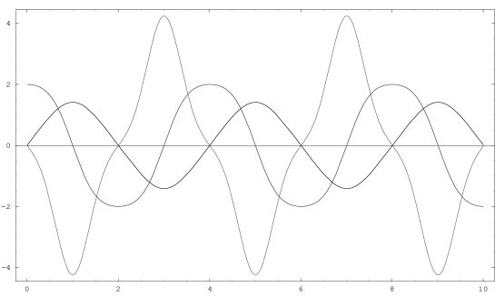
Figure 1: In decreasing gray level position, velocity and acceleration of a particle of unit mass in the quartic potential $V(q)=q^{2}/2+q^{4}/4$. The acceleration is minimal (maximal) and negative (positive) at odd (even) turning points of the velocity.

Let $x_{\mathit{c}\ell}(t;E)$ be the phase space lift of a trajectory on a periodic orbit of prime period $T_{cl}(E)$. A suitable basis for the linearised dynamics is represented by the Jacobi fields $\dot{x}(t;E)$, $\partial_{E}x(t;E)$. Linear independence is guaranteed by the invariance of the skew product

$$(\partial_{E}x_{\mathit{c}\ell}^{\dagger}\,\mathsf{J}\dot{x}_{\mathit{c}\ell})(t;E):=\,(\partial_{E}p_{\mathit{c}\ell}\,\dot{q}_{\mathit{c}\ell}-\,\partial_{E}q_{\mathit{c}\ell}\,\dot{p}_{\mathit{c}\ell})(t;E)=\left.\frac{d\mathcal{H}}{dE}\right|_{x_{\mathit{c}\ell}(t;E)}\!\!\!\!\!\!\!\!=1$$ (258)

The skew product coincides with the Wronskian determinant of the linearised dynamics. In fig. 2 the two Jacobi fields are plotted for (256). The Jacobi field of the second kind $\partial_{E}x(t;E)$ describes a linear instability [129, 51]

$$\partial_{E}x(t;E):=\kappa\,\frac{t-T^{\prime}}{T_{\mathit{c}\ell}}\,\dot{x}_{\mathit{c}\ell}(t;E)+\left.\left(\frac{\partial x}{\partial E}\right)(t;E)\right|_{\frac{t-T^{\prime}}{T_{cl}}=\mathrm{const.}}$$ (259)

with

$$\kappa:=-\,\frac{dT_{\mathit{c}\ell}}{dE}$$ (260)

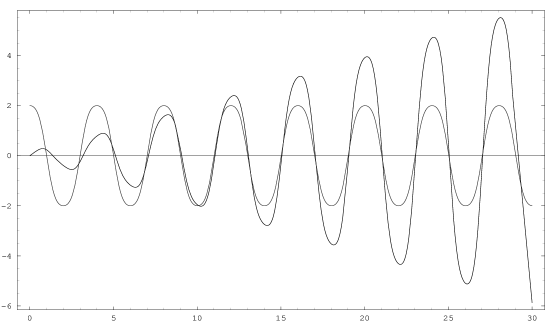
Figure 2: The Jacobi fields $\dot{q}_{\mathit{c}\ell}$ and $\partial_{E}q_{\mathit{c}\ell}$ relative to the motion of a particle of unit mass in the potential $V(q)=q^{2}/2+q^{4}/4$. The envelope of the amplitude peaks of the non periodic Jacobi field $\partial_{E}q_{\mathit{c}\ell}$ is linear with slope $-dT_{\mathit{c}\ell}/dE$. The conservation of the skew product imposes the non periodic Jacobi fields to be positive at odd turning points of the velocity.

The linearised flow in phase space is (compare with formula (610) in appendix E)

$$\mathsf{F}(t,T^{\prime})=[\dot{x}_{\mathit{c}\ell}(t;E),\partial_{E}x(t;E)]\,[\dot{x}_{\mathit{c}\ell}(T^{\prime};E),\partial_{E}x(T^{\prime};E)]^{-1}$$ (261)

The Sturm-Liouville operator associated to the second variation along a trajectory of energy $E$ is

$$L\,=\,-\,m\,\frac{d^{2}}{dt^{2}}-\left(\frac{d^{2}U}{dq^{2}}\right)(q_{\mathit{c}\ell}(t;E))$$ (262)

By (261) the Morse index for Dirichlet boundary conditions is determined by the number of zeroes of

$$\mathsf{B}(t,T^{\prime})=\partial_{E}q_{\mathit{c}\ell}(t;E)\,\dot{q}_{\mathit{c}\ell}(T^{\prime};E)-\partial_{E}q_{\mathit{c}\ell}(T^{\prime},E)\,\dot{q}_{\mathit{c}\ell}(t;E)$$ (263)

The right hand side is a linear combination of solutions of the linearised dynamics. Hence it is itself a Jacobi field vanishing at $t$ equal $T^{\prime}$. The zeroes encountered by (263) in $]T,T^{\prime}[$ define the number of conjugate points and therefore the Morse index associated to Dirichlet boundary conditions in the interval $[T^{\prime},T]$. By (263) also follows that if $q_{\mathit{c}\ell}$ starts from a turning point, ($\dot{q}_{\mathit{c}\ell}$ equal zero), the index will be specified by the number of turning points encountered in $]T^{\prime},T[$.

Let now $T$ be equal to $r\,T_{cl}$ with $r$ a positive integer. Furthermore suppose the trajectory $q_{\mathit{c}\ell}$ to start form a generic point (not a turning point) on the periodic orbit. Observe that $\mathsf{B}(t,T^{\prime})$ starts with positive derivative and has the same signature of $\kappa$ over multiples of the period. Moreover from the Wronskian condition (258) on a turning point

$$1=-\,(\partial_{E}q_{\mathit{c}\ell}\,\dot{p}_{\mathit{c}\ell})(t_{\mathrm{t.p,}};E)$$ (264)

follows that $\mathsf{B}(t,T^{\prime})$ must change sign at least once over one period, since velocity and acceleration change sign twice. Hence

$$\mathrm{ind}^{-}L_{\mathrm{Dir.}}([T^{\prime},T^{\prime}+rT_{\mathit{c}\ell}])\,=\,2\,r-\frac{1-\mathrm{sign}\kappa}{2}$$ (265)

If instead the trajectory starts from a turning point then

$$\mathrm{ind}^{-}L_{\mathrm{Dir.}}([T^{\prime},T^{\prime}+rT_{\mathit{c}\ell}])=2\,r-1$$ (266)

Associating periodic boundary conditions to the differential operation (262) in the same interval $[T^{\prime},T^{\prime}+r\,T_{\mathit{c}\ell}]$ defines the self-adjoint Sturm-Liouville operator $L_{\mathrm{Per.}}$. The periodic Morse index is determined from the sum of the Dirichlet index and the order of concavity. This latter is read from the monodromy matrix

$$\mathsf{M}=\left[\begin{array}[]{cc}1+\frac{dT_{\mathit{c}\ell}}{dE}(E)\,(\dot{p}_{\mathit{c}\ell}\dot{q}_{\mathit{c}\ell})(T_{cl};E)&\,\,-\frac{dT_{\mathit{c}\ell}}{dE}(E)\,\dot{q}_{\mathit{c}\ell}^{2}(T_{cl};E)\\ \frac{dT_{\mathit{c}\ell}}{dE}(E)\,\dot{p}_{\mathit{c}\ell}^{2}(T_{\mathit{c}\ell};E)&\,\,1-\frac{dT_{\mathit{c}\ell}}{dE}(E)\,(\dot{p}_{\mathit{c}\ell}\dot{q}_{\mathit{c}\ell})(T_{\mathit{c}\ell};E)\end{array}\right]$$ (269)

If the starting point of the periodic trajectory is taken in generic position, the order of concavity is specified by (254) and vanishes identically:

$$\mathrm{ind}^{-}L_{\mathrm{Per.}}([T^{\prime},T^{\prime}+rT_{\mathit{c}\ell}])=2\,r-\frac{1-\mathrm{sign}\kappa}{2}$$

$$\mathrm{nul}L_{\mathrm{Per.}}([T^{\prime},T^{\prime}+rT_{\mathit{c}\ell}])=1$$ (270)

Figure 3: The period $T_{\mathit{c}\ell}$ of a particle of unit mass in the potential $V(q)=q^{2}/2+q^{4}/4$ plotted versus the energy. The period decreases from the value $T_{\mathit{c}\ell}(0)=2\,\pi$, the period of the harmonic oscillator, with asymptotic behaviour $T_{\mathit{c}\ell}(E)\sim E^{-\,1/4}$ for $E$ tending to infinity.

If instead the trajectory starts from a turning point, the general index formula (244) must be applied. To the index (266) must be added a non zero contribution from the order of concavity. The non zero contribution comes from the recurrent Jacobi field

$$\jmath_{\mathrm{rec.}}(t)=\dot{q}_{\mathit{c}\ell}(t;E)\partial_{E}p_{\mathit{c}\ell}(T^{\prime};E)-\partial_{E}q_{\mathit{c}\ell}(t;E)\dot{p}_{\mathit{c}\ell}(T^{\prime};E)$$ (271)

with now

$$\dot{q}_{\mathit{c}\ell}(T^{\prime}+rT_{\mathit{c}\ell};E)=0$$ (272)

and it is equal to

$$\delta^{2}\mathcal{S}(\jmath_{\mathrm{rec.}},\jmath_{\mathrm{rec.}})=\mathsf{M}_{2\,1}=\frac{dT_{\mathit{c}\ell}}{dE}(E)\dot{p}_{\mathit{c}\ell}^{2}(T_{\mathit{c}\ell};E)$$ (273)

The sum of the Dirichlet index and of the order of concavity recovers (270). In the case of the Hamiltonian (256) the index is seen to be even since the period is a monotonically decreasing function of the energy (fig. 3).

ii Harmonic oscillator

The counting of the conjugate points in $[0,T]$ yields (231)

$$\mathrm{ind}^{-}L_{\mathrm{Dir.}}([0,T])=\#(\mbox{zeroes of}\sin(\omega t)\,\,\mbox{in}\,]0,T[)=\mathrm{int}\left[\frac{\omega T}{\pi}\right]$$ (274)

in agreement with the computations of section 3.1.1 and of appendix H.0.2. In consequence, the periodic Morse index is

$$\mathrm{ind}^{-}L_{\mathrm{Per.}}([0,T]) = \mathrm{ind}^{-}L_{\mathrm{Dir.}}([0,T])+\mathrm{ind}^{-}\frac{\cos(\omega\,T)-1}{\sin(\omega\,T)}$$ (275)

$$= 1+2\,\mathrm{int}\left[\frac{\omega T}{2\,\pi}\right]$$

for $T$ generic.

3.4 Crossing forms and Maslov indices

The constructions of Morse indices of the previous two sections are reconciled if a more general topological framework is developed to investigate the spectral flow. This was done by Duistermaat in [56] who refined ideas introduced by Bott in [29].

First, the following heuristic argument helps to understand the topological invariance of the Morse index. The Morse index of a self-adjoint $L_{\mathfrak{B}}$ is the number of negative eigenvalues

$$\mathrm{ind}^{-}L_{\mathfrak{B}}=\sum_{\ell_{j}\,\in\,\mathrm{Sp}L_{\mathfrak{B}}}\theta(-\ell_{j})$$ (276)

If $L_{\mathfrak{B}}$ is embedded into a smooth $n$-parameters family of self-adjoint Sturm-Liouville operators including a positive definite element, the index can be thought as the line integral in the space of the parameters connecting $L_{\mathfrak{B}}$ to the positive definite element. Parametrising with $\tau$ such curve, the index takes the form

$$\mathrm{ind}^{-}L_{\mathfrak{B}} = \,-\,\sum_{\ell_{n\,,\tau}\,\in\,\mathrm{Sp}L_{\mathfrak{B}\,,\tau}}\int_{0}^{\tau^{\prime}}d\tau\,\partial_{\tau}\,\theta(-\ell_{n\,,\tau})$$ (277)

$$= \sum_{\ell_{n\,,\tau}\,\in\,\mathrm{Sp}L_{\mathfrak{B}\,,\tau}}\int_{0}^{\tau^{\prime}}d\tau\,\frac{\partial\ell_{n\,,\tau}}{\partial\tau}\,\delta(\ell_{n\,,\tau})$$

where it is assumed that zero and $\tau^{\prime}$ correspond respectively to $L_{\mathfrak{B}}$ and the positive definite operator. In order the equality to hold true, only regular crossing of zero modes are supposed to occur. The topological invariance of the index stems from the identical vanishing of loop integrals over exact differentials which ensures the independence of the index of the curve used to compute (277).

The last equality in (277) states that along any curve in the space of self-adjoint Sturm-Liouville operators, the Morse index is specified by the sign of the eigenvalue flow on zero modes. Proceedings as in section 3.2.1 yields

$$\partial_{\tau}\ell_{n\,,\tau}=\langle\lambda_{n\,,\tau}\,,(\partial_{\tau}L_{\mathfrak{B}\,,\tau})\lambda_{n\,,\tau}\rangle$$ (278)

The integral localises on zero modes. Differentiating the Jacobi equation

$$(L_{\tau}\,\jmath_{\tau})(t)=0$$ (279)

versus the curve parameter $\tau$ allows to prove the chain of equalities

$$\langle\jmath_{\tau}\,,(\partial_{\tau}L_{\tau})\jmath_{\tau}\rangle\,=\,-\,\langle\jmath_{\tau}\,,L_{\tau}\partial_{\tau}\jmath_{\tau}\rangle\,=\,\beth(\jmath\,,\partial_{\tau}\jmath_{\tau})$$ (280)

The restriction to a crossing point defines the crossing form [56, 136, 137, 138]:

$$\daleth(\mathsf{F}_{\tau}(T,T^{\prime}),\mathfrak{B}):=\beth(\jmath_{\tau}\,,\partial_{\tau}\jmath_{\tau})|_{\mathfrak{B}\,\cap\,\mathrm{Gr}\mathsf{F}_{\tau}(T,T^{\prime})}$$ (281)

The requirement of smoothness of the deformation can be weakened. Provided the spectral flow is continuous, discontinuous non vanishing derivatives of the zero eigenvalues also allow to infer the direction of the spectral flow.
The Morse index of $L_{\mathfrak{B}}$ is

$$\mathrm{ind}^{-}L_{\mathfrak{B}}\,=\,\!\!\sum_{\{\,\tau\,>\,0|\mathfrak{B}\cap\mathrm{Gr}\mathsf{F}_{\tau}(T,T^{\prime})\,\}}\!\!\mathrm{sign}\daleth(\mathsf{F}_{\tau}(T,T^{\prime}),\mathfrak{B})$$ (282)

for any homotopy transformation with only regular crossings connecting $L_{\mathfrak{B}}$ to a positive definite Sturm-Liouville operator. The sign of the crossing form over a discontinuous derivative is the arithmetic average of the derivatives from the left and the right of the critical value of $\tau$.
The crossing forms (236) produced by deformations of the time interval are particular examples. The fact is recognised by looking at the explicit expression of crossing forms. A crossing occurs each time for some $x,y\,\in\,\mathbb{R}^{2d}$ the equality holds

$$\left[\begin{array}[]{c}\mathsf{Z}_{1}\,y\\ \mathsf{Z}_{2}\,y\end{array}\right]=\mathrm{Gr}\mathsf{F}_{\tau}x$$ (285)

$(\mathsf{Z}_{1}\,,\mathsf{Z}_{2})$ being the Bott pair describing $\mathfrak{B}$. Hence (281) is equivalent to

$$\daleth(\mathsf{F}_{\tau}(T,T^{\prime}),\mathfrak{B})\,=\,-\,\left.\mathsf{Z}_{1}^{\dagger}\,\left(\mathsf{F}_{\tau}^{\dagger}\,\mathsf{J}\,\frac{\partial\mathsf{F}_{\tau}}{\partial\tau}\right)(T,T^{\prime})\,\mathsf{Z}_{1}\,\,\right|_{\mathrm{Gr}\mathsf{F}_{\tau}(T,T^{\prime})\,\cap\,\mathfrak{B}}$$ (286)

The matrix on the right hand side is symmetric at glance since smooth deformation of symplectic matrices are governed by linear Hamiltonian equations (appendix E.2.3).

The formulae (285), (286) disclose the possibility to define the Morse index of a self-adjoint Sturm-Liouville operator as the index of homotopy transformations of finite dimensional quadratic forms. Namely an arbitrary deviation from the crossing condition (285) can be written in the form

$$\left[\begin{array}[]{c}\mathsf{Z}_{1}\,y\\ \mathsf{Z}_{2}\,y\end{array}\right]+\left[\begin{array}[]{c}\mathsf{V}_{1}\,z\\ \mathsf{V}_{2}\,z\end{array}\right]=\mathrm{Gr}\mathsf{F}_{\tau}(T,T^{\prime})x\,,\quad\quad x,y,z\,\in\,\mathbb{R}^{2d}$$ (291)

provided the Bott pair $(\mathsf{V}_{1}\,,\mathsf{V}_{2})$ spans in the sense of section 3.1, some linear complement $\mathfrak{V}$ in $\mathbb{R}^{4\,d}$ of $\mathrm{Gr}\mathsf{F}_{\tau}$ and $\mathfrak{B}$. In such a case (291) admits always solution for $z$

$$[\mathsf{Z}_{2}-\mathsf{F}_{\tau}\mathsf{Z}_{1}\,]y=[\mathsf{V}_{2}-\mathsf{F}_{\tau}\mathsf{V}_{1}\,]z$$ (292)

On solutions $\bar{z}_{\tau}$ the symplectic form on $\mathfrak{B}$

$$\beth|_{\mathfrak{B}}:=\left[\begin{array}[]{c}\mathsf{V}_{1}\,\bar{z}_{\tau}\\ \mathsf{V}_{2}\,\bar{z}_{\tau}\end{array}\right]^{\dagger}\left[\begin{array}[]{cc}\mathsf{J}&0\\ 0&-\mathsf{J}\end{array}\right]\left[\begin{array}[]{c}\mathsf{Z}_{1}\,y\\ \mathsf{Z}_{2}\,y\end{array}\right]$$ (299)

defines the family of symmetric matrices in $\mathbb{R}^{2d}\times\mathbb{R}^{2d}$:

$$\mathcal{Q} \!(\mathfrak{B},\mathfrak{V};\mathrm{Gr}\,\mathsf{F}_{\tau}):=$$ (300)

$$\frac{1}{2}\left\{[\mathsf{Z}_{2}^{\dagger}\mathsf{J}\mathsf{V}_{2}-\mathsf{Z}_{1}^{\dagger}\mathsf{J}\mathsf{V}_{1}][\mathsf{V}_{2}-\mathsf{F}_{\tau}\mathsf{V}_{1}\,]^{-1}[\mathsf{Z}_{2}-\mathsf{F}_{\tau}\mathsf{Z}_{1}\,]+c.c.\right\}$$

The spectrum of $\mathcal{Q}(\mathfrak{B},\mathfrak{V};\mathrm{Gr}\,\mathsf{F}_{\tau})$ contains a zero if and only if the parameter $\tau$ attains a value $\tau^{\star}$ such that $L_{\mathfrak{B}\,,\tau^{\star}}$ has a zero mode. Furthermore a direct computation shows that

$$\mathrm{sign}\mathcal{Q}(\mathfrak{B},\mathfrak{V};\mathrm{Gr}\,\mathsf{F}_{\tau^{\star}+d\tau})=\mathrm{sign}\mathcal{Q}(\mathfrak{B},\mathfrak{V};\mathrm{Gr}\,\mathsf{F}_{\tau^{\star}})+\mathrm{sign}\daleth(\mathsf{F}_{\tau^{\star}},\mathfrak{B})$$ (301)

Proceeding in this way, the Morse index of a self-adjoint Sturm-Liouville operator is identified with the Maslov index, the index of the graph of a continuous curves in $Sp(2\,d)$ having only regular crossings with a given Lagrangian subspace $\mathfrak{B}$ of $\mathbb{R}^{4d}$ [8, 90, 56, 136]. The identification permits to evaluate the Morse index without making direct reference to the corresponding operator. In contrast to the eigenvalues of the Sturm-Liouville operator, the eigenvalues of the finite dimensional quadratic form (300) as functions of $\tau$ can also change sign by diverging. The circumstance insures that arbitrary large values of the Morse index are eventually attained.

According to Robbin and Salamon [136], the Maslov index of the graph $\mathrm{Gr}\,\mathsf{S}_{\tau}$ of any one parameter family of matrices $\mathsf{S}(\tau)$ in $Sp(2d)$ is defined as

$$\aleph(\mathsf{S}(\tau), \mathfrak{B} ,[\tau_{1},\tau_{2}])=\frac{1}{2}\,\mathrm{sign}\daleth(\mathsf{S}(\tau_{1}),\mathfrak{B})$$ (302)

$$+ \!\!\sum_{\begin{subarray}{c}\tau_{1}<\tau<\tau_{2}\,\\ \tau|\mathrm{Gr}\mathsf{S}(\tau)\in\mathfrak{B}\end{subarray}}\!\!\!\!\!\mathrm{sign}\daleth(\mathsf{S}(\tau),\mathfrak{B})+\frac{1}{2}\,\mathrm{sign}\daleth(\mathrm{Gr}\mathsf{S}(\tau_{2}),\mathfrak{B})$$

End-points contribute of course only if an intersection occurs there. Maslov indices (302) enjoy the following properties.

1. Naturality: the index is invariant under a simultaneous symplectic transformation $\mathbf{\Psi}$ of $\mathfrak{B}$ and $\mathrm{Gr}\mathsf{S}(\tau)$:

   $$\aleph(\Psi\,\mathsf{S}(\tau)\,,\Psi\,\mathfrak{B}\,,[\tau_{1},\tau_{2}])=\aleph(\mathsf{S}(\tau)\,,\mathfrak{B}\,,[\tau_{1},\tau_{2}])$$ (303)

   for all $\mathbf{\Psi}=(\Psi_{1}\,,\Psi_{2})$ leaving invariant the symplectic form $\beth$ in $\mathbb{R}^{4d}$

   $$\Psi_{1}^{\dagger}\,\mathsf{J}\,\Psi_{1}=\Psi_{2}^{\dagger}\,\mathsf{J}\,\Psi_{2}$$ (304)

2. Catenation: for $\tau_{1}\,<\,\tau_{2}<\,\tau_{3}$

   $$\aleph(\mathsf{S}(\tau)\,,\mathfrak{B}\,,[\tau_{1},\tau_{3}])=\aleph(\mathsf{S}(\tau)\,,\mathfrak{B}\,,[\tau_{1},\tau_{2}])+\aleph(\mathsf{S}(\tau)\,,\mathfrak{B}\,,[\tau_{2},\tau_{3}])$$ (305)

3. Product: if the curve $\mathsf{S}(\tau)=\mathsf{S}^{(1)}(\tau)\oplus\mathsf{S}^{(2)}(\tau)$ and the Lagrangian subspace $\mathfrak{B}=\mathfrak{B}^{(1)}\oplus\mathfrak{B}^{(2)}$

   $$\aleph(\mathsf{S}^{(1)}(\tau) \!\!\oplus\mathsf{S}^{(2)}(\tau),\mathfrak{B}^{(1)}\oplus\mathfrak{B}^{(2)},[\tau_{1},\tau_{2}])=$$ (306)

   $$\aleph(\mathsf{S}^{(1)}(\tau),\mathfrak{B}^{(1)},[\tau_{1},\tau_{2}])+\aleph(\mathsf{S}^{(2)}(\tau),\mathfrak{B}^{(2)},[\tau_{2},\tau_{3}])$$

4. Homotopy: the Maslov index is invariant under fixed end-points homotopies.

Of the above properties the first three are immediate consequence of the definition. Homotopy was first proven by Arnol’d in [8]. The proof proceeds by showing that the signature of the crossing form defines a Brouwer degree [113, 68] for the crossing. The homotopy invariance of the Brouwer degree is then a standard result of differential topology [113].

One can use Maslov indices to compute the Morse index of a self-adjoint Sturm-Liouville operator $L_{\mathfrak{B}^{(a)}}$ with respect to the Morse index of a second one $L_{\mathfrak{B}^{(b)}}$. Under the hypothesis that both $\mathfrak{B}^{(a)}$ and $\mathfrak{B}^{(b)}$ have no intersections with $\mathrm{Gr}\,\mathsf{S}(\tau)$ at path end-points $\tau_{1}$, $\tau_{2}$, Hörmander proved in ref. [90] section $3.3$ the equality

$$\aleph(\mathsf{S}(\tau),\mathfrak{B}^{(a)}\,,[\tau_{1},\tau_{2}])=\aleph(\mathsf{S}(\tau),\mathfrak{B}^{(b)}\,,[\tau_{1},\tau_{2}])+$$

$$\frac{1}{2}\left[\mathrm{sign}\mathcal{Q}(\mathfrak{B}^{(b)},\mathrm{Gr}\mathsf{S}(\tau_{2});\mathfrak{B}^{(a)})-\mathrm{sign}\mathcal{Q}(\mathfrak{B}^{(b)},\mathrm{Gr}\mathsf{S}(\tau_{1});\mathfrak{B}^{(a)})\right]$$ (307)

Replacing $\mathsf{S}(\tau)$ with $\mathsf{F}(\tau,T^{\prime})$ shows that Hörmander’s relation is a generalisation of the relation (253) between the indices of Dirichlet and periodic boundary conditions.

Homotopy and Hörmander’s identity (307) provide all the needed tools to understand the origin of the different prescriptions given in the literature for the evaluation of Morse indices. The following sections are devoted to illustrate this point.
The reader interested in a more detailed presentation of Maslov index theory will enjoy the very accessible and comprehensive presentation by Robbin and Salamon in ref. [136]. The needed basic background in topology can be found in [113].

3.5 Topological construction of Morse indices

Using the results of the previous section, the Morse index of $L_{\mathfrak{B}}$, $\mathfrak{B}\sim(\mathsf{Z}_{1},\mathsf{Z}_{2})$ can be computed from any closed loop formed by varying $\mathsf{F}_{\tau}(t,T^{\prime})$ in the $(\tau,t)$-plane. It comprises the following oriented paths

Figure 4: The homotopy loop

1. $\qquad\mathsf{F}_{\tau}(T,T^{\prime})\,,\qquad\qquad d\tau\,\leq\,\tau\,\leq\,\tau^{\prime}$
   The flow $\mathsf{F}_{\tau}(T,T^{\prime})$ is solution of (196) with the family of Hamiltonian matrices generated by adding a positive definite potential term as in section 3.1. The initial value $d\tau$ provides for an arbitrary small positive deformation which removes eventual zero modes. The upper value $\tau^{\prime}$ is chosen large enough such that the Sturm-Liouville operator becomes positive definite. Thus, the Maslov index of the path coincides with Morse index of $L_{\mathfrak{B}}$:

   $$\aleph_{1}(\mathsf{F},\mathfrak{B})=\mathrm{ind}^{-}L_{\mathfrak{B}}([T^{\prime},T])=\sum_{\begin{subarray}{c}\tau>0\\ \mathfrak{B}\cap\mathrm{Gr}\mathsf{F}_{\tau}(T,T^{\prime})\end{subarray}}\!\!\!\!\!\!\mathrm{nul}\{\mathsf{Z}_{2}-\mathsf{F}_{\tau}(T,T^{\prime})\mathsf{Z}_{1}\}$$ (308)

2. $\qquad\mathsf{F}_{\tau^{\prime}}(t,T^{\prime})\,,\qquad\qquad T\,\geq\,t\,\geq\,T^{\prime}$
   For $\tau$ large enough the operator is dominated by the positive definite potential. No zero mode can occur until $t$ reaches $T^{\prime}$ since the quadratic form (189) is positive definite for all $t$ strictly larger than $T^{\prime}$. At initial time the condition

   $$\mathsf{F}_{\tau}(T^{\prime},T^{\prime})=\mathsf{I}_{2d}\,,\qquad\qquad\forall\,\tau$$ (309)

   may generate an intersection between $\mathfrak{B}$ and $\mathrm{Gr}\,\mathsf{I}_{2d}$. The Maslov index (302) is in such a case

   $$\aleph_{2}(\mathsf{F},\mathfrak{B})=\,\frac{1}{2}\,\mathrm{sign}\left\{\left.\mathsf{Z}_{2}^{\dagger}\,\mathsf{H}_{\tau^{\prime}}(T^{\prime})\mathsf{Z}_{2}\,\,\right|_{\mathrm{Gr}\,\mathsf{I}_{2d}\,\cap\,\mathfrak{B}}\right\}$$ (310)

   since the crossing form can be directly expressed in terms of the Hamiltonian matrix (199). The sign is the opposite than in (281) due to the negative orientation of the path.

3. $\qquad\mathsf{F}(t,T^{\prime})\,,\qquad\qquad T^{\prime}\,\leq\,t\,\leq\,T$
   The corresponding Maslov index is

   $$\aleph_{3} \!\!(\mathsf{F},\mathfrak{B})=\,-\,\frac{1}{2}\,\mathrm{sign}\left\{\left.\mathsf{Z}_{2}^{\dagger}\,\mathsf{H}(T^{\prime})\mathsf{Z}_{2}\,\right|_{\mathrm{Gr}\,\mathsf{I}_{2d}\,\cap\,\mathfrak{B}}\,\right\}$$ (311)

   $$-\!\!\!\!\!\!\sum_{\begin{subarray}{c}T^{\prime}<t<T\,\\ t|\mathrm{Gr}\,\mathsf{F}(t,T^{\prime})\cap\mathfrak{B}\end{subarray}}\!\!\!\!\!\!\!\!\mathrm{sign}\{\mathsf{Z}_{2}^{\dagger}\,\mathsf{H}(t)\mathsf{Z}_{2}\,\}-\frac{1}{2}\,\mathrm{sign}\left\{\left.\mathsf{Z}_{2}^{\dagger}\,\mathsf{H}(T)\mathsf{Z}_{2}\,\right|_{\mathrm{Gr}\mathsf{F}(T,T^{\prime})\cap\mathfrak{B}}\right\}$$

4. $\qquad\mathsf{F}_{\tau}(T,T^{\prime})\,,\qquad\qquad 0\,\leq\,\tau\,\leq\,d\tau$
   By construction the last branch may encounter a Lagrangian intersection only in the initial point. The Maslov index is therefore

   $$\aleph_{4}(\mathsf{F},\mathfrak{B}) = -\,\frac{1}{2}\,\mathrm{sign}\left\{\left.\mathsf{Z}_{1}^{\dagger}\,\left(\mathsf{F}_{\tau}^{\dagger}\,\mathsf{J}\,\frac{\partial\mathsf{F}_{\tau}}{\partial\tau}\right)(T,T^{\prime})\,\mathsf{Z}_{1}\,\,\right|_{\tau=0\,,\mathrm{Gr}\mathsf{F}(T,T^{\prime})\,\cap\,\mathfrak{B}}\right\}$$ (312)

   $$=\frac{1}{2}\,\mathrm{nul}\{\mathsf{Z}_{2}-\mathsf{F}(T,T^{\prime})\mathsf{Z}_{1}\,\}$$

   The last equality holds true because increasing $\tau$ begets by construction only positive definite crossing forms along this branch of the homotopy path.

The Maslov index of the overall loop is zero

$$\sum_{i=1}^{4}\aleph_{i}(\mathsf{F},\mathfrak{B})=0$$ (313)

Therefore it follows

$$\mathrm{ind}^{-}L_{\mathfrak{B}}([T^{\prime},T])=\aleph_{1}(\mathsf{F},\mathfrak{B})\,=\,-[\aleph_{2}(\mathsf{F},\mathfrak{B})+\aleph_{3}(\mathsf{F},\mathfrak{B})+\aleph_{4}(\mathsf{F},\mathfrak{B})]$$ (314)

The Maslov index of the second branch of the loop can be evaluated a priori. For any $\tau$ the Hamiltonian matrix (199) is similar to

$$(\mathsf{O}\,\mathsf{H}\,\mathsf{O}^{-1})_{\tau}(t)=\left[\begin{array}[]{cc}-\mathsf{L}_{q\,q}-\tau\,\mathsf{U}&\quad 0\\ 0&\quad\mathsf{L}_{\dot{q}\,\dot{q}}^{-1}\end{array}\right]\!(t)$$ (317)

for $\mathsf{O}$ a suitable non singular matrix. For $\tau$ large enough, (317) is the orthogonal sum of two $d\,\times\,d$ dimensional blocks with opposite sign definition. The observation recovers the result (241) obtained for local boundary conditions. If $\mathsf{Z}_{2}=0\oplus\mathsf{I}_{d}$ the Morse index coincides with the number of crossings counted with their degeneration in the open time interval $]T^{\prime},T[$. Any overlap of the Bott matrix $\mathsf{Z}_{2}$ with the position space produces a non trivial generalisation of the order of concavity defined in subsection 3.2.2 for the particular case of periodic boundary conditions. Homotopy invariance of Maslov indices and Hörmander’s identity (307) endow with great freedom in the choice of the representation of the Morse index which most suits the analysis of the physical origin of the contributions. Periodic boundary conditions well illustrate the general situation.

3.6 Morse index and structural stability of periodic orbits

The difference $T-T^{\prime}$ is in this section supposed to be equal or a multiple of the period of the Sturm-Liouville operator.
The Bott pair describing periodic boundary conditions is $(\mathsf{Z}_{1}\,,\mathsf{Z}_{2})=(\mathsf{I}_{2d},\mathsf{I}_{2d})$. Therefore the Maslov index of the second branch of the homotopy loop is zero.
Hörmander’s identity can be applied directly to the catenation of the second and fourth branch. The identification of $\mathfrak{B}^{(a)}$ with $(\mathsf{I}_{2d},\mathsf{I}_{2d})$ and of $\mathfrak{B}^{(b)}$ with any $\mathfrak{A}\sim(\mathsf{Z}_{1},\mathsf{Z}_{2})$ such that

$$\left\{\begin{array}[]{c}\mathfrak{A}\cap(\mathsf{I}_{2d},\mathsf{I}_{2d})=\emptyset\\ \mathfrak{A}\cap\mathrm{Gr}\mathsf{F}(T,T^{\prime})=\emptyset\end{array}\right.\quad\Leftrightarrow\quad\left\{\begin{array}[]{c}\det(\mathsf{Z}_{2}-\mathsf{Z}_{1})\,\neq\,0\\ \det[\mathsf{Z}_{2}-\mathsf{F}(T,T^{\prime})\mathsf{Z}_{1}]\,\neq\,0\end{array}\right.$$ (322)

yields

$$\sum_{i=2}^{4}\aleph_{i}\{\mathsf{F},(\mathsf{I}_{2d},\mathsf{I}_{2d})\}\!=\aleph_{3}(\mathsf{F},\mathfrak{A})+\frac{1}{2}\,\mathrm{sign}\mathcal{Q}(\mathfrak{A},\mathrm{Gr}\mathsf{F}(T,T^{\prime});(\mathsf{I}_{2d},\mathsf{I}_{2d})\,)$$ (323)

A more detailed proof can be found in theorem $4.3$ of ref. [56]. The signature and the index of any symmetric form $\mathcal{F}$ in $2d$ dimensions are connected by the relation

$$\mathrm{ind}^{-}\mathcal{F}=\frac{1}{2}\,[2d-\mathrm{Ker}\mathcal{F}-\mathrm{sign}\mathcal{F}]$$ (324)

Thus one can recast the periodic index in the form

$$\mathrm{ind}^{-}L_{\mathrm{Per.}}([T,T^{\prime}])=-\aleph_{3}(\mathsf{F},\mathfrak{A})+\mathrm{ind}^{-}\mathcal{Q}(\mathrm{Gr}\mathsf{F}(T,T^{\prime}),\mathfrak{A};(\mathsf{I}_{2d},\mathsf{I}_{2d})\,)-d$$ (325)

which is the final expression given by Duistermaat in ref. [56].

The topological expression of the periodic Morse index can be used to analyse how the stability properties of the linear flow $\mathsf{F}(t,T^{\prime})$ are reflected in the index. The use of homotopy simplifies the analysis. The idea is to embed the linear flow $\mathsf{F}(t,T^{\prime})$ into a family of curves in $Sp(2d)$ with fixed end points. By property $iv$ of section 3.4 the Maslov index is the same for any element of family. The Floquet representation of the linear flow

$$\mathsf{F}(t,0) = \mathsf{Pe}(t)\,\exp\left\{\frac{t}{T}\,\mathsf{J}^{\,\dagger}\!\!\int_{0}^{T}dt^{\prime}\,\mathsf{H}(t^{\prime})\right\}=:\mathsf{Pe}(t)\,e^{t\,\mathsf{J}^{\dagger}\,\bar{\mathsf{H}}}$$ (326)

is suited for the construction. In order to streamline the notation $T^{\prime}$ has been set to zero. The matrix $\mathsf{Pe}(t)$ is supposed to have prime period $T$, while $\bar{\mathsf{H}}$ is the average of the Hamiltonian over a period. The Floquet form is the element of the continuous family

$$\mathsf{G}(t,s)=\left\{\begin{array}[]{cc}\mathsf{Pe}[(1+s)\,t]\,e^{(1-s)\,t\,\mathsf{J}^{\dagger}\bar{\mathsf{H}}}&\quad 0\leq t\leq\frac{T}{2}\\ \mathsf{Pe}(t)\mathsf{Pe}^{-1}[s\,(t-T)]\,e^{[s\,(t-T)+t]\mathsf{J}^{\dagger}\bar{\mathsf{H}}}&\quad\frac{T}{2}\leq t\leq T\end{array}\right.$$ (329)

attained by setting $s$ equal to zero. The end points of the homotopy family are independent of $s$. In order the Floquet representation to be fully specified, it is necessary to fix a convention on the phase of the eigenvalues of the monodromy matrix:

$$\mathsf{M}:=e^{T\mathsf{J}^{\dagger}\bar{\mathsf{H}}}$$ (330)

A convenient choice is to restrict the phase to the interval $[0,2\,\pi[$. The choice attributes to the exponential matrix in the Floquet representation a winding number equal to zero. Gel’fand and Lidskii introduced in [71] the winding number of a linear Hamiltonian flow as a topological characterisation of structural stability. In particular they proved that linear flows with the same monodromy and winding can be deformed into each other.

The tools forged above will now be used to compute the periodic Morse index in two different ways. The first is meant to illustrate the relation of the index with the stability properties of the flow, the second to recover the result of section 3.2.2.

3.6.1 The Conley and Zehnder index

The most direct way to evaluate the periodic index is to consider intersections of the homotopy loop with the periodic pair $(\mathsf{I}_{2d}\,,\mathsf{I}_{2d})$. The restriction to regular crossings imposes some conditions on the linear flows. In particular flows with parabolic normal forms must be regularised by a positive definite perturbation in order to render non singular the crossing form.
With this proviso, the index is equal to the Maslov index of the third branch of the homotopy loop (314). This latter is most conveniently computed at $s$ equal one for the family of symplectic curves (329):

$$\aleph_{3}\{\mathsf{F},(\mathsf{I}_{2d},\mathsf{I}_{2d})\} = \aleph\{\mathsf{Pe}(2\,t),(\mathsf{I}_{2d},\mathsf{I}_{2d}),[0,T/2]\}$$ (331)

$$+ \aleph\{e^{(2\,t-T)\,\mathsf{J}^{\dagger}\,\bar{\mathsf{H}}},(\mathsf{I}_{2d},\mathsf{I}_{2d}),[T/2,T]\}$$

The first Maslov index is independent of the Lagrangian manifold associated to the periodic Bott pair $(\mathsf{I}_{2d}\,,\mathsf{I}_{2d})$. The statement is proven by the following reasoning. Since the matrix $\mathsf{Pe}(t)$ is periodic its index does not change if the interval $[0,T/2]$ is replaced by $[t^{\prime},T/2+t^{\prime}]$ for any $t^{\prime}$ such that no intersection occurs. Hörmander’s identity (307) and periodicity then show

$$\aleph\{\mathsf{Pe}(2\,t),(\mathsf{I}_{2d},\mathsf{I}_{2d}),[0,T/2]\}=\aleph\{\mathsf{Pe}(2\,t),\mathfrak{A},[t^{\prime},T/2+t^{\prime}]\}$$ (332)

for any $\mathfrak{A}$ having no intersections with the graph of the flow at path end-points. In particular one can chose $\mathfrak{A}\sim(\mathsf{I}_{2d}\,,-\,\mathsf{I}_{2d})$ and observe that any symplectic matrix admits a unique polar representation

$$\mathsf{Pe}(2\,t)=(\mathsf{Sy}\,\mathsf{Or})(2\,t)\,,\qquad\left\{\begin{array}[]{l}\mathsf{Sy}(2\,t):=(\mathsf{Pe}^{\dagger}\mathsf{Pe})^{\frac{1}{2}}(2\,t)\\ \mathsf{Or}(2\,t):=[(\mathsf{Pe}^{\dagger}\mathsf{Pe})^{-\,\frac{1}{2}}\mathsf{Pe}](2\,t)\end{array}\right.$$ (335)

with both $\mathsf{Or}$ and $\mathsf{Sy}$ in $Sp(2d)$. The polar representation can be embedded into a family of curves analogous to (329). Since $\mathsf{Sy}$ is positive definite, crossing occurs only when

$$\det[\mathsf{I}_{2\,d}+\mathsf{Or}(2\,t)]=0$$ (336)

as $t$ ranges in $[0\,,T/2]$. The Maslov index can be thus computed from the intersection of the orthogonal matrix $\mathsf{Or}(2\,t)$ with the anti-periodic Bott pair.
An orthogonal and symplectic matrix admits in general the block representation

$$\mathsf{Or}=\left[\begin{array}[]{cc}\mathsf{X}&\quad\mathsf{Y}\\ -\mathsf{Y}&\quad\mathsf{X}\end{array}\right]\,,\qquad\qquad(\mathsf{X}+i\mathsf{Y})^{\dagger}(\mathsf{X}+i\mathsf{Y})=\mathsf{I}_{d}$$ (339)

and therefore it is similar to

$$\frac{1}{\sqrt{2}}\left[\begin{array}[]{lr}\mathsf{I}_{d}&\,\,-\,i\mathsf{I}_{d}\\ \mathsf{I}_{d}&\,\,i\,\mathsf{I}_{d}\end{array}\right]\left[\begin{array}[]{cr}\mathsf{X}&\,\,\mathsf{Y}\\ -\mathsf{Y}&\,\,\mathsf{X}\end{array}\right]\frac{1}{\sqrt{2}}\left[\begin{array}[]{lr}\mathsf{I}_{d}&\,\,i\mathsf{I}_{d}\\ \mathsf{I}_{d}&\,\,-i\,\mathsf{I}_{d}\end{array}\right]=\left[\begin{array}[]{lr}\mathsf{X}+i\,\mathsf{Y}&\,\,0\\ 0&\,\,\mathsf{X}-i\,\mathsf{Y}\end{array}\right]$$ (348)

The analysis of the crossing forms yields modulo four the equality

$$\aleph\{\mathsf{Pe}(2\,t) (\mathsf{I}_{2d},\mathsf{I}_{2d}),[0,T/2]\}=$$ , (349)

$$\frac{\mathrm{arg}\det[\mathsf{X}(T)+i\,\mathsf{Y}(T)]-\mathrm{arg}\det[\mathsf{X}(0)+i\,\mathsf{Y}(0)]}{\pi}\,,\quad\mathrm{mod}\,4$$

The right hand side is an integer by periodicity. It coincides with twice the Gel’fand and Lidskii [71] winding number of the linear periodic Hamiltonian flow $\mathsf{Pe}(2\,t)$.

The only contribution to the second Maslov index in (331) comes when $t$ is equal $T/2$. The crossing form can be straightforwardly evaluated from the normal forms of the stability blocks of the exponential flow. Following the same conventions of appendix 3.3 the Hamiltonian matrices associated to the blocks are

$$\bar{\mathsf{H}}|_{\mathrm{ell.}}=\left[\begin{array}[]{lr}\omega&\quad 0\\ 0&\omega\end{array}\right]\,,\qquad\bar{\mathsf{H}}|_{\mathrm{hyp}}=\left[\begin{array}[]{lr}0&\quad\omega\\ \omega&0\end{array}\right]$$ (354)

$$\bar{\mathsf{H}}|_{\mathrm{lox.}}=\left[\begin{array}[]{lr}0&\quad\omega\,(\mathsf{I}_{2}+\mathsf{J}_{2})\\ \omega\,(\mathsf{I}_{2}+\mathsf{J}_{2})^{\dagger}&0\end{array}\right]$$ (357)

A consequence of the analysis at the end of section E.2.2 is that inverse hyperbolic blocks behave at the origin as elliptic ones [59, 100]. The simplest parabolic blocks have the normal form

$$\left.\mathsf{F}(t,T^{\prime})\right|_{\mathrm{par.}}\,=\,\left[\begin{array}[]{cc}1&\quad\kappa\,\frac{t}{T}\\ 0&\quad 1\end{array}\right]$$ (360)

In appendix (E.2.3) it is shown that (360) bifurcates under a generic positive definite perturbation to an elliptic or to an hyperbolic block if, within the conventions adopted in this work, the sign of $\kappa$ is respectively negative or positive. In order to infer the sign of the infinitesimal characteristic frequencies of the elliptic blocks generated by the regularisation, one can reason as follows. A sufficiently small positive definite perturbation of the $L_{\mathrm{Per.}}([0,T])$ does not affect the periodic Morse index because it removes the zero modes while preventing any eigenvalue from turning negative. Therefore the value of the Maslov index associated to parabolic blocks by such a perturbation of the $L_{\mathrm{Per.}}([0,T])$ must coincide with the minimum over the set of the Maslov indices generated by arbitrary perturbations of the same system [107, 3, 4, 108]. This means that, once the Gel’fand-Lidskii winding number has been determined from the unperturbed system, the sign of the characteristic frequencies of elliptic blocks created by a positive definite perturbation must give rise to crossing forms with negative signature. A positive signature would produce a larger value of the Maslov index. A rigorous proof of the above perturbative argument can be found in [107].
Gathering the contributions of all blocks the resulting Maslov index is

$$\aleph\{e^{(2\,t-T)\,\mathsf{J}^{\dagger}\,\bar{\mathsf{H}}},(\mathsf{I}_{2d},\mathsf{I}_{2d}),[T/2,T]\}=n_{\mathrm{ell}}+n_{\mathrm{i.h.}}-\sum_{i=1}^{n_{\mathrm{p}}}\frac{1-\mathrm{sign}\,\kappa_{i}}{2}$$ (361)

where $n_{\mathrm{ell}}$, $n_{\mathrm{i.h.}}$ and $n_{\mathrm{p}}$ are respectively the number of elliptic and parabolic blocks in the monodromy matrix $\mathsf{M}=\mathsf{F}(T,0)$.

The overall periodic Morse index is

$$\mathrm{ind}^{-}L_{\mathrm{Per.}}([0,T])=n_{\mathrm{ell}}+n_{\mathrm{i.h.}}-\sum_{i=1}^{n_{\mathrm{p}}}\frac{1-\mathrm{sign}\,\kappa_{i}}{2}+2\,\mathfrak{w}$$ (362)

with $\mathfrak{w}$ the Gel’fand-Lidskii winding number. Elliptic and inverse hyperbolic blocks can therefore be associated with the occurrence of an odd number of negative eigenvalues in the spectrum of a periodic Sturm-Liouville operator $L_{\mathrm{Per.}}$.

In the mathematical literature [136, 137, 142, 110] the periodic Morse index expressed in the form (362) is often referred to as the Conley and Zehnder index. Conley and Zehnder [35] showed that the periodic Morse index (362) describes the foliation of the symplectic group $Sp(2d)$ in leaves of different winding. Each leaf further decomposes in two connected components characterised by opposite sign of the determinant

$$\mathrm{sign}\,\mathrm{det}[\mathsf{I}_{2d}-\mathsf{M}]=(-1)^{d-n_{\mathrm{ell}}-n_{\mathrm{i.h.}}}$$ (363)

In their paper [35], Conley and Zehnder analysed the stability properties of periodic orbits of non-autonomous Hamiltonian systems without parabolic blocks and in dimension larger than two. General proofs of the equivalence of the periodic Morse index with the Conley and Zehnder index were later given in [157, 3, 4] where the case of conservative systems with parabolic blocks is also encompassed.

It is straightforward to infer the behaviour of the index under iteration of a prime periodic orbit.
The winding number increases linearly with the number of repetitions $r$ of the orbit. The sign (363) may instead change according to a nonlinear law. Namely under iteration elliptic blocks of frequency $\omega$ experience further intersections if $r\,\omega$ becomes a multiple of $2\,\pi$. Inverse hyperbolic blocks generate a crossing form at each iteration since they are turned by even powers of the monodromy matrix into direct hyperbolic ones. Parabolic blocks do not change signature. Hence one concludes

$$\mathrm{ind}^{-} L_{\mathrm{Per.}}([0,r\,T])=$$ (364)

$$\sum_{i=1}^{n_{\mathrm{ell}}}\left[1+2\,\mathrm{int}\left(\frac{r\,\omega_{i}}{2\,\pi}\right)\right]+r\,n_{\mathrm{i.h.}}-\sum_{i=1}^{n_{\mathrm{p}}}\frac{1-\mathrm{sign}\,\kappa_{i}}{2}+2\,r\,\mathfrak{w}$$

The result holds for Hamiltonian systems without marginal degenerations. In [150], Sugita derived formulae (362), (364) by computing quadratic phase space trace path integrals on a time lattice. Sugita also pointed out that the negative sign in front of the parabolic block contribution renders in general the phase of the Gutzwiller trace formula independent from the signature of the energy block. A careful analysis of the behavior of the phase of the Gutzwiller trace formula predicted by (364) has been carried out in a recent paper by Pletyukhov and Brack [128] where several analytical and numerical examples are also investigated.
More general explicit expressions of the periodic Morse index in the Conley and Zehnder form, encompassing marginal degenerations can be found in the paper [108].

The behaviour of Morse indices of Sturm-Liouville operators of variational origin was investigated in the topological setting in ref. [40]. The same results can also be obtained by means of pure algebraic methods [94, 59].

Finally it is worth noting that the periodic Morse index can be identified with the winding number of the linear flow by applying the polar decomposition directly to $\mathsf{F}(t,0)$ [105, 140].

3.6.2 Focal point description

The periodic Morse index is needed in the Gutzwiller trace formula. Due to energy conservation at least one parabolic block is to be expected. Therefore in applications [140] it is useful to exploit Hörmander’s identity (307) to derive the index without need of perturbative arguments. Inserting $\mathfrak{A}\sim(\mathsf{I}_{d}\oplus 0\,,0\oplus\mathsf{I}_{d})$ in Duistermaat’s formula (325) yields:

$$\mathrm{ind}^{-}L_{\mathrm{Per.}}([0,T]) = \sum_{0\leq t\,<T}\mathrm{nul}\mathsf{D}(t,0)$$ (365)

$$+ \mathrm{ind}^{-}\mathcal{Q}(\mathrm{Gr}\mathsf{F}(T,0),\mathsf{I}_{d}\oplus 0\,,0\oplus\mathsf{I}_{d};(\mathsf{I}_{2d},\mathsf{I}_{2d})\,)-d$$

The matrix $\mathsf{D}$ is specified by the block representation of the flow (230). Some tedious algebra gives the expression of the concavity form:

$$\mathcal{Q}(\mathrm{Gr}\mathsf{F}(T,0) \!(\mathsf{I}_{d}\oplus 0\,,0\oplus\mathsf{I}_{d});(\mathsf{I}_{2d},\mathsf{I}_{2d})\,)$$ , (368)

$$= \left[\begin{array}[]{cc}(\mathsf{C}\mathsf{A}^{-1})(T,0)&\,\,\mathsf{A}^{\dagger\,-1}(T,0)-\mathsf{I}_{d}\\ \mathsf{A}^{-1}(T,0)-\mathsf{I}_{d}&\,\,-\,(\mathsf{A}^{-1}\mathsf{B})(T,0)\end{array}\right]$$

It is straightforward to see that in any vector basis where $\mathsf{B}(T,0)$ and $\mathsf{C}(T,0)$ vanish the index of (368) is equal to $d$. Thus the periodic index coincides with the zeroes encountered in the same vector basis by $\mathsf{D}(t,0)$ through all the time interval $[0,T]$.
More generally if $\mathsf{B}(T,0)$ is nonsingular then one finds

$$\mathrm{ind}^{-}\mathcal{Q}(\mathrm{Gr}\,\mathsf{F}(T,0),(\mathsf{I}_{d}\oplus 0\,,0\oplus\mathsf{I}_{d});(\mathsf{I}_{2d},\mathsf{I}_{2d})\,)=$$

$$\,\,\,\,\mathrm{ind}^{-}(\mathsf{D}\,\mathsf{B}^{-1}+\mathsf{B}^{-1}\mathsf{A}-\mathsf{B}^{-1}-\mathsf{B}^{-1\,\dagger})(T,0)+\mathrm{ind}^{-}[-(\mathsf{A}^{-1}\mathsf{B})(T,0)]$$ (369)

Under the same hypothesis the use of Hörmander’s identity gives

$$\sum_{0\leq t\,<T} \!\!\mathrm{nul}\mathsf{D}(t,0)=$$ (370)

$$\aleph_{3}\{\mathsf{F},(0\oplus\mathsf{I}_{d}\,,0\oplus\mathsf{I}_{d})\}+d-\mathrm{ind}^{-}[-(\mathsf{A}^{-1}\mathsf{B})(T,0)]$$

Since

$$\aleph_{3}\{\mathsf{F},(0\oplus\mathsf{I}_{d}\,,0\oplus\mathsf{I}_{d})\}=\sum_{0\,<t\,<T}\!\!\!\mathrm{nul}\mathsf{B}(t,0)$$ (371)

the expression of the periodic index given in section 3.2.2 is finally recovered.

The focal point representation can also be applied in a coordinate independent way. In particular it is possible to derive equation (362) (the Conley and Zehnder index), without need of the perturbative argument.
Consider for example a periodic Sturm-Liouville operator $L_{\mathrm{Per.}}([0,T])$ such that the associated linear flow consists of a parabolic and an elliptic block. The Floquet representation is then

$$\mathsf{F}(t,0)=\mathsf{Pe}(t)\,e^{t\,\mathsf{J}^{\dagger}\,\bar{\mathsf{H}}}=\mathsf{Pe}_{\mathrm{par.}}(t)\,e^{t\,\mathsf{J}^{\dagger}\,\bar{\mathsf{H}}_{\mathrm{par.}}}\oplus\mathsf{Pe}_{\mathrm{ell.}}(t)\,e^{t\,\mathsf{J}^{\dagger}\,\bar{\mathsf{H}}_{\mathrm{ell.}}}$$ (372)

As assumed above, phase $\omega t$ of the exponential matrix of the elliptic block is supposed to range in $[0,2\,\pi[$.

The product and homotopy properties of Maslov indices illustrated in section 3.4 permit to compute the periodic Morse index of $L_{\mathrm{Per.}}([0,T])$ as the sum of the Maslov indices of the stability blocks. Moreover, Hörmander equality (307) can be separately applied to the periodic and exponential matrices entering the Floquet representation. The Maslov index of the periodic matrix is already known to coincide with twice the Gel’fand and Lidskii winding number $\mathfrak{w}$.
In order to compute the Maslov index of $e^{t\,\mathsf{J}^{\dagger}\,\bar{\mathsf{H}}_{\mathrm{par.}}}$, $e^{t\,\mathsf{J}^{\dagger}\,\bar{\mathsf{H}}_{\mathrm{ell.}}}$ in $[0,T]$ one can apply Duistermaat formula (325) with $\mathfrak{A}\sim(1\oplus 0,0\oplus 1)$. Consider first the elliptic block:

$$e^{t\,\mathsf{J}^{\dagger}\,\bar{\mathsf{H}}_{\mathrm{ell.}}}=\left[\begin{array}[]{cc}\cos(\omega t)&\quad\sin(\omega t)\\ -\,\sin(\omega t)&\quad\cos(\omega t)\end{array}\right]$$ (375)

Crossings occur when

$$\det[(0\oplus 1)-e^{t\,\mathsf{J}^{\dagger}\,\bar{\mathsf{H}}_{\mathrm{ell.}}}(1\oplus 0)]=-\cos(\omega t)=0$$ (376)

The condition is satisfied if $\omega t$ is equal to $\pi/2$ or to $3\,\pi/2$. The corresponding crossing forms are equal to one. By equation (368) the order of concavity is

$$\mathrm{ind}^{-}\mathcal{Q}(\mathrm{Gr}e^{T\,\mathsf{J}^{\dagger}\,\bar{\mathsf{H}}_{\mathrm{ell.}}},(1\oplus 0\,,0\oplus 1);(\mathsf{I}_{2},\mathsf{I}_{2})\,)-1=$$

$$\quad\quad\mathrm{ind}^{-}\left[\begin{array}[]{cc}-\frac{\sin(\omega T)}{\cos(\omega T)}&\quad\frac{1}{\cos(\omega T)}-1\\ \frac{1}{\cos(\omega T)}-1&\quad-\frac{\sin(\omega T)}{\cos(\omega T)}\end{array}\right]-1$$ (379)

It is equal to one for $\omega T$ taking values in $[0\,,\pi/2]$, is zero for $\omega T$ in $]\pi/2\,,3\pi/2]$ and finally minus one for $\omega T$ in $]3\,\pi/2\,,2\,\pi]$. Adding up the contributions of the crossing and of the concavity forms one has:

$$\aleph\{e^{t\,\mathsf{J}^{\dagger}\,\bar{\mathsf{H}}_{\mathrm{ell.}}},(1\oplus 0\,,0\oplus 1),[0,T]\}=1$$ (380)

independently of the value $\omega T$ in $[0,2\,\pi[$.
Turning to the parabolic block eq. (360) , it is seen that the only non zero contribution comes from the order of concavity:

$$\mathrm{ind}^{-}\mathcal{Q}(\mathrm{Gr}e^{T\,\mathsf{J}^{\dagger}\,\bar{\mathsf{H}}_{\mathrm{par.}}},(1\oplus 0\,,0\oplus 1);(\mathsf{I}_{2},\mathsf{I}_{2})\,)-1=$$

$$\quad\quad\mathrm{ind}^{-}\left[\begin{array}[]{cc}0&\quad 0\\ 0&\quad-\kappa\end{array}\right]-1=-\frac{1-\mathrm{sign}\kappa}{2}$$ (383)

Gathering all terms one gets into

$$\mathrm{ind}^{-}L_{\mathrm{Per.}}([0,T[)=1-\frac{1-\mathrm{sign}\kappa}{2}+2\mathfrak{w}$$ (384)

which is formula (362) applied to the example considered here. The block by block analysis of the Maslov index, has been used by An and Long [4] to prove the equivalence of the Duistermaat formula (325) with the Conley and Zehnder index.

3.7 Phase space path integrals and infinite dimensional Morse theory

Classical mechanics has its natural formulation in phase space. The lift of configuration space quantities to phase space was reiteratively used in the above presentation of Morse index theory. It is therefore natural to wonder whether the treatment of the semiclassical approximation can be simplified by starting from phase space path integrals.

Formally, phase space path integrals can be written directly in the continuum by replacing the quadratic kinetic energy term in the configuration space Lagrangian with its Fourier transform [51, 101, 135, 165]. The propagator is then represented in the form

$$K(Q,T|Q^{\prime},T^{\prime})=\int_{q(T^{\prime})=Q^{\prime}}^{q(T)=Q}\mathcal{D}[q(t)p(t)]e^{i\int_{T^{\prime}}^{T}dt[p_{\alpha}\dot{q}^{\alpha}-\mathcal{H}(p,q)]}$$ (385)

The domain of integration is asymmetric between position and momentum variables as the boundary conditions impose a constraint only on position variables. More general phase space path integral expression are obtained if (385) is used to compute the time evolution of quantum observables other than the propagator.
Formally the derivation of the semiclassical approximation of section 2.2 goes through also for phase space path integrals. In the presence of boundary conditions $\mathfrak{B}$ of the form (66) it leads to the quadratic action

$$\delta^{2}\mathcal{S}=\int_{T^{\prime}}^{T}dt\,\delta x^{\alpha}\mathfrak{J}_{\alpha\,\beta}\delta x^{\beta}\,,\qquad\qquad\alpha\,,\beta=1,...,2\,d$$ (386)

where $\delta x=(\delta q,\delta p)$ denotes the fluctuations around the phase space classical trajectory $x_{\mathit{c}\ell}$ while

$$\mathfrak{J}_{\alpha\,\beta}:=\,\mathsf{J}_{\alpha\,\beta}\,\frac{d}{dt}-\mathsf{H}_{\alpha\,\beta}$$ (387)

with $\mathsf{H}_{\alpha\,\beta}$ the Hamiltonian matrix (199) at $\tau$ equal zero. The operator $\mathfrak{J}_{\mathfrak{B}}$ is then self-adjoint with respect to the phase space scalar product

$$\langle x,y\rangle=\frac{1}{T-T^{\prime}}\int_{T^{\prime}}^{T}dtx^{\alpha}\delta_{\alpha,\beta}y^{\beta}\equiv\frac{1}{T-T^{\prime}}\int_{T^{\prime}}^{T}dtx^{\dagger}y$$ (388)

The scalar product presupposes a suitable rescaling of positions and momenta. The fact is not at variance with classical mechanics where position and momenta lose their physical interpretation under canonical transformations [7, 98].
Forman theorem can be applied to recover the configuration space result

$$|\mathrm{Det}\mathfrak{J}_{\mathfrak{B}}([T^{\prime},T])|=|\varkappa_{\mathfrak{B}}\,\det[\mathsf{Y}_{1}+\mathsf{Y}_{2}\mathsf{F}(T,T^{\prime})]|$$ (389)

The operator $\mathfrak{J}_{\mathfrak{B}}$ is a first order Dirac operator [101, 143, 137]. At variance with the Sturm-Liouville operators of the Lagrangian formulation the eigenvalue spectrum is unbounded from below and from above. Hence the Morse index cannot be defined as in configuration space. However, the lattice approximation identifies the index of any non singular discrete version of $\mathfrak{J}_{\mathfrak{B}}$ as the difference between the positive and negative eigenvalues. It is possible to prove [138, 139] that in the infinite time lattice limit such quantity converges to the Morse index found above working in configuration space (see also [110]). Difficulties may arise if one works in directly in the continuum. The discussion can be made more concrete for periodic boundary conditions. The eigenvalue spectrum of limit fluctuation operator $\mathfrak{J}_{\mathrm{Per.}}$ is invariant under periodic transformations in $Sp(2d)$ continuously connected to the identity:

$$\mathsf{S}^{\dagger}\mathfrak{J}\mathsf{S}=\mathsf{J}\,\frac{d}{dt}-(\mathsf{S}^{\dagger}\mathsf{H}\mathsf{S}-\mathsf{S}^{\dagger}\mathsf{J}\dot{\mathsf{S}})$$ (390)

The choice

$$\mathsf{S}(t,T^{\prime})=\mathsf{F}(t,T^{\prime})\,e^{-\mathsf{J}^{\dagger}\bar{\mathsf{H}}\,(t-T^{\prime})}$$ (391)

with $\bar{\mathsf{H}}$ defined as in (326) replaces the Hamiltonian matrix in $\mathfrak{J}_{\mathrm{Per.}}$ with its average over one period. The eigenvalue problem is then explicitly solvable in general [44, 45, 54, 150]. The result is evidently independent of the winding number of the monodromy of the linearised flow. This means that the explicit diagonalisation of $\mathfrak{J}_{\mathrm{Per.}}$ will give only the correct sign of the functional determinant but not the Morse index. The semiclassical approximation needs the square root of the determinant. Thus, in the phase space continuum limit the phase factor of the path integral cannot be defined by simply diagonalising the fluctuation operator. Instead, it is defined by the the index of the eigenvalue (Fredholm) flow of the homotopy transformation between $\mathfrak{J}_{\mathfrak{B}}$ and another Dirac operator whereof the index is a priori known. This is the content of the infinite dimensional Morse theory developed in ref.’s [143, 137] where the topological methods of sections 3.4, 3.5 are systematically applied. Thus, the evaluation of the periodic Morse index turns out to be an example in the simplest physical context of a general Fredholm flow theory which has found in recent years wide applications in field theory starting with the treatment of the $SU(2)$ anomaly given by Witten in [160]. Recently Witten’s approach has been applied by Sugita in [150] to the derivation of the phase of the Gutzwiller trace formula.

Once the more subtle continuum limit rules of calculus are understood, phase space path integrals offer the advantage of an elegant formalism able to deal with a wider class of problems than their configuration space homologues. A typical case is the quantisation of systems classically governed by singular Lagrangians, see for example [60].

4 Stationary phase approximation of trace path integrals

If the Lagrangian admits periodic extremals and is invariant under the action of a Lie group, the periodic Sturm-Liouville operator associated to the second variation is singular. The quadratic approximation of chapter 2 diverges. As it is well known in soliton and instanton calculus [17, 130, 131, 132, 152, 153, 34, 154, 55], the divergence can be cured using the Faddeev and Popov method [61, 60]. Gutzwiller’s trace formula follows from a direct application of the method both for Abelian or non Abelian Lie symmetries. The expressions of the degenerate trace formulae derived by Creagh and Littlejohn [36, 38] with traditional WKB techniques are recovered in the more general path integral formalism.

4.1 Trace path integrals and zero modes

In chapter 2 the semiclassical approximation of path integrals was derived under the hypothesis of a non singular fluctuation operator. If the action is invariant under time translations, the trace path integral

$$\mathbf{Tr}K=\int_{L\mathfrak{M}}\mathcal{D}[\sqrt{g}q(t)]e^{\frac{i}{\hbar}\mathcal{S}}$$ (392)

violates the assumption. A time translation maps a solution of the classical equations of the motion into another solution. Thus, the set of trajectories on a periodic orbit defines a degenerate extremal of the action. The infinitesimal generator of time translations is the time derivative $d/dt$. The induced vector field along a $T$-periodic trajectory $q_{\mathit{c}\ell}(t)$ is the velocity $\dot{q}_{\mathit{c}\ell}(t)$ which is therefore also a periodic Jacobi field for the second variation. To see this, it is enough to differentiate the Euler-Lagrange equations specifying the periodic trajectory $q_{\mathit{c}\ell}(t)$:

$$\frac{d}{dt}\left[\frac{\partial\mathcal{L}}{\partial q^{\alpha}(t)}-\frac{d}{dt}\frac{\partial\mathcal{L}}{\partial\dot{q}^{\alpha}(t)}\right]_{q_{\mathit{c}\ell}(t)}=0$$ (393)

and observe that the result can be rewritten as

$$(L_{\mathrm{Per.}}\dot{q}_{\mathit{c}\ell})(t)=0$$ (394)

Hence the velocity field is a zero mode of the second variation operator $L_{\mathrm{Per.}}$ around the periodic extremal $q_{\mathit{c}\ell}(t)$.
Nöther theorem provides a general mechanism to associate zero modes to continuous symmetries of the action. Let for example $G$ be an unbroken non-trivial, compact, connected finite-dimensional group $G$ of symmetries of the action constituted by isometries which also leave invariant vector and scalar potentials. Furthermore, assume $G$ to be globally parametrised by coordinates $(\mathfrak{t}^{1},...,\mathfrak{t}^{N})$. In such coordinates the origin is supposed to coincide with the identity transformation. Any dynamic extremal $q_{\mathit{c}\ell}(t)$ of the path integral action which breaks completely $G$ is embedded in an $N$-parameter family of solutions of the Euler-Lagrange equations. The generic element of the family is obtained from $q_{\mathit{c}\ell}(t)$ by the symmetry transformation

$$q_{\mathit{c}\ell\,[\mathfrak{t}^{1},...,\mathfrak{t}^{N}]}^{\alpha}(t):=\psi^{\alpha}(q_{cl}(t),\mathfrak{t}^{1},...,\mathfrak{t}^{N})$$ (395)

The Jacobi fields are spawned by the vector fields induced along the trajectory by the generators $\{\partial/\partial\mathfrak{t}^{i}\}_{i=1}^{N}$ of infinitesimal transformations around the identity:

$$\jmath^{\alpha}_{a}(t)=\lim_{\mathfrak{t}^{a}\downarrow 0}\frac{\psi^{\alpha}(q_{\mathit{c}\ell}(t),0,...,0,\mathfrak{t}^{a},0,...,0)-q_{\mathit{c}\ell}^{\alpha}(t)}{\mathfrak{t}^{a}}$$ (396)

The Jacobi fields are $T$-periodic if $q_{\mathit{c}\ell}(t)$ is $T$-periodic. Thus they are zero modes of $L_{\mathrm{Per.}}$, the fluctuation operator of $q_{cl}(t)$. The velocity field can be as well encompassed by the definition (396). This is done by shifting $t$ to $t+\mathfrak{t}^{0}$ and by re-defining the transformation law $\varphi$ as the composition of the group action on the trajectory coordinates with the flow solving the Euler-Lagrange equations. The set of parameters $(\mathfrak{t}^{0},...,\mathfrak{t}^{N})$, collectively denoted by $\mathfrak{t}$, are the moduli or collective coordinates of the degenerate stationary point.

The occurrence of zero modes among the quadratic fluctuations is not a path integral peculiarity. The same problem is present already for ordinary integrals. A classical example [165] is the “zero-dimensional” field theory

$$\iota(\hbar)=\int_{R^{d}}d^{d}Q\,e^{-\frac{U(|Q|)}{\hbar}}\,$$ (397)

with action

$$U(|Q|)=U(|\mathsf{R}Q|)$$ (398)

invariant under the group of $d$-dimensional rotations $SO(d)$ and growing to infinity for large value of the radial coordinate $|Q|$.
In the small $\hbar$ limit the integral can be performed by means of the steepest descent method. The first two derivatives of the exponent in Cartesian coordinates

$$\frac{\partial U}{\partial Q^{\alpha}}(|Q|)=\frac{Q_{\alpha}}{|Q|}\frac{dU}{d|Q|}(|Q|)$$

$$\frac{\partial^{2}U}{\partial Q^{\alpha}\partial Q^{\beta}}(|Q|)=\frac{Q_{\alpha}Q_{\beta}}{|Q|^{2}}\frac{d^{2}U}{d^{2}|Q|}(|Q|)+\frac{1}{|Q|}\left[\delta_{\alpha\,\beta}-\frac{Q_{\alpha}Q_{\beta}}{|Q|^{2}}\right]\frac{dU}{d|Q|}(|Q|)$$ (399)

show that quadratic fluctuations around the any extremum $Q^{\star}$ different from zero are governed by the projector

$$\frac{\partial^{2}U}{\partial Q^{\alpha}\partial Q^{\beta}}(|Q^{\star}|)=\frac{Q_{\alpha}^{\star}\,Q_{\beta}^{\star}}{|Q^{\star}|^{2}}\frac{d^{2}U}{d^{2}|Q|}(|Q^{\star}|)$$ (400)

The projector has $d-1$ zero eigenvalues. The number of zero modes is equal to the dimension of the quotient $SO(d)/SO(d-1)$ between the original group of symmetry and the subgroup $SO(d-1)$ of transformations leaving an extremum invariant. The phenomenon is general and well known in field theory as it provides the mechanism for spontaneous symmetry breaking. The subgroup $G_{s}$ of a symmetry group $G$ leaving invariant a “vacuum state” is then called the stationary group or stabilizer of the vacuum. The dimension of the quotient $\mathcal{V}=G/G_{s}$ yields the number of Goldstone modes, emerging from the symmetry breaking [77, 78, 165].
The breakdown of the quadratic approximation is due to the violation of the original symmetry of the action by its extremal point. The problem is obviated by the use of the symmetry to eliminate the ignorable degrees of freedom from the approximation through a suitable change of variables. In the example (397) this is simply done by turning to spherical coordinates. The steepest descent - stationary phase approximation is then performed on the reduced action while the ignorable degrees of freedom are integrated non-perturbatively.

The same method can be applied to path integrals. For example in ref. [133] the Edwards and Gulyaev construction (appendix D) was used to write quantum mechanical and field theoretic trace path integrals in spherical coordinates. The energy density of systems governed by Lagrangians invariant under rotations was then evaluated by applying the semiclassical approximation to the radial coordinate. The original symmetry is thus always restored in the final expression of the steepest descent approximation for all systems with a finite number of degrees of freedom. In other words, no spontaneous symmetry breaking can occur in quantum mechanics [126].

4.2 Faddeev and Popov method and moduli space

Performing as in ref. [133] the removal of ignorable coordinates by change of variables in the path integral may turn to be unwieldy. A viable alternative is provided by the Faddeev and Popov method [61] originally devised for the quantisation of gauge field theories. In order to streamline the discussion, the hypothesis is made that the dynamic extremals of the path-integral break completely the $G\times[0,T]$ symmetry of the trace path integral.
Symmetry transformations acting on a path in the loop space $L\mathfrak{M}$ define an equivalence class of configurations or group orbit which leaves the action functional invariant. A periodic degenerate stationary point of the action represents an equivalence class of periodic classical trajectories. Hence the path integral is expected to be proportional to the volume of the group orbit. For a compact group $G\times[0,T]$ such volume is finite and it is natural to extract its contribution before proceeding to the semiclassical approximation. In order to do so, one recipe is to restrict the path integral to an “hyper-surface” in $L\mathfrak{M}$ which intersects any group orbit only once. This means that if

$$\mathcal{F}_{a}[q(t)]=0\,,\qquad\qquad\forall\,a=0,...,N$$ (401)

is the equation specifying the hyper-surface, then the equation

$$\mathcal{F}_{a}[\psi(q(t),\mathfrak{t})]=0\,,\qquad\qquad\forall\,a=0,...,N$$ (402)

has only one solution in $G\times[0,T]$. The path integral constrained to the hyper-surface ranges then over $L\mathfrak{M}/(G\times[0,T])$ and does not contain any longer the zero modes produced by the symmetry.
The decomposition of any closed path in $[0,T]$ into a classical $T$-periodic trajectory and quantum fluctuation is accomplished by setting

$$q^{\alpha}(t)=q^{\alpha}_{\mathit{c}\ell\,[\mathfrak{t}]}(t)+\sqrt{\hbar}\,\delta q^{\alpha}_{[\mathfrak{t}]}(t)$$ (403)

The quantum path on the left hand side of (403) is by definition independent of the moduli $\mathfrak{t}$. The simplest choice of the constraint $\mathcal{F}$ is then

$$\mathcal{F}_{a}[q(t)]:=\int_{0}^{T}dt\,[q^{\alpha}(t)-q^{\alpha}_{\mathit{c}\ell\,[\mathfrak{t}]}(t)]\frac{\partial q_{\mathit{c}\ell\,[\mathfrak{t}]\,\alpha}}{\partial\mathfrak{t}^{a}}(t)\,,\qquad\qquad\forall\,a=0,...,N$$ (404)

Applying Lie’s first fundamental theorem (appendix F) the derivatives of the classical trajectory with respect to the moduli are expressed in terms of the Jacobi fields (396) induced by the infinitesimal generators of the group transformations:

$$\frac{\partial q^{\alpha}_{\mathit{c}\ell\,[\mathfrak{t}]}}{\partial\mathfrak{t}^{a}}(t)=\mathfrak{R}^{b}_{a}(\mathfrak{t})\,\frac{\partial q^{\alpha}_{\mathit{c}\ell\,[\mathfrak{t}]}}{\partial q_{\mathit{c}\ell}^{\beta}}(t)\,\jmath^{\beta}_{b}(t)$$ (405)

The matrix $\mathfrak{R}^{a}_{b}(\mathfrak{t})$ depends only on the moduli and coincides with the identity when $\mathfrak{t}$ is equal to zero. The constraint (404) is inserted in the path integral in the guise of the Faddeev-Popov expression of the unity

$$1\equiv\int_{G\times[0,T]}\prod_{i=0}^{N}d\mathfrak{t}^{i}\left|\mathrm{det}\left\{\frac{\partial\mathcal{F}_{a}}{\partial\mathfrak{t}^{b}}\right\}\right|\,\prod_{j=0}^{N}\delta(\mathcal{F}_{j}[q(t)])$$ (406)

The matrix elements of the Jacobian,

$$\frac{\partial\mathcal{F}_{a}}{\partial\mathfrak{t}^{b}}=\int_{0}^{T}dt\,\left\{[q^{\alpha}(t)-q^{\alpha}_{\mathit{c}\ell\,[\mathfrak{t}]}(t)]\frac{\partial^{2}q_{\mathit{c}\ell\,[\mathfrak{t}]\,\alpha}}{\partial^{2}\mathfrak{t}^{a}}(t)-\frac{\partial q^{\alpha}_{\mathit{c}\ell\,[\mathfrak{t}]}}{\partial\mathfrak{t}^{b}}(t)\frac{\partial q_{\mathit{c}\ell\,[\mathfrak{t}]\,\alpha}}{\partial\mathfrak{t}^{a}}(t)\right\}$$ (407)

are computed on the intersection of the group orbit with the manifold (401). Once (406) has been inserted in the path integral the order of integration between the moduli and the path integral measure is exchanged. Quantum fluctuations are then written as the $\mathbb{L}^{2}$-series

$$\delta q^{\alpha}_{[\mathfrak{t}]}(t)=\sum_{n}c_{n}\,\lambda_{n}^{[\psi]\,\alpha}(t)$$ (408)

extended over the eigenstates of the fluctuation operator $L_{\mathrm{Per.}}^{[\psi]}$ around the classical trajectory $q^{\alpha}_{\mathit{c}\ell\,[\mathfrak{t}]}(t)$. The geometrical meaning of the constrain (404) becomes manifest: it restricts the span of quantum fluctuations to “massive” eigenstates, orthogonal with respect to the $\mathbb{L}^{2}$-scalar product to the nullspace of $L_{\mathrm{Per.}}^{[\psi]}$. Actually, an orthonormal basis for this latter is composed by vector fields of the form

$$\lambda_{\mathrm{z.m.}\,,a}^{[\psi]\,\alpha}(t)=(\mathsf{Z}^{-1})^{b}_{a}\,\frac{\partial q^{\alpha}_{\mathit{c}\ell\,[\mathfrak{t}]}}{\partial q_{\mathit{c}\ell}^{\beta}}(t)\,\jmath^{\beta}_{b}(t)\,,\qquad\qquad a=0,...,N$$ (409)

as it follows from the use of the Gram-Schimdt recursion method. Since the symmetry is an isometry for the metric,

$$g_{\alpha\,\beta}(q)=\frac{\partial q^{\gamma}_{[\mathfrak{t}]}}{\partial q^{\alpha}}\frac{\partial q^{\delta}_{[\mathfrak{t}]}}{\partial q^{\beta}}g_{\gamma\,\delta}(\psi(q,\mathfrak{t}))$$ (410)

it is enough to compute the triangular matrix $\mathsf{Z}^{b}_{a}$ around the identity transformation using the Gram-Schmidt recursion relations:

$$\lambda_{\mathrm{z.m.}\,,0}^{\alpha}(t)=\frac{\jmath_{0}^{\alpha}(t)}{\sqrt{\langle\jmath_{0}\,,\jmath_{0}\rangle}}$$

$$\lambda_{\mathrm{z.m.}\,,1}^{\alpha}(t)=\frac{\jmath_{1}^{\alpha}(t)-\frac{\langle\jmath_{0}\,,\jmath_{1}\rangle}{\langle\jmath_{0}\,,\jmath_{0}\rangle}\jmath_{0}^{\alpha}(t)}{\sqrt{\langle\jmath_{1}\,,\jmath_{1}\rangle-\frac{\langle\jmath_{0}\,,\jmath_{1}\rangle^{2}}{\langle\jmath_{0}\,,\jmath_{0}\rangle}}}$$

$$\mathrm{etc.}$$ (411)

The path integral measure was argued in chapter 2 to be proportional to the infinite product of integrals over the amplitudes $c_{n}$ of the $\mathbb{L}^{2}$-expansion of the quantum paths. Therefore, carried under path integral sign (406) becomes

$$\int_{G\times[0,T]}\prod_{i=0}^{N}d\mathfrak{t}^{i}\left|\mathrm{det}\left\{\frac{\partial\mathcal{F}_{a}}{\partial\mathfrak{t}^{b}}\right\}\right|\,\prod_{j=0}^{N}\delta(\mathcal{F}_{j}[q(t)])=$$

$$\int_{G\times[0,T]}\prod_{i=0}^{N}d\mathfrak{t}^{i}\left|\det\mathsf{Z}\det\mathfrak{R}\right|^{2}\,\prod_{j=0}^{N}\delta(\mathfrak{R}_{j}^{a}\,\mathsf{Z}_{a}^{b}\,c_{\mathrm{z.m.}\,,b})+o(\hbar)$$ (412)

with $a,b=0,...,N$. The $\delta$-functions remove the divergences from the semiclassical approximation:

$$\mathbf{Tr}K=$$

$$\sum_{o\in\mathrm{p.o.}}e^{i\frac{\mathcal{S}_{\mathit{c}\ell}^{o}}{\hbar}}\!\int_{G\times[0,T]}\!\!\!\!\!\!\!\!\!\!\!\!d\mathfrak{t}^{0}dG\!\int_{\mathcal{T}L\mathfrak{M}}\!\!\!\!\mathcal{D}(\prod_{n}dc_{n})\,\det\mathsf{Z}^{(o)}\!\!\!\!\!\!\prod_{a\in\mathrm{nul}L_{\mathrm{Per.}}}\!\!\!\!\!\!\delta(c_{a})\,e^{i\frac{\delta^{2}\mathcal{S}^{(o)}}{2}}\!+o(\sqrt{\hbar})$$ (413)

The sum over $o$ ranges over all the distinct degenerate stationary points of the action. The measure $dG$

$$dG=\prod_{a=1}^{N}d\mathfrak{t}_{a}\det\mathfrak{R}(\mathfrak{t}^{1},...,\mathfrak{t}^{N})$$ (414)

is invariant over the compact group $G$ ([19] and appendix F).

The path integral (413) yields

$$\mathbf{Tr}K\cong\!\sum_{o\in\mathrm{p.o.}}\!e^{i\,\frac{\mathcal{S}_{\mathit{c}\ell}^{(o)}}{\hbar}}\!\!\int_{G\times[0,T]}\!\!\!\!\!\!\!\!\!\!d\mathfrak{t}^{0}\,dG\,\frac{e^{-i\,\frac{\pi}{2}\,\left[\mathrm{ind}^{-}L_{\mathrm{Per.}}^{(o)}([0,T])+\frac{N+1}{2}\right]}}{(2\,\pi\,\hbar)^{\frac{N+1}{2}}\left|\frac{\mathrm{Det}_{\perp}L_{\mathrm{Per.}}^{(o)}([0,T])}{\det\mathsf{Z}^{(o)\,2}}\right|^{\frac{1}{2}}}$$ (415)

$\mathrm{Det}_{\perp}$ is the functional determinant produced by the restriction to massive modes. Symmetry transformations are by (410) isometries also for the $\mathbb{L}^{2}$-scalar product. The integrand in (415) is therefore function only of the degenerate stationary point of the action. One can rewrite

$$\mathbf{Tr}K\cong\sum_{o\in\mathrm{p.o.}}\frac{T\,|G|\,e^{i\,\frac{\mathcal{S}_{\mathit{c}\ell}^{(o)}}{\hbar}-i\,\frac{\pi}{2}\,\left[\mathrm{ind}^{-}L_{\mathrm{Per.}}^{(o)}([0,T])+\frac{N+1}{2}\right]}}{(2\,\pi\,\hbar)^{\frac{N+1}{2}}\left|\frac{\mathrm{Det}_{\perp}L_{\mathrm{Per.}}^{(o)}([0,T])}{\det\mathsf{Z}^{(o)\,2}}\right|^{\frac{1}{2}}}$$ (416)

with

$$|G|:=\int_{G}dG$$ (417)

The factor $(2\,\pi\,\hbar\,e^{i\,\frac{\pi}{2}})^{\frac{N+1}{2}}$ in the denominator of (416) comes from the definition of the path integral measure (compare with appendix H). Namely the integrals over the amplitudes of the $\mathbb{L}^{2}$ expansion of the quantum paths are normalised to $(2\,\pi\,\hbar\,e^{i\,\frac{\pi}{2}})^{\frac{1}{2}}$.
In the following section it will be shown how the use of Forman’s theorem recasts the last formula in terms of invariant quantities of the classical periodic orbits.

An historical remark before closing the section. The Faddeev-Popov method was applied to the treatment of constrained quantum mechanical system by Faddeev himself in ref. [60] using phase-space path integrals. However, in ref. [131], Polyakov credits Bogoliubov and Tyablikov [27] to have been the first ones to treat non Gaussian fluctuations emerging in the steepest descent - stationary phase approximation with the method expounded above.
The Faddeev-Popov method has found wide application for the quantisation of quantum, statistical mechanical and field theories in a soliton or instanton background. Classical references are [73, 75, 33, 17, 130, 131, 152, 153, 34, 154]. A recent review is [55]. The treatment of collective coordinates in problems with dynamic extremals only partially breaking the symmetry group has been analysed in [74]. The application to scattering problems is discussed in [156].
The consistency of the Faddeev-Popov method with a systematic asymptotic perturbation theory beyond leading order has been checked for example in references [2, 161, 6]. The investigation of higher order corrections is sometimes simplified if the Faddeev-Popov method is implemented by means of ghost fields and the imposition of BRST conditions [16]. The procedure is reviewed in [25, 70, 165].

4.3 Zero mode subtraction

The explicit expression of the functional determinant of the massive modes can be computed adopting the same strategy pursued in the evaluation of the Morse index of Sturm-Liouville operators with zero modes. A positive definite $T$-periodic generic infinitesimal perturbation $\tau\mathsf{U}$ is introduced to subtract the zero modes. Forman’s theorem can be applied directly to the non-singular operator $L_{\mathrm{Per.}\,,\tau}([0,T])$. Finally, the functional determinant of massive modes is recovered by taking the limit

$$|\mathrm{Det}^{\perp}L_{\mathrm{Per.}}([0,T])|=\lim_{\tau\downarrow 0}\left|\frac{\det[\mathsf{I}_{2\,d}-\mathsf{F}_{\tau}(T,0)]}{\prod_{n=0}^{N}\ell_{n\,,\tau}}\right|$$ (418)

The product in the denominator runs over the eigenvalues of $L_{\mathrm{Per.}\,,\tau}([0,T])$ flowing into zero modes at $\tau$ equal zero. In order to evaluate (418) it is enough to compute the eigenvalue product up to first order in $\tau$:

$$\prod_{n=0}^{N}\ell_{n\,,\tau} = \tau^{N+1}\,\frac{\det\{\langle\jmath_{a}\,,\mathsf{U}\,\jmath_{b}\rangle\}}{\det\{\langle\jmath_{a}\,,\jmath_{b}\rangle\}}+o(\tau^{N+1})$$ (419)

The denominator cancels out with the Gram-Schmidt Jacobian $\det\mathsf{Z}$. The cancellation is not accidental since the functional determinant restricted to massive modes by definition cannot depend on zero modes. For the same reason the averages of the perturbation over the periodic Jacobi fields should cancel out. The mechanism of the cancellation is governed by the parabolic blocks of the monodromy matrix of the periodic orbit. The monodromy matrix is obtained from the linearisation of the classical flow around any trajectory $q_{\mathit{c}\ell}^{\alpha}(t)$ on the periodic orbit by setting

$$\mathsf{M}=\mathsf{F}(T,0)$$ (420)

The monodromy matrix admits an orthogonal decomposition

$$\mathsf{M}\,=\,\mathsf{M}^{\parallel}\,\oplus\,\mathsf{M}^{\perp}$$ (421)

with $\mathsf{M}^{\parallel}$, $\mathsf{M}^{\perp}$ governing respectively the stability of degrees of freedom longitudinal or transversal to the orbit in phase space. The decomposition corresponds to a partial reduction to normal form of the monodromy. The continuity of the eigenvalue flow of a symplectic matrix under continuous parametric perturbation permits to write at $\tau$ different from zero

$$\mathsf{M}_{\tau}=\mathsf{M}^{\parallel}_{\tau}\,\oplus\,\mathsf{M}^{\perp}_{\tau}$$ (422)

The perturbation shifts the stability of the blocks away from the marginal case. Hence, the block $\mathsf{M}^{\parallel}_{\tau}$ pairs up to degrees of freedom longitudinal to the orbit only at $\tau$ equal zero. The functional determinant factorises as

$$\det[\mathsf{I}_{2\,d}-\mathsf{M}_{\tau}]=\det[\mathsf{I}_{l}-\mathsf{M}^{\parallel}_{\tau}]\det[\mathsf{I}_{2\,d-l}-\mathsf{M}^{\perp}_{\tau}]$$ (423)

with $l\,\leq\,2\,d$ the dimension of the parabolic subspace of phase space. The limit

$$\lim_{\tau\rightarrow 0}\det[\mathsf{I}_{2\,d-l}-\mathsf{M}^{\perp}_{\tau}]=\det[\mathsf{I}_{2\,d-l}-\mathsf{M}^{\perp}]:=\mathrm{det}_{\perp}[\mathsf{I}_{2d}-\mathsf{M}]$$ (424)

is non zero and independent from the moduli. Linearised flows along different trajectories belonging to the same degenerate extremum are related by similarity transformations which leave $\det_{\perp}[\mathsf{I}_{2d}-\mathsf{M}]$ invariant.

4.3.1 Abelian symmetries

The symmetry group is Abelian if the generating functions of the symmetry transformations are in involution (appendix E.1.5):

$$\{\mathcal{H}_{a},\mathcal{H}_{b}\}_{\mathrm{P.b.}}=0\,,\qquad\qquad 0\,\leq\,a,b\,\leq\,N\,<\,d$$ (425)

The Poisson brackets (425) are equivalent to skew-orthogonality relations between the phase space lifts

$$\mathcal{J}_{a}(t)=\left[\begin{array}[]{c}\jmath_{a}(t)\\ (\nabla\jmath_{a})(t)\end{array}\right]$$ (428)

of the $N+1$ periodic Jacobi fields. By assumption the Jacobi fields are linearly independent. Hence $N+1$ is at most equal to $d$. The construction of a symplectic basis requires the introduction of other $N+1$ linear independent generalised eigenvectors of the monodromy matrix

$$\begin{array}[]{l}\mathsf{M}^{\parallel\,\alpha}_{\,\,\,\beta}\,\mathcal{J}^{\beta}_{a}(t)=\mathcal{J}^{\alpha}_{a}(t)\\ \mathsf{M}^{\parallel\,\alpha}_{\,\,\,\beta}\,\mathcal{X}^{\alpha}_{a}(t)=\mathcal{X}^{\alpha}_{a}(t)+\mathsf{V}^{\alpha}_{\beta}\,\mathcal{J}^{\beta}_{a}(t)\end{array}\,\qquad\qquad a=0,..,N$$ (431)

fulfilling the normalisation conditions

$$\mathcal{X}^{\alpha}_{a}\,\mathsf{J}_{\alpha\,\beta}\mathcal{J}^{\beta}_{b}=\delta_{a\,b}\,,\qquad\qquad a,b=0,..,N$$ (432)

The generalised eigenvectors are mapped by the symplectic matrix $\mathsf{J}$ into a basis dual to the $\mathcal{J}_{a}$’s. By means of a linear symplectic transformation it is also possible to reduce $\mathsf{M}^{\parallel}$ to the orthogonal product of $N+1$ two-dimensional parabolic blocks of the form given in appendix E.2.2. Otherwise phrased, involution renders the normalisation conditions (432) compatible with the existence of a reference frame where each of the configuration space projections of the periodic eigenvectors of $\mathsf{M}$ coincides with one of the $\mathbb{L}^{2}$-orthonormal zero modes of $L_{\mathrm{Per.}}$. Introducing an infinitesimal periodic perturbation, the same calculation of appendix E.2.3 yields

$$\mathsf{M}^{\parallel}_{\tau}=\left[\begin{array}[]{cc}\mathsf{I}_{N+1}&\quad\mathsf{V}\\ \tau^{N+1}\{\langle\jmath_{i}\,,\mathsf{U}\,\jmath_{j}\rangle\}&\quad\mathsf{I}_{N+1}\end{array}\right]+O(\tau^{N+1})$$ (435)

The terms of order $O(\tau^{N+1})$ or higher neglected in (435) do not contribute to the limit

$$\lim_{\tau\downarrow 0}\left|\frac{\det[\mathsf{I}_{2\,(N+1)}-\mathsf{M}^{\parallel}_{\tau}]}{\tau^{N+1}\,\det\{\langle\jmath_{i}\,,\mathsf{U}\,\jmath_{j}\rangle\}}\right|=|\det\mathsf{V}|$$ (436)

The determinant on the right hand side is just the product of the non-diagonal elements of the normal forms of the parabolic blocks of the monodromy matrix represented in the canonical symplectic basis

$$|\det\mathsf{V}|=|\prod_{i=0}^{N}\kappa_{i}|$$ (437)

Physically $\kappa_{i}$’s are the characteristic growth rates of the linear independent marginal instabilities of the degenerate periodic orbit. The functional determinant is therefore independent on the moduli. Provided all the orbits contributing to the stationary phase are prime, the semiclassical trace path integral with Abelian symmetries is within leading order

$$\mathbf{Tr}K\cong\sum_{o\in\mathrm{p.p.o.}}\frac{T|G|\,e^{i\,\frac{\mathcal{S}_{\mathit{c}\ell}^{(o)}}{\hbar}-\frac{i\,\pi}{2}\,\left(\mathrm{ind}^{-}L_{\mathrm{Per.}}^{(o)}([0,T])+\frac{N+1}{2}\right)}}{(2\,\pi\,\hbar)^{\frac{N+1}{2}}\,\sqrt{|\,\det\mathsf{V_{o}}\,\det_{\perp}[\mathsf{I}_{2\,d}-\mathsf{M}_{o}]\,|}}$$ (438)

Were the stationary phase on a time interval $r\,T$ with $r$ integer dominated only by the iteration of prime orbits, the above formula would admit the extension:

$$\mathbf{Tr}K\cong\sum_{o\in\mathrm{p.p.o.}}\sum_{r=1}^{\infty}\frac{T|G|e^{i\frac{r\mathcal{S}_{\mathit{c}\ell}^{(o)}}{\hbar}-\frac{i\pi}{2}\left(\mathrm{ind}^{-}L_{\mathrm{Per.}}^{(o)}([0,r\,T])+\frac{N+1}{2}\right)}}{(2\pi\hbar\,r)^{\frac{N+1}{2}}\sqrt{|\det\mathsf{V_{o}}\,\det_{\perp}[\mathsf{I}_{2d}-\mathsf{M}^{r}_{o}]|}}$$ (439)

since

$$\mathsf{M}(r\,T)=\mathsf{M}^{r}(T)$$ (440)

4.3.2 Non Abelian symmetries

A symmetry group is non-Abelian if the generating functions $\{\mathcal{H}_{a}\}_{a=1}^{N}$ of the group transformations form a non trivial Poisson brackets algebra (appendix E)

$$\{\mathcal{H}_{a}\,,\mathcal{H}_{b}\}_{\mathrm{P.b.}}\,=\,-\,C_{a\,b}^{c}\,\mathcal{H}_{c}+D_{a\,b}\,,\qquad\qquad a,b=1,...,N\,<\,2\,d$$ (441)

In consequence, the skew products among the right periodic eigenvectors of the monodromy matrix

$$\mathcal{J}^{\alpha}_{a}=\mathsf{J}^{\dagger\,\alpha\,\beta}\,\frac{\partial\mathcal{H}_{a}}{\partial x^{\beta}}\,,\qquad\qquad a=0,...,N$$ (442)

with $\mathcal{H}_{0}$ coinciding with the Hamiltonian $\mathcal{H}$, are now fixed by the Lie algebra of the group:

$$\mathcal{J}^{\alpha}_{a}\,\mathsf{J}_{\alpha\,\beta}\,\mathcal{J}^{\beta}_{b}=-\{\mathcal{H}_{a}\,,\mathcal{H}_{b}\}_{\mathrm{P.b.}}$$ (443)

For any trajectory on a generic orbit of period $T$, the zero eigenvalues of the resulting $N+1\,\times\,N+1$ antisymmetric matrix correspond to the existence of Casimir operators in $G\times[0,T]$. The Hamiltonian $\mathcal{H}$ furnishes an obvious example of a generating function commuting with all the elements of the Poisson algebra.
Let $k+1$ be the number of eigenvectors skew orthogonal mutually and to the remaining $N-k$. As in the Abelian case the diagonalisation of the block monodromy matrix spanned by such eigendirections requires the introduction of $k+1$ skew-orthonormal generalised eigenvectors

$$\begin{array}[]{l}\mathsf{M}^{\alpha}_{\beta}\,\mathcal{X}^{\beta}_{a}=\mathcal{X}^{\alpha}_{a}-\kappa_{(a)}\mathcal{J}^{\alpha}_{a}\\ \mathcal{X}^{\alpha}_{a}\mathsf{J}_{\alpha\,\beta}\,\mathcal{J}^{\beta}_{b}=\delta_{a\,b}\end{array}\,,\qquad\qquad a=0,...,k\,\,,\quad b=0,...,N$$ (446)

The remaining $N-k$ eigenvectors have non-degenerate skew products. From their linear combinations it is possible to form a symplectic basis for the linear subspace they span. The limit

$$\lim_{\tau\downarrow 0}\left|\frac{\det[\mathsf{I}_{N+k+2}-\mathsf{M}^{\parallel}_{\tau}]}{\tau^{N+1}\,\det\{\langle\jmath_{i}\,,\mathsf{U}\,\jmath_{j}\rangle\}}\right|=|\det\mathsf{W}\,\det\mathsf{V}|$$ (447)

yields two contributions. The determinant $\det\mathsf{V}$ retains the same definition as in the Abelian case. The new term $\det\mathsf{W}$ accounts for the different normalisation, dictated by (443), of the configuration space projections of the periodic eigenvectors of the monodromy matrix from the corresponding Jacobi fields describing the zero modes of $L_{\mathrm{Per.}}$. In consequence, $\det\mathsf{W}$ coincides with absolute value of the inverse product of the non-zero eigenvalues of the antisymmetric matrix specified by (443). If only prime periodic orbits contribute, the leading order result is

$$\mathbf{Tr}K\cong\sum_{o\in\mathrm{p.p.o.}}\frac{T\,|G|\,e^{i\,\frac{\mathcal{S}_{\mathit{c}\ell}^{(o)}}{\hbar}-\frac{i\,\pi}{2}\,\left(\mathrm{ind}^{-}L_{\mathrm{Per.}}^{(o)}([0,T])+\frac{N+1}{2}\right)}}{(2\pi\hbar)^{\frac{N+1}{2}}\sqrt{|\det\mathsf{W}_{o}\det\mathsf{V}_{o}\det_{\perp}[\mathsf{I}_{2d}-\mathsf{M}_{o}]|}}$$ (448)

The result is illustrated by an example common in applications.

Consider an action functional with time autonomous Lagrangian invariant under $SO(3)$. For the sake of simplicity in what follows the Darboux variable $x=(q,p)$ describes a six dimensional phase space. The hypothesis is non restrictive as it corresponds to the choice of a frame of coordinates such that $x$ describes the parabolic degrees of freedom in the monodromy matrix. The first integrals associated to the symmetry are the Hamiltonian and the three components $\mathcal{M}_{a}$, $a=1,...,3$ of the angular momentum with Poisson algebra

$$\{\mathcal{M}_{a},\mathcal{M}_{b}\}_{\mathrm{P.b.}}=\varepsilon_{a\,b}^{c}\,\mathcal{M}_{c}\,,\qquad\qquad a,b,c=1,...,3$$ (449)

with $\varepsilon_{a\,b\,c}$ the completely antisymmetric tensor. Let $\mathsf{R}_{a}$, ($a=1,...,3$) denote a rotation around the $a$-th Cartesian axis. A canonical parametrisation [144] of $SO(3)$ is provided by the angular momentum versor

$$\frac{(\mathcal{M}_{1},\mathcal{M}_{2},\mathcal{M}_{3})^{\dagger}}{||\mathcal{M}||} = \mathsf{R}_{3}(\mathfrak{t}^{1})\,\mathsf{R}_{3}(\mathfrak{t}^{2})\,(0,0,1)^{\dagger}$$ (450)

$$:= (\cos\mathfrak{t}^{1}\sin\mathfrak{t}^{2},\sin\mathfrak{t}^{1}\sin\mathfrak{t}^{2},\cos\mathfrak{t}^{2})^{\dagger}$$

and by the angle $\mathfrak{t}^{3}$ of rotation around the direction of the angular momentum. In terms of the moduli $(\mathfrak{t}^{1},\mathfrak{t}^{2},\mathfrak{t}^{3})$, the generic element of $SO(3)$ admits the representation

$$\mathsf{R}(\mathfrak{t}^{1},\mathfrak{t}^{2},\mathfrak{t}^{3})=\mathsf{R}_{3}(\mathfrak{t}^{1})\mathsf{R}_{2}(\mathfrak{t}^{2})\mathsf{R}_{3}(\mathfrak{t}^{3})[\mathsf{R}_{3}(\mathfrak{t}^{1})\mathsf{R}_{2}(\mathfrak{t}^{2})]^{\dagger}$$ (451)

with

$$0\,\leq\,\mathfrak{t}^{1}\,,\mathfrak{t}^{3}\,\leq\,2\,\pi\,,\qquad\qquad 0\,\leq\,\mathfrak{t}^{2}\,<\,\pi$$ (452)

By (405) the Jacobian entering the definition of the invariant measure can be extracted from the left invariant differential over $SO(3)$

$$(\mathsf{R}^{-1}d\mathsf{R})(\mathfrak{t}^{1},\mathfrak{t}^{2},\mathfrak{t}^{3})=d\mathfrak{t}^{a}\mathfrak{R}_{a}^{b}(\mathfrak{t}^{1},\mathfrak{t}^{2},\mathfrak{t}^{3})\mathsf{r}_{b}$$ (453)

The differential is written in matrix notation in the basis of the infinitesimal generators of rotations around the three coordinate axes

$$\mathsf{r}_{a}:=\left.\frac{d\mathsf{R}_{a}}{d\mathfrak{s}}(\mathfrak{s})\right|_{\mathfrak{s}=0}$$ (454)

The invariant measure reads

$$dSO(3)=\prod_{a=1}^{3}d\mathfrak{t}^{(a)}\det\mathfrak{R}(\mathfrak{t}^{1},\mathfrak{t}^{2},\mathfrak{t}^{3})=\prod_{a=1}^{3}d\mathfrak{t}^{(a)}\,4\,\sin\mathfrak{t}^{(2)}\,\sin^{2}\frac{\mathfrak{t}^{(1)}}{2}\,$$ (455)

The result does not depend on the use of the left-invariant differential (453) to construct the measure since $SO(3)$ is compact and connected: the invariant measure is therefore unique [76, 144].
The squared modulo of the angular momentum defines the generating function associated to the Casimir operator of $SO(3)$. It is therefore convenient to choose the periodic eigenvectors of the monodromy matrix in the guise

$$\mathcal{J}^{\alpha}_{0}=\mathsf{J}^{\dagger\,\alpha\,\beta}\,\frac{\partial\mathcal{H}}{\partial x^{\beta}}$$

$$\mathcal{J}^{\alpha}_{a}=\mathsf{J}^{\dagger\,\alpha\,\beta}\hat{n}^{b}_{a}\,\frac{\partial\mathcal{M}_{b}}{\partial x^{\beta}}$$ (456)

with $a,b=1,...,3$. The $\{\hat{n}_{a}\}_{a=1}^{3}$ are time independent orthonormal versors in $\mathbb{R}^{3}$ such that

$$\hat{n}^{b}_{a}\delta_{b,b^{\prime}}\hat{n}^{b^{\prime}}_{a^{\prime}}=\delta_{a\,a^{\prime}}$$

$$\hat{n}^{a}_{3}=\frac{\mathcal{M}^{a}}{||\mathcal{M}||}$$ (457)

The explicit form of the versors, modulo a normalisation factor, can be derived directly from the expression (405) of Lie’s first fundamental theorem applied to $SO(3)$. With the choice (456) the last three periodic eigenvectors have projections in configuration space mutually orthogonal with $\hat{n}_{3}$ always pointing in the direction of the angular momentum.
The Poisson algebra of the generating functions yields the skew orthogonality relations

$$\mathcal{J}^{\alpha}_{0}\,\mathsf{J}_{\alpha\,\beta}\,\mathcal{J}^{\alpha}_{a}=0\,,\qquad\qquad$$

$$\mathcal{J}^{\alpha}_{a}\,\mathsf{J}_{\alpha\,\beta}\,\mathcal{J}^{\beta}_{b}=-\mathcal{M}_{c}\varepsilon^{c}_{d\,e}\hat{n}^{d}_{a}\,\hat{n}^{e}_{b}=-||\mathcal{M}||\,\hat{n}^{c}_{3}\varepsilon_{c\,d\,e}\hat{n}^{d}_{a}\,\hat{n}^{e}_{b}$$ (458)

The diagonalisation of the monodromy matrix requires the introduction of two generalised eigenvectors

$$\mathsf{M}^{\alpha}_{\beta}\,\mathcal{J}^{\beta}_{E}=\mathcal{J}^{\alpha}_{E}-\frac{dT}{dE}\mathcal{J}^{\alpha}_{0}$$

$$\mathsf{M}^{\alpha}_{\beta}\,\mathcal{J}^{\beta}_{||\mathcal{M}||}=\mathcal{J}^{\beta}_{||\mathcal{M}||}+\kappa_{||\mathcal{M}||}\,\mathcal{J}^{\alpha}_{3}$$ (459)

where $\kappa_{||\mathcal{M}||}$ physically gives the variation of the total angle of rotation around the angular momentum versus a change of the absolute value of the angular momentum itself. Finally for any generic periodic orbit described by the system one can apply (448) with

$$|\det\mathsf{W}|=\frac{1}{||\mathcal{M}||^{2}}$$

$$|\det\mathsf{V}|=\left|\frac{dT}{dE}\,\kappa_{||\mathcal{M}||}\right|$$ (460)

4.4 Gutzwiller trace formula

Gutzwiller’s trace formula is a direct application of the general theory of path integration over loop spaces.

The relation (20) between the energy spectrum of a time autonomous quantum mechanical system and the propagator is amenable to the path integral expression

$$\rho(E)=-\left.\lim_{\mathrm{Im}\,Z\,\downarrow 0}\,\mathrm{Im}\,\int_{0}^{\infty}\frac{dT}{i\,\pi\,\hbar}\,e^{i\,\frac{Z\,T}{\hbar}}\,\int_{L\mathfrak{M}}\mathcal{D}[\sqrt{g}q(t)]e^{\frac{i}{\hbar}\mathcal{S}}\right|_{E=\mathrm{Re}\,Z}$$ (461)

The semiclassical approximation must be performed on the Fourier transform of the propagator trace. The integration over the time variable entails the evaluation of the propagator for infinitesimally small times $T$. At variance with the finite $T$ case, in such a limit the semiclassical approximation cannot be identified with the stationary phase approximation. The propagator becomes proportional to a $\delta$-Dirac distribution for zero time increments:

$$K_{z}(Q,T|\,Q^{\prime},0)\sim\left(\frac{m}{2\,\pi\,i\,\hbar\,T}\right)^{\frac{d}{2}}e^{-\frac{1}{i\,\hbar}\int_{0}^{T}\!\!\!dt\,\mathcal{L}_{z}(q_{t},\dot{q}_{t})}$$ (462)

The divergence of the prefactor does not allow to neglect it in comparison to the fast variation of the phase for $\hbar$ going to zero. Thus, the stationary phase cannot be directly applied in this limit. In consequence, the semiclassical energy spectrum consists of the separate contribution coming from short orbits with period tending to zero and from long orbits of finite period $T$.

4.4.1 Short orbits

The short orbit contribution to the trace formula was investigated in detail long ago in the review by Berry and Mount [23].

The short orbit contribution is obtained starting from the Fourier transform of the short time representation of the propagator on closed paths

$$K(Q,T|Q)\sim\int_{\mathbb{R}^{d}}\frac{d^{d}P}{(2\pi\hbar)^{d}}\,e^{-i\,\frac{\mathcal{H}(P,Q)\,T}{\hbar}}\,,\qquad T\,,\hbar\,\downarrow\,0$$ (463)

The insertion of the short time approximation into the energy density (461) provides in an Euclidean space the asymptotic expression

$$\rho_{\mathrm{s.o.}}(E) \sim \lim_{\mathrm{Im}Z\downarrow 0}\mathrm{Im}\,\frac{i}{\pi\,\hbar}\int_{\mathbb{R}^{2d}}\frac{d^{d}Pd^{d}Q}{(2\pi\hbar)^{d}}\int_{0}^{\infty}\,e^{i\,\frac{Z-\mathcal{H}(P,Q)}{\hbar}\,T-\frac{\eta\,T}{\hbar}}$$ (464)

$$=\int_{\mathbb{R}^{2d}}\frac{d^{d}Pd^{d}Q}{(2\pi\hbar)^{d}}\delta^{(d)}(E-\mathcal{H}(P,Q))$$

The short orbit contribution brings about a microcanonic average over the energy surface which dominates the asymptotic of the energy density at large values of $E$ [21, 126].
In the typical case of a kinetic plus potential energy Hamiltonian

$$\mathcal{H}=\sum_{i=1}^{d}\frac{P^{2}_{i}}{2m}+U(Q)$$ (465)

the short orbit contribution reduces to

$$\rho_{\mathrm{s.o.}}(E)\sim\frac{2\,\pi^{d/2}}{\Gamma(d/2)}\,\int_{\mathbb{R}^{d}}\frac{d^{d}Q}{(2\pi\hbar)^{d}}[E-U(Q)]^{\frac{d-2}{2}}$$ (466)

the prefactor being the measure of the surface of a unit sphere in $d$-dimensions.

4.4.2 Long orbits

The long orbit contribution is just the Fourier transform of the semiclassical asymptotics of trace path integrals. The time-energy Fourier transform makes sense because generic conservative Hamiltonian systems are expected to exhibit periodic orbit in smooth families versus the energy. The time-energy Fourier transform in the semiclassical limit reduces then to a further stationary phase approximation. Alternatively, it is also possible to apply the stationary phase approximation directly to the energy density formula (461). In such a case the functional to extremise is

$$\mathcal{W}(q,\dot{q})=E\,T+\int_{0}^{T}dt\mathcal{L}(q,\dot{q})$$ (467)

with the loop space condition

$$q^{\alpha}(t+T)=q^{\alpha}(t)\,\qquad\qquad\qquad\forall\,t$$ (468)

For differentiable paths this latter entails

$$\frac{\partial q^{\alpha}}{\partial T}(t+T;...,T,...)=-\dot{q}^{\alpha}(t;...,T,...)+\frac{\partial q^{\alpha}}{\partial T}(t;...,T,...)$$ (469)

the partial derivative with respect to $T$ affecting only the parametric dependence of the path on its period.
On a $T$ periodic trajectory the functional (467) is equal to the classical reduced action [7, 98]:

$$\mathcal{W}(q_{\mathit{c}\ell},\dot{q}_{\mathit{c}\ell})=\oint_{0}^{T}(dq^{\alpha}p_{\alpha})(t)$$ (470)

The reduced action is function only of the orbit and not of individual trajectories wending their path on the orbit. By (468) and (469) the functional is stationary when

$$\delta_{T}\mathcal{W}:=\delta T\,\frac{\partial\mathcal{W}}{\partial T}=E+\left[\mathcal{L}-\dot{q}^{\alpha}\frac{\partial\mathcal{L}}{\partial\dot{q}^{\alpha}}\right]_{t=T}+\int_{0}^{T}dt\,\frac{\partial q^{\alpha}}{\partial T}\,D_{\alpha}\mathcal{L}$$

$$\delta_{q}\mathcal{W}=\int_{0}^{T}dt\,\delta q^{\alpha}D_{\alpha}\mathcal{L}$$

$$D_{\alpha}\mathcal{L}:=\frac{\partial\mathcal{L}}{\partial q^{\alpha}}-\frac{d\,}{dt}\frac{\partial\mathcal{L}}{\partial\dot{q}^{\alpha}}$$ (471)

vanish. Extrema are periodic orbit of now fixed energy $E$. The first of the equations (471) establishes therefore an energy-period relation $E=E(T)$.
Evaluated over any classical periodic trajectory $q_{\mathit{c}\ell}$, the second variation does not contain mixed terms since $\partial_{T}q_{\mathit{c}\ell}$ is a (non-periodic) Jacobi field:

$$\delta_{T}^{2}\mathcal{W}(q_{\mathit{c}\ell}(t),\dot{q}_{\mathit{c}\ell}(t))=-\,\frac{dE}{dT}\,\delta T^{2}$$

$$\delta_{q}^{2}\mathcal{W}(q_{\mathit{c}\ell}(t),\dot{q}_{\mathit{c}\ell}(t))=\int_{0}^{T}dt\,\delta q^{\alpha}(L_{\mathrm{Per.}})_{\alpha\,\beta}\delta q^{\beta}$$ (472)

The integral over the fluctuations finally yields:

$$\rho_{\mathrm{l.o.}}(E)\sim$$

$$\mathrm{Im}\,\sum_{o\in\mathrm{p.p.o.}}\sum_{r=1}^{\infty}\frac{i\,T_{o}\,|G|}{\pi\,\hbar\,(2\,\pi\,\hbar)^{N/2}}\frac{e^{i\,\frac{r\,\mathcal{W}_{\mathit{c}\ell}^{o}}{\hbar}-\frac{i\,\pi}{2}\aleph_{o,r}}}{|\frac{1}{r}\frac{dE_{o}}{dT}\,\det\mathsf{W}_{o}\det\mathsf{V}_{o}^{(r)}\det_{\perp}(\mathsf{I}_{2d}-\mathsf{M}_{o}^{r})|^{\frac{1}{2}}}$$ (473)

where the sum ranges on all orbits “$o$” at energy $E$ and their $r$-th iterates. The phase factor associated to extrema of the reduced action is

$$\aleph_{o,r}=\mathrm{ind}^{-}L_{\mathrm{Per.}}^{(o)}[0,r\,T_{o}]+\frac{1}{2}\left(1+\mathrm{sign}\frac{dE_{o}}{dT\,}\,\right)+\frac{N}{2}$$ (474)

The use of the Conley and Zehnder representation of the periodic Morse index (364) shows that the signature of the energy block cancels out from the phase, [150]. If the energy is the only conserved quantity, the formula further simplifies (see also appendix E.2.3)

$$\det\mathsf{W}_{o}=1$$

$$\left|\frac{1}{r}\frac{dE_{o}}{dT}\det\mathsf{V}_{o}^{(r)}\right|=1$$ (475)

so to retrieve Gutzwiller’s original result given in chapter 1. The opposite limit of a separable system is treated by subtracting the $d$ zero modes associated to the prime integrals in involution. In this way the result of Berry and Tabor [24] is recovered. The reader is referred to the existing literature [133, 54, 36, 37] for a detailed discussion of the semiclassical quantisation of the extra integrals of the motion.

4.4.3 Example

The simplest application of the trace formula is the derivation of the semiclassical energy spectrum of a one dimensional particle with kinetic plus potential classical Hamiltonian. Moreover the potential is supposed to be a single well.

The short orbit contribution is proportional to the period of the accessible orbits at energy $E$

$$\rho_{\mathrm{s.o.}}(E)=\sum_{o\in\mathrm{p.o.}}\int_{Q_{min}^{(o)}}^{Q_{max}^{(o)}}\frac{dQ}{\pi\hbar}\frac{m}{\sqrt{2\,m(E-U(Q))}}=\sum_{o\in\mathrm{p.o.}}\frac{T_{o}(E)}{2\pi\hbar}$$ (476)

Turning to long orbits one observes that (474) is equal to

$$\aleph_{o,r}=2\,r$$ (477)

as it follows from the analysis carried out in sections 3.3 and 3.6. Thus the oscillating term in the trace formula is

$$\rho_{l.o.}(E)=\sum_{o\in\mathrm{p.p.o.}}\frac{T_{o}(E)}{\pi\,\hbar}\,\sum_{r=1}^{\infty}\cos\left(\frac{r\,\mathcal{W}^{o}(E)}{\hbar}-\pi\,r\right)$$ (478)

Gathering the short and long orbit contributions gives

$$\rho(E) \cong \sum_{o\in\mathrm{p.p.o.}}\frac{T_{o}(E)}{\pi\,\hbar}\left[\,1+2\,\sum_{r=1}^{\infty}\cos\left(\frac{r\,\mathcal{W}^{o}(E)}{\hbar}-\pi\,r\right)\right]$$ (479)

$$= \sum_{o\in\mathrm{p.p.o.}}\frac{T_{o}(E)}{\pi\,\hbar}\sum_{r=-\infty}^{\infty}e^{2\,\pi\,r\left(\frac{\mathcal{W}^{o}(E)}{2\pi\hbar}-\frac{1}{2}\right)}$$

The series over $r$ yields a discrete representation of a train delta functions peaked at

$$\frac{\mathcal{W}^{o}(E)}{2\pi\hbar}-\frac{1}{2}=n$$ (480)

for $n$ an arbitrary integer. Thus the Bohr-Sommerfeld [28, 148] quantisation rule is recovered.

4.4.4 Non generic degenerations

Zero modes occur generically in correspondence to continuous symmetries of the action. However, it is not infrequent to encounter in applications marginal cases where unit eigenvalues of the monodromy matrix do not stem from the invariance of the action under a Lie group. The zero mode subtraction method expounded above proves nevertheless useful in order to compute the functional determinant of the massive modes. The contribution of the degrees of freedom associated to marginal zero modes can be then computed using approximations higher than quadratic. This is done, for example, by finding the normal form around the periodic orbit of the Lagrangian and then retaining only the leading order projection along the zero mode eigendirections. The procedure is discussed in details by Schulman in his classical monograph on path integration [145].

5 Conclusions

The derivation of the Gutzwiller trace formula is notoriously difficult.
In the author’s opinion the difficulty is considerably mitigated by the use of path integral methods. The opinion is based on two strictly intertwined reasons.

The first reason is that trace path integrals offer a global, canonically invariant approach to the semiclassical approximation of the energy density of a quantum system. This is in contrast to the WKB methods usually applied in the literature of the Gutzwiller trace formula. Broadly speaking, WKB methods proceed by repeating explicitly in the case of the trace of the propagator the construction made in section 2.1. The phase of single orbit contributions is determined by keeping track of the caustics encountered along a reference trajectory and finally computing the order of concavity when the trajectory has covered the entire orbit.
Path integrals permit to concentrate directly on the properties of the propagator trace. The change of point of view is of particular advantage in the interpretation and then practical computation of the phase factors of the orbit contributions. Here the difference between path integral and WKB methods can be summarised as a shift of the focus from the local geometrical properties of classical phase space to the global topological properties of second variation self-adjoint operators. Morse’s theory of variational calculus in the large provides all the information to compute the index associated to periodic orbits. It is worth stressing that the topologically invariant Morse index for closed extremals was already computed by elementary methods in Morse classical monograph [118] (see also [119]).
The Lagrangian manifolds techniques later developed by Bott, Arnol’d and Duistermaat establish an extremely powerful connection between Morse index theory and Fredholm flow theory. Local geometry of phase space then re-emerges but only as a result of topological invariance.
The index of the second variation defines as well the index of the functional determinant of the self-adjoint operator associated to the second variation. Whenever the classical kinetic energy is strictly positive definite, configuration and phase space path integrals provide equivalent representations of the propagator trace. In consequence the Morse index for closed extremals defined in configuration space must coincide with the Conley and Zehnder index [35, 143, 137] associated to the Dirac operators governing the second variation in phase space. This latter is widely used in recent mathematical investigation (see overview in [142] and the monograph [110]) aimed at establishing the general conditions which guarantee the existence of periodic orbits on a manifold equipped with a symplectic structure.

The second reason dwells in the general use of the path integral methods wielded in the derivation. They provide a common language for the treatment of quantum and statistical finite dimensional and field theoretic models. In this framework, beside its intrinsic importance, the Gutzwiller trace formula acquires also a valuable pedagogical significance. It provides a paradigm for the application of general mathematical ideas which have proven of large use and relevance in different parts of physics. The author’s hope is that the present may also serve as an illustration of such ideas accessible to a broad physical and mathematical audience.

6 Acknowledgements

The original incentive to write the present work was given to me by the experience as teaching assistant in the Ph.D. course on “Quantum Chaos” held by P. Cvitanović at Niels Bohr Institute in the fall 1999. I want to thank P. Cvitanović for encouraging me to revisit the classical derivation of the trace formula in order to unravel the connections with concepts and tools of main stream modern theoretical physics.

My special gratitude goes to E. Aurell and G. Travaglini for innumerable and very helpful discussions at various stages of the preparation of this work. It is also a pleasure to express my gratitude to A. Kupiainen and E. Ravaioli for many clarifying discussions. I want to express my gratitude A. Sugita and M. Pletyukhov for a clarifying mail exchange which allowed my to correct a mistake in the discussion of the Conley and Zehnder index. Moreover I want to thank M. Pletyukhov and M. Brack for sending me a preprint version of their paper. I also benefitted from discussions with K.H. Andersen, M. Cencini, P. Codasco da Cortina, S. Creagh, K. Eloranta, T. Hänninen, T. Korvola, M. van Hecke, J. Lukkarinen, R. Manieri, A. Mazzino, K. Montonen, A. Niemi, P. Olla, M. Stenlund, M. Vergassola and A. Vulpiani.

Finally, I would like to thank N.V. Antonov and H. Arponen for their critical reading of the manuscript and L. Bakker at Elsevier for his kind cooperation and supervision of the type-setting process.

Appendix A Elementary geometric concepts

A smooth, torsion-free manifold with strictly positive symmetric metric tensor $g_{\alpha\,\beta}$ is said to be a Riemann manifold. The metric with its inverse are used to lower and raise indices

$$\upsilon_{\alpha}=g_{\alpha\,\beta}\,\upsilon^{\beta}$$

$$\upsilon^{\alpha}=g^{\alpha\,\beta}\,\upsilon_{\beta}$$ (481)

The covariant derivative of a vector field $\upsilon^{\alpha}$

$$\nabla_{\beta}\upsilon^{\alpha}:=\partial_{\beta}\upsilon^{\alpha}+\Gamma^{\alpha}_{\beta\,\gamma}\upsilon^{\gamma}$$

$$\partial_{\beta}:=\frac{\partial\,\,}{\partial Q^{\beta}}$$ (482)

is compatible with the metric if for any pair of vector fields $\upsilon^{\alpha}$, $\chi^{\alpha}$ evaluated along an arbitrary curve $q^{\alpha}(t)\in\mathfrak{M}$ one has

$$\frac{d\,}{dt}\left(\upsilon^{\mu}\,g_{\mu\,\nu}\chi^{\nu}\right)=\left(\frac{\nabla\upsilon}{dt}\right)^{\mu}g_{\mu\,\nu}\chi^{\nu}+\upsilon^{\mu}\,g_{\mu\,\nu}\left(\frac{\nabla\chi}{dt}\right)^{\nu}$$ (483)

The identity is always satisfied if the connection $\Gamma^{\alpha}_{\beta\,\gamma}$ satisfies

$$\nabla_{\alpha}g_{\mu\,\nu}:=\partial_{\alpha}g_{\mu\,\nu}-\Gamma^{\beta}_{\alpha\,\mu}g_{\beta\,\nu}-\Gamma^{\beta}_{\alpha\,\nu}g_{\mu\,\beta}=0$$

$$\Gamma^{\alpha}_{\mu\,\nu}=\Gamma^{\alpha}_{\nu\,\mu}$$ (484)

On a Riemann manifold the above compatibility condition is uniquely solved by the Christoffel symbols :

$$\Gamma^{\alpha}_{\mu\,\nu}\,=\,g^{\alpha\,\beta}(\partial_{\mu}g_{\beta\,\nu}+\partial_{\nu}g_{\beta\,\mu}-\partial_{\beta}g_{\mu\,\nu})$$ (485)

A non trivial metric tensor may arise from the parametrisation of an Euclidean space in non Cartesian variables. The curvature tensor, the commutator of two covariant derivatives, discriminates between this latter case and that of genuinely non-Euclidean space

$$R^{\alpha}_{\beta\,\mu\,\nu}\,\upsilon^{\beta}:=(\nabla_{\mu}\,\nabla_{\nu}-\nabla_{\nu}\,\nabla_{\mu})\upsilon^{\alpha}\,,\qquad\forall\,\,\upsilon^{\alpha}$$ (486)

since it vanishes identically in an Euclidean space. The Ricci tensor and the curvature scalar are defined as

$$R^{\alpha}_{\,\,\beta}\,:=g^{\mu\,\nu}\,R^{\alpha}_{\,\,\mu\,\beta\,\nu}$$ (487)

$$\nabla_{\alpha}\,\upsilon^{\beta}=[\partial_{\alpha}\delta^{\beta}_{\mu}+\Gamma^{\beta}_{\alpha\,\mu}\,]\upsilon^{\mu}\,,\quad\quad\forall\,\,\upsilon^{\alpha}$$ (488)

The metric can also be described through the introduction on every point of $\mathfrak{M}$ of an orthonormal basis of $d$ vielbeins $\{\sigma^{\alpha}_{k}\}_{k=1}^{d}$. The vielbeins satisfy the properties

$$\sigma^{\alpha}_{k}\,g_{\alpha\,\beta}\,\sigma^{\beta}_{l}\,\equiv\,\sigma_{\alpha\,k}\,\sigma^{\alpha}_{l}\,=\,\delta_{k\,l}$$

$$\sigma_{\alpha\,k}\,\sigma^{\beta}_{k}\,=\,\delta^{\alpha}_{\beta}$$ (489)

Latin indices are associated to an Euclidean metric. In terms of the vielbeins the metric reads

$$g_{\alpha\,\beta}\,=\,\sigma_{\alpha\,k}\,\sigma_{\beta\,k}$$ (490)

Combined with the compatibility conditions this last equation bares the dependence of the Christoffel symbols on the vielbeins. In particular in the Euclidean case when

$$\partial_{\beta}\,\sigma_{\alpha\,k}=\partial_{\alpha}\,\sigma_{\beta\,k}$$ (491)

the identity holds

$$\Gamma^{\alpha}_{\mu\,\nu}\,=\,\sigma^{\alpha}_{k}\,\partial_{\mu}\sigma_{\nu\,k}\,=\,-\,\sigma_{\mu\,k}\partial_{\nu}\sigma^{\alpha}_{k}$$ (492)

The Christoffel symbol is symmetric in the lower indices by (491).

Appendix B Covariant stochastic differential equations

In general stochastic differential equations are not covariant under change of coordinates due to the $O(\sqrt{dt})$ increments of the Wiener process. Nevertheless covariance can be achieved through a path-wise definition of the vielbeins.
In compact notation the system of stochastic differential equations (33) reads

$$\begin{array}[]{lc}dq^{\alpha}\,=\,\upsilon^{\alpha}\,dt+\sqrt{\frac{\hbar\,z}{m}}\,\sigma^{\alpha}_{k}\diamond dw_{k}\,,&\quad q^{\alpha}(T^{\prime})=Q^{\prime\,\alpha}\\ d\sigma^{\alpha}_{k}\,=\,-\Gamma^{\alpha}_{\mu\,\nu}\,\sigma^{\mu}_{k}\diamond dq^{\nu}\,,&\quad g^{\alpha\,\beta}(Q^{\prime})=(\sigma_{k}^{\alpha}\sigma^{\beta}_{k})(T^{\prime})\\ d\varsigma\,=-\,\varsigma\,\frac{z\,\phi}{\hbar}\,dt\,,&\quad\varsigma(T^{\prime})=1\end{array}$$ (496)

Geometrically the system describes the transport of an orthonormal frame of vectors $\sigma^{\alpha}_{k}$, $k=1,...,d$ parallel to the trajectories of the position process $q$ for any given realization of the Wiener process $w$. In fact, the second equation can be recast in the form of a covariant derivative along a path $q^{\alpha}(t)$

$$\frac{\nabla\sigma^{\alpha}_{k}}{dt\,}=0$$ (497)

Hence if the metric compatibility condition is imposed at initial time, it will hold true all along any given stochastic trajectory.

In the main text it was stated that solutions of (496) are the characteristics of the Fokker-Planck equation (26). The statement is verified by differentiating the average over the Wiener process

$$\langle\,\varsigma(T)\,\delta^{(d)}\left(q(T)-Q\right)\rangle:=\int\mathcal{D}\mu(w(t))\,e^{-\frac{z}{\hbar}\int_{T^{\prime}}^{T}dt\,\phi\left(q(t),t\right)}\delta^{(d)}\left(q(T)-Q\right)$$ (498)

along the trajectories of (496). Averages of stochastic differentials are most conveniently performed if the infinitesimal time increment of the Wiener process is independent on the current state of the system. Ito stochastic differentials

$$\sigma^{\alpha}_{k}(t)\,dw^{k}(t):=\lim_{dt\,\downarrow\,0}\sigma^{\alpha}_{k}\left(t\right)\,\left(w^{k}(t+dt)-w^{k}(t)\right)$$ (499)

implement the condition [49, 91, 96, 124]. The conversion of Stratonovich differential into Ito can always be accomplished by expanding around the pre-point discretisation and retaining terms up to order $O(dt)$ with the proviso

$$dw_{k}\,dw_{l}\,=\delta_{k\,l}\,dt+o(dt)$$ (500)

A straightforward but tedious computation yields

$$dq^{\alpha}=\left(\upsilon^{\alpha}-\frac{\hbar\,z}{2\,m}\,\Gamma^{\alpha}_{\mu\,\nu}\,g^{\mu\,\nu}\right)\,dt+\sqrt{\frac{\hbar\,z}{m}}\,\sigma^{\alpha}_{k}\,dw_{k}$$

$$d\sigma^{\alpha}_{k}=\frac{\hbar\,z}{2\,m}\left[R^{\alpha}_{\,\beta}-\partial_{\beta}\left(\Gamma^{\alpha}_{\mu\,\nu}\,g^{\mu\,\nu}\right)\right]\,\sigma^{\beta}_{k}dt-\Gamma^{\alpha}_{\mu\,\nu}\,\sigma^{\mu}_{k}\,dq$$ (501)

The third equation is discretisation independent. Note that in the Ito equations there appear non-covariant quantities. The time differentiation of (498) yields

$$\frac{\partial}{\partial T}\langle\,\varsigma(T)\,\delta^{(d)}\left(q(T)-Q\right)\rangle=\langle\varsigma(T)\upsilon^{\alpha}_{\mathrm{Ito}}(q(T),T)\frac{\partial\quad}{q^{\alpha}(T)}\delta^{(d)}\left(q(T)-Q\right)\,\rangle$$

$$+\langle\varsigma(T)\left[\frac{z\,\hbar}{2\,m}g^{\alpha\,\beta}(q(T))\frac{\partial\quad}{q^{\alpha}(T)}\frac{\partial\quad}{q^{\beta}(T)}-\frac{z}{\hbar}\,\phi(q(T),T)\right]\delta^{(d)}\left(q(T)-Q\right)\rangle$$

(502)

with the Ito drift

$$\upsilon^{\alpha}_{\mathrm{Ito}}(q(T),T):=\upsilon^{\alpha}(q(T),T)-\frac{\hbar\,z}{2\,m}\,\Gamma^{\alpha}_{\mu\,\nu}(q(T))\,g^{\mu\,\nu}(q(T))$$ (503)

The term linear in $dw$ averages out due to statistical independence of the Wiener noise increments. From (502) straightforward algebra recovers the Fokker-Planck equation. The same result is also obtained by applying functional integrations by parts on the original Stratonovich equations [14, 122].

An analogous calculation evinces the equivalence in measure of the system of stochastic differential equations (496) with a free Wiener motion on $\mathfrak{M}$

$$dq^{\alpha} = \sqrt{\frac{\hbar\,z}{m}}\,\sigma^{\alpha}_{k}\diamond dw_{k}$$

$$d\sigma^{\alpha}_{k} = -\Gamma^{\alpha}_{\mu\,\nu}\,\sigma^{\mu}_{k}\diamond dq$$ (504)

advecting the new potential term

$$d\varrho\, = -\varrho\left[\left(\frac{z\,\phi}{\hbar}+\frac{m\,||\upsilon||^{2}}{2\,\hbar\,z}+\frac{1}{2}\nabla_{\alpha}\upsilon^{\alpha}\right)\,dt+\sqrt{\frac{m}{\hbar\,z}}\,\upsilon^{\alpha}\sigma_{\alpha\,k}\diamond dw_{k}\right]$$ (505)

$$= -\varrho\,\left(\frac{z\,\phi}{\hbar}\,dt+\sqrt{\frac{m}{\hbar\,z}}\,\upsilon^{\alpha}\sigma_{\alpha\,k}\,dw_{k}\right)$$

Equivalence in measure means that the last two equations are associated to the the same Fokker-Planck equation as (496)

$$\sqrt{|g(Q)|}\,K_{z}(Q,T|\,Q^{\prime},T^{\prime})\,=\langle\varrho(T)\delta^{(d)}\left(q(T)-Q\right)\,\rangle$$ (506)

where the average is extended over the solutions of (504). The representation (506) of the transition probability density is called the Girsanov-Cameron-Martin formula.

Finally it is worth noting that the Euclidean condition (491) is the integrability condition for the mapping

$$d\tilde{q}_{k}=\sigma_{\alpha\,k}\,dq^{\alpha}$$ (507)

which retrieves the natural Euclidean frame where the vielbeins are the versors of the Cartesian axes. In the jargon of statistical mechanics, the integrability condition permits to map multiplicative into additive noise. In such a case, the Laplace-Beltrami operator on a scalar reduces to the Bochner’s Laplacian

$$g^{\mu\,\nu}\nabla_{\mu}\nabla_{\nu}\,K_{z}\, = \,\left[\sigma^{\mu}_{k}\,\sigma^{\nu}_{k}\,\partial_{\mu}\,\partial_{\nu}-\Gamma^{\alpha}_{\mu\,\nu}\,g^{\mu\,\nu}\,\partial_{\alpha}\,\right]K_{z}=\sigma^{\mu}_{k}\,\partial_{\mu}\,(\,\sigma^{\nu}_{k}\partial_{\nu}\,K_{z}\,)$$ (508)

Hence if (507) holds, the Stratonovich equation

$$dq^{\alpha}(t)\,=\,\upsilon^{\alpha}(q(t),t)\,dt+\sqrt{\frac{\hbar\,z}{m}}\,\sigma^{\alpha}_{k}(q(t))\diamond dw_{k}(t)$$ (509)

is covariant since it governs the characteristic curves of the Stratonovich-Bochner form of the Fokker-Planck equation [96, 97, 165] which is covariant whenever (491) holds.

Appendix C Path integrals from stochastic differential equations

Girsanov’s formula (506) reduces the construction of path integrals to the solution of the heat kernel equation on a Riemann manifold $\mathfrak{M}$ for short time intervals. As in the main text, $\mathfrak{M}$ is restricted to be either compact and without boundaries or $\mathbb{R}^{d}$. The problem can be solved by means of a generalisation of the Lévy construction generally used to define the Wiener (Brownian) motion in Euclidean spaces [104, 91]. The derivation which follows is an explicit version of the argument outlined in [50].

On $\mathrm{R}^{d}$, the expectation of the Wiener process at any intermediate time $t\,\in\,[T^{\prime},T]$ conditioned on its end points is

$$\langle w_{k}(t)\,|w_{k}(T)=W_{k},w_{k}(T^{\prime})=W^{\prime}_{k}\rangle\,=\,\frac{(t-T^{\prime})\,W_{k}+(T-t)\,W_{k}^{\prime}}{T-T^{\prime}}$$ (510)

The variance is of the order $O(T-T^{\prime})$ for $t$ of the order $(T-T^{\prime})/2$. The Lévy construction proceeds by dividing the time axis into small slices of duration $dT$. Within each time slice the Wiener process is interpolated with (510). The increments of the Wiener process over a time slice are Gaussian random variables

$$b_{k}\,:=\,\frac{W_{k}-W_{k}^{\prime}}{dT}$$ (511)

with zero average and unit variance. The projection of the Lévy construction over a Riemann manifold $\mathfrak{M}$ gives

$$\dot{q}^{\alpha}(t)\,=\,\sqrt{\frac{z\,\hbar}{m}}\,\sigma^{\alpha}_{k}(t)\,b_{k}$$

$$\dot{\sigma}^{\alpha}_{k}(t)\,=\,-\Gamma^{\alpha}_{\mu\,\nu}(q(t))\,\sigma^{\mu}_{k}(t)$$ (512)

The random equation is now differentiable and equivalent to the geodesic problem

$$\ddot{q}^{\alpha}_{\mathrm{ge}}(t)\,=\,-\,\Gamma^{\alpha}_{\mu\,\nu}(q_{\mathrm{ge}}(t))\,q^{\mu}_{\mathrm{ge}}(t)\,q^{\nu}_{\mathrm{ge}}(t)$$ (513)

The probability distribution of the random system yields the short time expression of the heat kernel

$$\sqrt{g(Q)}K_{z}(Q,T^{\prime}+dT|Q^{\prime},T^{\prime})\sim\int_{\mathbb{R}^{d}}\!\frac{d^{d}b}{(2\pi)^{\frac{d}{2}}}e^{-\frac{\,b^{2}}{2}}\delta^{(d)}(q_{\mathrm{ge}}(T^{\prime}+dT)-Q)$$ (514)

asymptotically in

$$O(dT)\sim O(Q-Q^{\prime})^{2}\,\downarrow\,0$$ (515)

The integral on the right hand side of (514) requires the solution of the geodesic equation (513) with the boundary conditions

$$q^{\alpha}_{\mathrm{ge}}(T^{\prime})=Q^{\prime\,\alpha}$$

$$q^{\alpha}_{\mathrm{ge}}(T^{\prime}+dT)=Q^{\alpha}$$ (516)

On a Riemann manifold the solution is unique if $dT$ is short enough. Straightforward algebra gives

$$K_{z}(Q,T^{\prime}+dT|Q^{\prime},T^{\prime})\sim\frac{m^{\frac{d}{2}}e^{-\frac{m\,||\dot{q}_{\mathrm{ge}}(T^{\prime})||^{2}\,dT}{2\,z\,\hbar}}}{(2\,z\,\hbar\,\pi)^{\frac{d}{2}}\det\vee(Q,Q^{\prime},dT)}$$ (517)

where $\vee$ is

$$\vee_{l\,k}(Q,Q^{\prime},dT) = \sigma_{\alpha\,l}(Q)\left(\frac{\partial q_{\mathrm{ge}}}{\partial b_{k}}\right)(T^{\prime}+dT)$$ (518)

$$= -\,\sigma_{\alpha\,l}(Q)\sigma_{\beta\,l}(Q^{\prime})\{q^{\alpha}_{\mathrm{ge}}(T^{\prime}+dT),q^{\beta}_{\mathrm{ge}}(T^{\prime})\}_{\mathrm{P.b.}}$$

The Poisson brackets on the right hand side (see appendix E for further details) provide the $d$ linearly independent solutions of the linearised dynamics along the geodesic [31, 68]

$$\frac{\nabla^{2}}{dt^{2}}\delta q_{\mathrm{ge}}^{\alpha}(t)+R^{\alpha}_{\beta\,\mu\,\nu}(q_{\mathrm{ge}}(t))\,\dot{q}^{\beta}_{\mathrm{ge}}(t)\delta q_{\mathrm{ge}}^{\mu}(t)\dot{q}^{\nu}_{\mathrm{ge}}(t)=0$$

$$\delta q_{\mathrm{ge}}^{\mu}(T^{\prime})=0\,,\qquad\qquad\forall\mu$$ (519)

Thus $\det\vee$ is the determinant of the scalarised linear dynamics. Since the vielbeins are parallel transported along the geodesic

$$\sigma_{\alpha\,l}(t)\frac{\nabla^{2}}{dt^{2}}\delta q_{\mathrm{ge}}^{\alpha}(t)=\ddot{u}_{l}(t)$$

$$u_{l}(t):=\sigma_{\alpha\,l}(t)\delta q_{\mathrm{ge}}^{\alpha}(t)$$ (520)

the scalar fluctuations fulfill the equations of the motion

$$u_{l}(t) = \dot{u}_{l}(T^{\prime})\,(t-T^{\prime})$$ (521)

$$+ \int_{T^{\prime}}^{T}dt\,(T-t)\,\sigma_{\alpha\,l}(t)R^{\alpha}_{\beta\,\mu\,\nu}(q_{\mathrm{ge}}(t))\,\dot{q}^{\beta}_{\mathrm{ge}}(t)\delta q_{\mathrm{ge}}^{\mu}(t)\dot{q}^{\nu}_{\mathrm{ge}}(t)$$

One gets into

$$\vee_{l\,k}(Q,Q^{\prime},dT)\,=\,\delta_{l,k}\,dT$$

$$\qquad-\frac{dT^{2}}{6}\,\sigma_{\alpha\,l}(T^{\prime})\sigma^{\mu}_{k}(T^{\prime})R^{\alpha}_{\,\beta\,\mu\,\nu}(q_{\mathrm{ge}}(T^{\prime}))\,\dot{q}^{\beta}_{\mathrm{ge}}(T^{\prime})\dot{q}^{\nu}_{\mathrm{ge}}(T^{\prime})+o(dT^{3})$$ (522)

The determinant is computed by means of the identity

$$\ln\,\det(\mathsf{I}-\epsilon\,\mathsf{X})\,=\,\mathrm{Tr}\ln(\mathsf{I}-\epsilon\,\mathsf{X})\,=\,-\epsilon\,\mathrm{Tr}\mathsf{X}+o(\epsilon)$$ (523)

The approximations hold in probability, thus it is legitimate to replace in (522)

$$\dot{q}^{\beta}_{\mathrm{ge}}(T^{\prime})\dot{q}^{\nu}_{\mathrm{ge}}(T^{\prime})\,\sim\,\frac{z\,\hbar}{m\,dT}\,g^{\beta\,\nu}(q_{\mathrm{ge}}(T^{\prime}))$$ (524)

which is correct within the leading order in the asymptotics (515) [46, 99]. The final result is

$$K_{z}(Q,T^{\prime}+dT|Q^{\prime},T^{\prime})\sim\left[\frac{m}{2\,z\,\hbar\,\pi\,dT}\right]^{\frac{d}{2}}\,e^{-\frac{m\,||\dot{q}_{\mathrm{ge}}(T^{\prime})||^{2}\,dT}{2\,z\,\hbar}+\frac{z\,\hbar\,R(Q^{\prime})}{6\,m}\,dT}$$ (525)

In order to be elevated to the status of a proof the above derivation requires a precise estimate of the errors done in the approximations. The interested reader is referred to [115, 26] for rigorous estimates of the heat kernel on Riemann manifolds and to the recent paper [5] for a complete proof of the path integral construction.

The short time approximation of the propagator is often given in the form [145]

$$K_{z}(Q,T^{\prime}\!+\!dT|Q^{\prime},T^{\prime})=K_{z}(Q,T^{\prime}\!+\!dT|Q,T^{\prime})\,e^{-\int_{T^{\prime}}^{T}dt\,\mathcal{L}_{O.M.}}+o(dT)$$ (526)

where

$$\mathcal{L}_{O.M.}=\frac{m}{2}\,||\dot{q}-\upsilon||^{2}+z^{2}\,\phi+\frac{z\,\hbar}{2}\,\nabla_{\alpha}\upsilon^{\alpha}-\frac{(z\,\hbar)^{2}\,R}{12\,m}$$ (527)

and [159]

$$K_{z}(Q,T^{\prime}+dT|Q,T^{\prime})\,=\,1+\frac{z\,\hbar\,R(Q)}{12\,m}dT+o(dT)$$ (528)

In the presence of curvature a rigorous probabilistic result supports the identification of (527) as “classical” Lagrangian. Namely for real values of the analytic continuation variable $z$ it has been shown [79, 151, 96, 69] that the probability to find $q(t)$ in a tube of arbitrarily small radius $\epsilon$ around any smooth path $r(t)$ connecting $Q^{\prime}$ to $Q$ in a time interval of arbitrary length $[T^{\prime},T]$ reads

$$p(|q(t)-r(t)|\,<\,\epsilon\,,\forall t\,\in\,[T^{\prime},T])\sim e^{-\frac{1}{z\,\hbar}\int_{T}^{T^{\prime}}dt\,\mathcal{L}_{O.M.}(r,\dot{r})}$$ (529)

asymptotically in $\epsilon$. Therefore (527) solves the Onsager-Machlup problem of determining the most probable smooth paths covered by the stochastic process.
The asymptotics of the diagonal component of the kernel (528) describes the leading contribution to the square root to the Van-Vleck determinant associated to (527)

Appendix D Non covariant path integrals

Beside the covariant formalism discussed above, in the literature are often encountered non covariant constructions of path integrals. An example is the Edwards and Gulyaev treatment of a quantum mechanical two dimensional particle in a radial potential [57, 133]. By (501) the line element in radial coordinates

$$ds^{2}\,=\,dr^{2}+r^{2}\,d\theta^{2}$$ (530)

yields the Ito stochastic differential equations

$$dr=\frac{\hbar\,z}{2\,r}\,dt+\sqrt{\frac{z\,\hbar}{m}}\,dw_{1}$$

$$d\theta=\,\sqrt{\frac{\hbar\,z}{m}}\,\frac{1}{r}\,dw_{2}$$

$$d\varsigma\,=-\,\frac{z\,U(r)}{\hbar}\,dt$$ (531)

The path integral action in the Ito representation is

$$\mathcal{S} = \frac{1}{z\,\hbar}\int_{T^{\prime}}^{T}dt\frac{m}{2}\,\left[\,\left(\dot{r}-\frac{\hbar\,z}{2\,m\,r}\right)^{2}+r^{2}\,\dot{\theta}^{2}\,\right]$$ (532)

$$= \frac{1}{z\,\hbar}\int_{T^{\prime}}^{T}dt\left[m\,\frac{\dot{r}^{2}+r^{2}\,\dot{\theta}^{2}}{2}+\frac{(\hbar\,z)^{2}}{8\,m\,r^{2}}-\frac{\hbar\,z\dot{r}}{2\,r}+z^{2}\,U\,\right]$$

In the Ito representation it is not possible to apply the rules of ordinary calculus. In particular, the term in (532) linear in the radial velocity cannot be interpreted as an exact differential. Only the Stratonovich representation is compatible with ordinary calculus. For the term linear in the radial velocity, the relation between the two representations is

$$\left.\frac{\hbar\,z\dot{r}}{2\,r}\right|_{\mathrm{Ito}}\sim\left.\frac{\hbar\,z\dot{r}}{2\,r}\right|_{\mathrm{Strat.}}-\frac{\hbar\,z}{4\,m\,r^{2}}\langle\dot{r}^{2}\rangle dt\sim\left.\frac{\hbar\,z\dot{r}}{2\,r}\right|_{\mathrm{Strat.}}-\frac{(\hbar\,z)^{2}}{4\,m\,r^{2}}$$ (533)

since over infinitesimal increments

$$\langle\dot{r}^{2}\rangle\sim\frac{z\,\hbar}{m\,dt}$$ (534)

The first term on the right hand side of (533) can be treated as an exact differential. The result is the path integral

$$K_{z}(R,\Theta,T\,|R^{\prime},\Theta^{\prime},T^{\prime})=\sqrt{\frac{R}{R^{\prime}}}\int\mathcal{D}[r(t)\theta(t)]r(t)e^{-\frac{1}{z\,\hbar}\int_{T^{\prime}}^{T}dt\,\mathcal{L}^{\prime}}$$

$$\mathcal{L}^{\prime}=m\,\frac{\dot{r}^{2}+r^{2}\,\dot{\theta}^{2}}{2}-\frac{(\hbar\,z)^{2}}{8\,m\,r^{2}}+z^{2}\,U$$ (535)

where the angular kinetic energy is still defined according to the Ito prescription. The Edwards and Gulyaev result is finally recovered by setting $z=i$.

Change of variables in path integrals obtained in arbitrary discretisations are notoriously unwieldy. The probabilistic interpretation supplies a useful guideline to understand the properties of the path integral. A thorough investigation of the relation between stochastic differential equations and path integrals can be found in ref. [164].

Appendix E Summary of some elementary facts in classical mechanics

The appendix recalls some definitions and results of classical mechanics used in the main text. The application of semiclassical methods in quantum mechanics requires information not only about the solutions of the classical equations of the motion but also about their local and structural stability. While in the first case surveys of the material summarised in the present appendix can be found in monographes as [7, 9, 123, 110] and [68] for a geometrical point of view, in the author’s opinion the best introductions to stability problems in classical mechanics remain the classical research papers by Gel’fand and Lidskii [71] and Moser [116]. Comprehensive presentations of linear Hamiltonian system are available in [163] and [59].

E.1 Lagrangian versus Hamiltonian classical mechanics

E.1.1 Lagrangian formulation

Classical trajectories are extremal curves on some $d$ dimensional manifold $\mathfrak{M}$ of the action functional

$$\mathcal{S}=\int_{T^{\prime}}^{T}dt\,\mathcal{L}(q(t)\,,\dot{q}(t)\,,t)$$ (536)

The boundary conditions of the variational problem are determined by some given initial conditions. The Lagrangian $\mathcal{L}$ is a function defined on the tangent bundle $\mathbf{T}\mathfrak{M}\,\times\,\mathbb{R}$ of $\mathfrak{M}$. A curve $\tilde{x}(t)$ on $\mathbf{T}\mathfrak{M}\,\times\,\mathbb{R}$ is defined by the lift of a smooth curve $q(t)$ achieved by setting

$$\tilde{x}(t)=\left[\begin{array}[]{c}q(t)\\ \dot{q}(t)\end{array}\right]\,:=\,\left[\begin{array}[]{c}q(t)\\ dq(t)/dt\end{array}\right]$$ (541)

Velocities $\dot{q}^{\alpha}$ transform as well as positions $q^{\alpha}$ as contra-variant vectors. Lagrangian of physical interest are quadratic in the velocities.

Any smooth extremal of the action must fulfill the Euler-Lagrange equations

$$\frac{\partial\mathcal{L}}{\partial q^{\alpha}}-\frac{d}{d\,t}\frac{\partial\mathcal{L}}{\partial\dot{q}^{\alpha}}=0\,\quad\alpha=1,...,d$$ (542)

The “ellipticity” condition

$$\mathrm{Sp}\left\{\mathsf{L}_{\dot{q}\,\dot{q}}\right\}\,>\,0\,\quad\quad\forall\,q$$

$$(\mathsf{L}_{\dot{q}\,\dot{q}})_{\alpha\beta}:=\frac{\partial^{2}\mathcal{L}}{\partial\dot{q}_{\alpha}\partial\dot{q}_{\beta}}$$ (543)

insures the equivalence of the Euler Lagrange equations to a first order system of differential equations in $\tilde{x}$ with fundamental solution specified by a diffeomorphism $\tilde{\Phi}$ [9]. Given an initial condition $\tilde{x}^{\prime}$ the time evolution of an extremal or classical trajectory is then obtained as

$$\tilde{x}_{\mathit{c}\ell}(t)\,=\,\tilde{\Phi}(t\,;\,\tilde{x}^{\prime}\,,t^{\prime})$$ (544)

The diffeomorphism $\tilde{\Phi}(t\,;\,\cdot\,,t^{\prime})$ is a flow or one parameter group of transformations in $t$

$$\begin{array}[]{ll}\tilde{\Phi}(t^{\prime};\tilde{x}^{\prime},t^{\prime})=x^{\prime}\,,&\forall\,x^{\prime}\\ \tilde{\Phi}(t;\tilde{\Phi}(t^{\prime};x^{\prime\prime},t^{\prime\prime}),t^{\prime})=\tilde{\Phi}(t;x^{\prime\prime},t^{\prime\prime})\,,&\forall\,x^{\prime\prime}\end{array}$$ (547)

The time evolution of infinitesimal perturbations of the initial conditions is governed by the linearised dynamics.

$$\delta\tilde{x}_{\mathit{c}\ell}^{\alpha}(t)\,=\left(\frac{\partial\tilde{\Phi}^{\alpha}\,}{\partial x^{\prime\,\beta}}\right)(t\,;\,x^{\prime},\,t^{\prime})\,\delta\tilde{x}^{\prime\,\beta}:=\mathfrak{F}^{\alpha}_{\beta}(t\,,t^{\prime}\,;x^{\prime})\,\delta\tilde{x}^{\prime\,\beta}$$ (548)

The columns of $\mathfrak{F}$ are linearly independent extremals of the second variation along a classical trajectory $q_{\mathit{c}\ell}$:

$$\left[\frac{\partial\mathsf{D}^{2}_{q_{\mathit{c}\ell}}\mathcal{L}}{\partial q^{\alpha}\,}-\frac{d}{d\,t}\frac{\partial\mathsf{D}^{2}_{q_{\mathit{c}\ell}}\mathcal{L}}{\partial\dot{q}^{\alpha}\,}\right]_{\delta q_{\mathit{c}\ell}}\,\equiv\,(L\,\delta q_{cl})_{\alpha}=0$$ (549)

The “classical fluctuations” $\delta q_{\mathit{c}\ell}$ are referred to as Jacobi fields [129, 93, 51]. The linearised dynamics is defined on the space $\mathbf{T}\mathbf{T}_{q_{\mathit{c}\ell}}\mathfrak{M}$ tangent to the tangent space along the classical trajectory.

E.1.2 Nöther theorem

Let $G$ be a Lie group with $N$ parameters $\{\mathfrak{t}^{n}\}_{n=1}^{N}$. Acting on configuration space, the Lie group generates smooth transformations of variables. In a local neighborhood of the identity, the transformations are spanned by the $N$ vector fields

$$v_{n}^{\alpha}(q):=\left.\frac{\partial\varphi^{\alpha}}{\partial\mathfrak{t}^{n}}(\mathfrak{t},q)\right|_{\mathfrak{t}=0}\,,\qquad\qquad n=1,...,N$$ (550)

induced by the Lie algebra of $G$ [76, 68, 120]. The action functional is invariant under $G$ if

$$\int_{0}^{T}dt\,\mathcal{L}(\varphi(t),\dot{\varphi}(t),t)=\int_{0}^{T}dt\,\mathcal{L}(q(t),\dot{q}(t),t)$$

$$\varphi(t)\equiv\varphi(\mathfrak{t},q(t))$$ (551)

is satisfied. Rephrased in differential form, invariance means

$$0=\left.\frac{\partial\mathcal{L}}{\partial\mathfrak{t}^{n}}(\varphi,\dot{\varphi})\right|_{\mathfrak{t}=0}\,,\qquad\qquad\forall\,n$$ (552)

Since Lagrangians of physical interest have the form

$$\mathcal{L}=g_{\alpha\,\beta}\dot{q}^{\alpha}\dot{q}^{\beta}+\dot{q}^{\alpha}\,A_{\alpha}-U$$ (553)

(552) also entails that a symmetry is an isometry of the metric tensor which leaves invariant the vector and scalar potential

$$v^{\gamma}_{n}\,\frac{\partial g_{\alpha\,\beta}}{\partial q^{\gamma}}+g_{\alpha\,\gamma}\,\frac{\partial v^{\gamma}_{n}}{\partial q^{\beta}}+g_{\beta\,\gamma}\,\frac{\partial v^{\gamma}_{n}}{\partial q^{\alpha}}=0$$

$$v^{\gamma}_{n}\,\frac{\partial A_{\alpha}}{\partial q^{\gamma}}+A_{\gamma}\,\frac{\partial v^{\gamma}_{n}}{\partial q^{\alpha}}=0$$

$$v^{\gamma}_{n}\,\frac{\partial U}{\partial q^{\gamma}}=0$$ (554)

Combined with the Euler-Lagrange equations, (552) yields

$$0=\frac{d}{dt}\left[\frac{\partial\mathcal{L}}{\partial\dot{q}^{\alpha}}\,v_{n}^{\alpha}\right]$$ (555)

and consequently defines the conserved quantity

$$\mathcal{H}_{n}=\frac{\partial\mathcal{L}}{\partial\dot{q}^{\alpha}}\,v_{n}^{\alpha}$$ (556)

The index contraction on the right hand side corresponds to a well defined scalar product. To wit, under generic change of coordinates $q^{\prime\,\alpha}=q^{\prime\,\alpha}(q)$ the classical momentum transforms as a co-vector [7, 68]:

$$p_{\alpha}=\frac{\partial\mathcal{L}}{\partial\dot{q}^{\alpha}}=\frac{\partial q^{\prime\,\beta}}{\partial q^{\alpha}}\,\frac{\partial\mathcal{L}^{\prime}}{\partial q^{\prime\,\beta}}=\frac{\partial q^{\prime\,\beta}}{\partial q^{\alpha}}\,p_{\beta}^{\prime}$$ (557)

E.1.3 Elementary Hamiltonian formulation

The ellipticity condition (543) permits to define the Hamiltonian

$$\mathcal{H}(q,p,t)=\sup_{\dot{q}\,\in\,\mathbf{T}\mathfrak{M}}\left\{p_{\alpha}\,\dot{q}^{\alpha}-\mathcal{L}(q,\dot{q},t)\right\}$$ (558)

A smooth curve satisfies the Euler-Lagrange equations if and only if it is solution of the Hamilton equations in canonical coordinates

$$\dot{q}^{\alpha}=\frac{\partial\mathcal{H}}{\partial p_{\alpha}}\,,\quad\quad\dot{p}_{\alpha}=\,-\,\frac{\partial\mathcal{H}}{\partial q^{\alpha}}\,\quad\quad\alpha=1,..,d$$ (559)

Let $\Phi$ denote the flow which solves the Hamilton equations. The flow is defined in phase space, the geometrical cotangent bundle $\mathbf{T}^{*}\mathfrak{M}$. The derivatives of $\Phi$ with respect to the initial positions and momenta specify the flow $\mathsf{F}$ of the linearised dynamics around a classical trajectory $q_{\mathit{c}\ell}$. The space where the linearised dynamics is defined is tangent to the cotangent bundle $\mathbf{T}\mathbf{T}^{*}_{q_{\mathit{c}\ell}}\mathfrak{M}$. A similarity transformation connects the linearised dynamics around the same trajectory in phase and tangent space:

$$\mathsf{F}(t,t^{\prime})\,=\,\mathfrak{T}(t)\,\mathfrak{F}(t,t^{\prime})\mathfrak{T}^{-1}(t^{\prime})$$ (560)

by $2\,d\,\times 2\,d$ dimensional matrix

$$\mathfrak{T}(t)\,=\,\left[\begin{array}[]{cc}\mathsf{I}_{d}&\quad 0\\ \rm\hfil&\quad\mathsf{L}_{\dot{q}\,\dot{q}}\end{array}\right]$$ (563)

the blocks being the second derivatives of the Lagrangian evaluated along the classical trajectory $q_{\mathit{c}\ell}$. In particular the lower two blocks specify the pull-back [68] of the momentum

$$dp(\delta q)\,=\,(\mathsf{L}_{\dot{q}\,\dot{q}})_{\alpha\,\beta}\frac{d\delta q}{dt\,\,}^{\beta}+(\rm)_{\alpha\,\beta}\delta q^{\beta}$$ (564)

In the main text the latter is denoted as

$$\nabla\delta q\,:=\,dp(\delta q)$$ (565)

to emphasise that the linear momentum transforms as a covariant vector.

E.1.4 Symplectomorphisms

A general formulation of Hamiltonian dynamics is attained in arbitrary coordinates $x$:

$$\Omega_{\alpha\,\beta}\,\dot{x}^{\beta}=\,\frac{\partial\mathcal{H}}{\partial x^{\alpha}}\,,\quad\quad\alpha\,,\beta=1,...,2\,d$$ (566)

where $\Omega_{\alpha\,\beta}$ is a $2\,d\,\times\,2\,d$ tensor globally defined in $\mathbf{T}^{*}\mathfrak{M}$ and characterised by the properties

$$\begin{array}[]{ll}\Omega_{\alpha\,\beta}\,=\,-\,\Omega_{\beta\,\alpha}\,,&\quad\quad\quad\Omega_{\alpha\,\gamma}\,\Omega^{\gamma\,\beta}\,=\,\delta^{\beta}_{\alpha}\\ \mathrm{det}\,\Omega\,\neq\,0\,,&\quad\quad\quad\forall\,x\,\in\,\mathbf{T}^{*}\mathfrak{M}\end{array}$$ (569)

$$\frac{\partial\,\Omega_{\alpha\,\beta}}{\partial x^{\gamma}\,}+\frac{\partial\,\Omega_{\gamma\,\alpha}}{\partial x^{\beta}\,}+\frac{\partial\,\Omega_{\beta\,\gamma}}{\partial x^{\alpha}\,}=0$$ (570)

In other words $\Omega_{\alpha\,\beta}$ specifies a non degenerate closed two form [31, 68]. By Poincaré’s lemma [68] any closed two form is locally the curl of a vector potential

$$\Omega_{\alpha\,\beta}\,=\,\partial_{\alpha}\,\vartheta_{\beta}-\partial_{\beta}\,\vartheta_{\alpha}$$ (571)

The elementary formulation of Hamiltonian dynamics is recovered from (570), by means of Darboux’s theorem. This latter states that on a differentiable manifold $\mathfrak{M}$ there exist local coordinates $x=(q\,,p)$ such that the symplectic matrix reduces to

$$\mathsf{J}\,:=\,\Omega_{\mathrm{Darboux}}\,:=\,\left[\begin{array}[]{cc}0&\quad-\,\mathsf{I}_{d}\\ \mathsf{I}_{d}&\quad 0\end{array}\right]\,,\quad\quad\quad\quad\mathsf{J}^{\dagger}\,\mathsf{J}=\mathsf{I}_{2\,d}$$ (574)

A straightforward computation proves the Hamilton equations (566) are invariant in form under smooth transformations verifying the condition

$$(\Psi^{*}\Omega)_{\alpha\,\beta}\,:=\,\frac{\partial\Psi^{\mu}}{\partial x^{\alpha}}\,\Omega_{\mu\,\nu}(\Psi(x))\,\frac{\partial\Psi^{\nu}}{\partial x^{\beta}}=\Omega_{\alpha\,\beta}(x)$$ (575)

Transformations which satisfy (575) are said canonical or symplectomorphisms. One parameter symplectomorphisms continuous around the identity are characterised by the infinitesimal version of (575) around the identity:

$$\Psi^{\alpha}(x,\mathfrak{t})\,=\,x^{\alpha}+V^{\alpha}(x)\,\mathfrak{t}+O(\mathfrak{t}^{2})$$

$$V^{\gamma}\,\partial_{\gamma}\Omega_{\alpha\,\beta}+\Omega_{\gamma\,\beta}\,\partial_{\alpha}\,V^{\gamma}+\Omega_{\alpha\,\gamma}\partial_{\beta}V^{\gamma}\,=\,0$$ (576)

The condition is satisfied by Hamiltonian vector fields

$$V^{\alpha}\,=\,\Omega^{\alpha\,\beta}\,\frac{\partial\mathcal{H}_{V}}{\partial x^{\beta}}$$ (577)

the generating function $\mathcal{H}_{V}$ being a phase space scalar. Canonical transformations leave the Poisson brackets of two phase space scalar $\chi$ and $\phi$

$$\{\phi\,,\chi\}_{\mathrm{P.b.}}\,:=\,\Omega^{\alpha\,\beta}\,\frac{\partial\phi}{\partial x^{\alpha}}\frac{\partial\chi}{\partial x^{\beta}}$$ (578)

invariant. Poisson brackets are antisymmetric, obey the Leibniz chain rule and satisfy the Jacobi identity [7, 110, 98] as follows from the properties (570) of $\Omega$. If $\chi$ and $\phi$ are generating functions the Poisson brackets are equivalent to the skew product of the corresponding Hamiltonian vector fields:

$$\{\phi\,,\chi\}_{\mathrm{P.b.}}\,=\,\Omega_{\alpha\,\beta}\,V^{\alpha}_{\chi}\,V^{\beta}_{\phi}$$ (579)

The attribute skew refers to the role of pseudo metric played by the antisymmetric tensor $\Omega_{\alpha\,\beta}$. The skew product vanishes on pairs of linearly dependent vectors. As a result in a phase space of $2\,d$ dimensions the maximal number of linearly independent vectors which can be pairwise annihilated by the skew product is $d$ [7, 110].

E.1.5 Symmetries

Poisson brackets supply a convenient formalism to handle the relation between continuous symmetries and conservation laws. Namely if $\mathcal{H}_{a}$, $\mathcal{H}_{b}$ are respectively the generating functions of the one-parameters symplectomorphisms $\Psi_{a}(\cdot,\mathfrak{t}^{a})$ and $\Psi_{b}(\cdot,\mathfrak{t}^{b})$, the derivatives along the flow obey the chain of identities:

$$\left.\left(\frac{\partial\mathcal{H}_{a}}{\partial\mathfrak{t}^{b}}\right)(\Psi_{b}(x,\mathfrak{t}^{b}))\right|_{\mathfrak{t}^{b}=0}\,=\,\{\mathcal{H}_{b}\,,\mathcal{H}_{a}\}_{\mathrm{P.b.}}=-\left.\left(\frac{\partial\mathcal{H}_{b}}{\partial\mathfrak{t}^{a}}\right)(\Psi_{a}(x,\mathfrak{t}^{a}))\right|_{\mathfrak{t}^{a}=0}$$ (580)

An integral of the motion is therefore the generating function of a symplectomorphism leaving the Hamiltonian invariant. In general, Frobenius theorem establishes integrability conditions in terms of the Lie algebras of vector fields [68]. Poisson brackets are an integral version of the Lie brackets of the Hamiltonian vector fields with generating functions $\mathcal{H}_{a}$, $\mathcal{H}_{b}$ [7, 110]:

$$\{V_{a}\,,V_{b}\}_{\mathrm{L.b.}}^{\alpha}\,:=V_{a}^{\mu}\frac{\partial V_{b}^{\alpha}}{\partial x^{\mu}}-V_{b}^{\mu}\frac{\partial V_{a}^{\alpha}}{\partial x^{\mu}}\,=\,\,-\,\Omega^{\alpha\,\beta}\frac{\partial\,\,}{\partial x^{\beta}}\{\mathcal{H}_{a}\,,\mathcal{H}_{b}\}_{\mathrm{P.b.}}$$ (581)

If the generating functions Poisson commute mutually and with the Hamiltonian $\mathcal{H}$ they are simultaneously preserved by the dynamics. The corresponding Hamiltonian vector fields form an Abelian group of transformations. More generally, a symmetry group is realised by a Lie algebra of Hamiltonian vector field $\{V_{a}\}_{a=1}^{N}$ with structure constants $C_{a\,b}^{c}$ (see appendix F)

$$\{V_{a}\,,V_{b}\}_{\mathrm{L.b.}}^{\alpha}\,=\,C_{a\,b}^{c}\,V_{c}^{\alpha}$$ (582)

yielding the Poisson bracket algebra

$$\{\mathcal{H}_{a}\,,\mathcal{H}_{b}\}_{\mathrm{P.b.}}\,=\,-\,C_{a\,b}^{c}\,\mathcal{H}_{c}+D_{a\,b}\,,\qquad\qquad D_{a\,b}\,=\,-\,D_{b\,a}$$ (583)

The $D_{a\,b}$’s are skew symmetric phase space constant depending only on the structure of the Lie algebra [7]. More light on the meaning of the $D_{a\,b}$’s is shed by the analysis of the dependence of the $\{\mathcal{H}_{a}\}_{a=1}^{N}$ on the Lie algebra vector fields. In consequence of (570), (571) the generating functions must admit the general representation

$$\mathcal{H}_{a}\,=\,\vartheta_{\alpha}\,V_{a}^{\alpha}+h_{a}$$ (584)

for $\{h_{a}\}_{a=1}^{N}$ some scalar functions and $\vartheta_{\alpha}$ the vector potential defined by (571). The definition of Lie brackets (583) entails the identity

$$\vartheta_{\gamma}\{V_{a}\,,V_{b}\}_{\mathrm{L.b.}}^{\gamma}\,=\,V^{\gamma}_{b}\,\frac{\partial h_{a}}{\partial x^{\gamma}}-V^{\gamma}_{a}\,\frac{\partial h_{b}}{\partial x^{\gamma}}-\{\mathcal{H}_{a}\,,\mathcal{H}_{b}\}_{\mathrm{P.b.}}$$ (585)

which, combined with (582) and (584), yields

$$D_{a\,b}\,=\,C_{a\,b}^{c}\,h_{c}\,-\,V_{a}^{\mu}\frac{\partial h_{b}^{\alpha}}{\partial x^{\mu}}+V_{b}^{\mu}\frac{\partial h_{a}^{\alpha}}{\partial x^{\mu}}$$ (586)

Thus it is only when the $D_{a\,b}$’s are zero for all $a$, $b$ that the scalar functions $\{h_{a}\}_{a=1}^{N}$ can be set to zero in the representation of the generating functions of the Lie algebra. In such a case a symmetry is said equivariant. The denomination is justified by considering an example with globally defined canonical coordinates. In such a case the vector potential is

$$\vartheta_{\alpha}\,=\,\frac{\mathsf{J}_{\beta\,\alpha}\,x^{\beta}}{2}$$ (587)

while Hamiltonian vector fields have the form

$$V^{\alpha}_{a}\,=\,\mathsf{J}^{\alpha\,\beta}\frac{\partial\mathcal{H}_{a}}{\partial x^{\beta}}$$ (588)

Hence one has

$$\vartheta_{\alpha}V^{\alpha}_{a}\,=\,\mathcal{H}_{a}+\frac{1}{2}\,\left(x^{\alpha}\frac{\partial\,\mathcal{H}_{a}}{\partial x^{\alpha}}-2\,\mathcal{H}_{a}\right)$$ (589)

Equivariance then means that the constant of the motion is homogeneous of degree two in $x$. The rotation group provides an example of equivariant symmetry leading to the conservation of the angular momentum

$$\mathcal{H}_{a}\,=\,p_{m}\,\mathsf{r}_{m\,n}^{(a)}\,q_{n}$$ (590)

with $\mathsf{r}_{m\,n}^{(a)}$ the infinitesimal rotation matrix around the $a$ axis.

E.2 Linear Hamiltonian systems

E.2.1 General properties

Poisson brackets allow a covariant description of the classical linearised dynamics in the space $\mathbf{T}\mathbf{T}^{*}_{q_{\mathit{c}\ell}}\mathfrak{M}$ tangent to phase space along a classical trajectory

$$x_{\mathit{c}\ell}(t)=\Phi(t\,;\,x^{\prime},t^{\prime})$$ (591)

The linear evolution matrix can be recast in the form

$$\mathsf{F}^{\alpha}_{\beta}(t,t^{\prime}) = \Omega^{\gamma\,\delta}(x^{\prime})\,\Omega_{\beta\,\mu}(x^{\prime})\,\frac{\partial x^{\prime\,\mu}}{\partial x^{\prime\,\gamma}}\,\left(\frac{\partial\Phi^{\alpha}}{\partial x^{\prime\,\delta}}\right)(t\,;\,x^{\prime},t^{\prime})$$ (592)

$$= \{x_{\mathit{c}\ell}^{\mu}(t^{\prime})\,,x_{\mathit{c}\ell}^{\alpha}(t)\}_{\mathrm{P.b.}}\,\Omega_{\beta\,\mu}(x_{\mathit{c}\ell}(t^{\prime}))$$

In matrix notation, the linearised flow satisfy the linear Hamiltonian equations

$$\Omega(t)\frac{d\mathsf{F}}{dt}(t,t^{\prime})=\mathsf{H}(t)\mathsf{F}(t,t^{\prime})\,,$$

$$\mathsf{F}(t^{\prime},t^{\prime})=\mathsf{I}_{2\,d}$$ (593)

having defined

$$\Omega(t):=\Omega(x_{\mathit{c}\ell}(t))$$

$$\mathsf{H}_{\alpha\,\beta}(t):=\left[\frac{\partial^{2}\mathcal{H}\,}{\partial x^{\alpha}\partial x^{\beta}}-\Omega^{\gamma\,\delta}\,\frac{\partial\mathcal{H}}{\partial x^{\delta}}\,\frac{\partial\Omega_{\alpha\,\gamma}}{\partial x^{\beta}}\right]_{x_{\mathit{c}\ell}(t)}$$ (594)

(592) provides for the invariance of the skew product of any particular solutions of the linearised dynamics under canonical transformations. Namely any canonical transformation of the flow

$$\Psi^{\alpha}(x_{\mathit{c}\ell}(t))\,=\,(\Psi\circ\Phi)^{\alpha}(t\,;x^{\prime},t^{\prime})$$

$$\frac{\partial\Psi^{\alpha}}{\partial x^{\prime\,\beta}}\,=\,\frac{\partial\Psi^{\alpha}}{\partial\Phi^{\gamma}}(x_{\mathit{c}\ell}(t))\,\mathsf{F}^{\gamma}_{\beta}(t,t^{\prime})$$ (595)

satisfies the symplectic property

$$\mathsf{F}^{\gamma}_{\alpha}(t,t^{\prime})\,\Omega_{\gamma\,\delta}(t)\,\mathsf{F}^{\delta}_{\beta}(t,t^{\prime})\,=\,\Omega_{\alpha\,\beta}(t^{\prime})$$ (596)

Combined with (592), the equality specifies the behaviour of the linearised dynamics under time reversal

$$(\mathsf{F}^{-1})^{\alpha}_{\beta}(t,t^{\prime})\,=\,\mathsf{F}^{\alpha}_{\beta}(t^{\prime},t)$$ (597)

The property is inherited by the linear evolution matrix $\mathfrak{F}$ in $\mathbf{T}\mathbf{T}_{q_{\mathit{c}\ell}}\mathfrak{M}$.
By (580) symmetry transformations $\Psi$ commute with the Hamiltonian flow $\Phi$

$$(\Psi\circ\Phi)^{\alpha}(t\,;x^{\prime},t^{\prime})=\Phi^{\alpha}(t;\Psi(x^{\prime}),t^{\prime})$$ (598)

Hence the linearised dynamics must satisfy

$$\mathsf{F}^{\alpha}_{\beta}(t,t^{\prime};\Psi(x^{\prime}))=\frac{\partial\Psi^{\alpha}}{\partial\Phi^{\gamma}}(x_{\mathit{c}\ell}(t))\mathsf{F}^{\gamma}_{\delta}(t,t^{\prime};x^{\prime})\frac{\partial\Phi^{\delta}}{\partial\Psi^{\beta}}(x^{\prime})$$ (599)

E.2.2 Linear periodic systems

Linearisation around a classical trajectory on a periodic orbit of period $T_{\mathit{c}\ell}$ gives rise to a periodic Hamiltonian matrix

$$\mathsf{H}(t)\,=\,\mathsf{H}(t+T_{\mathit{c}\ell})\,,\quad\quad\forall\,t$$ (600)

The pseudo metric $\Omega_{\alpha\,\beta}$ has the same periodicity. The general form of the solution of a linear periodic system is dictated by Floquet theorem [9, 163]:

$$\mathsf{F}(t,t^{\prime})\,=\mathsf{Pe}(t\,,\,t^{\prime})\,\exp\left\{\frac{t-t^{\prime}}{T_{\mathit{c}\ell}}\,\int_{t^{\prime}}^{t^{\prime}+T_{\mathit{c}\ell}}ds\,(\Omega^{-1}\mathsf{H})(s)\right\}$$ (601)

with $\mathsf{Pe}$ a periodic matrix such that

$$\mathsf{Pe}(t^{\prime}+n\,T_{\mathit{c}\ell}\,;\,t^{\prime})\,=\,\mathsf{I}_{2\,d}$$ (602)

for all integer $n$.

The stability of a classical periodic orbit is governed by the monodromy matrix:

$$\mathsf{M}(T_{\mathit{c}\ell})\,:=\,\mathsf{F}(t^{\prime}+T_{\mathit{c}\ell},t^{\prime})\,\equiv\,\exp\left\{\int_{t^{\prime}}^{t^{\prime}+T_{\mathit{c}\ell}}ds\,(\Omega^{-1}\mathsf{H})(s)\right\}$$ (603)

It is not restrictive to choose local coordinates such that the monodromy matrix satisfies

$$\mathsf{M}^{\dagger}\,\mathsf{J}\,\mathsf{M}\,=\,\mathsf{J}$$ (604)

Together with

$$\mathrm{det}\,\mathsf{M}\,=\,1$$ (605)

(604) defines the linear symplectic group $Sp(2\,d)$. Any symplectic matrix has the square block form

$$\mathsf{M}\,=\,\left[\begin{array}[]{cc}\mathsf{A}&\quad\mathsf{B}\\ \mathsf{C}&\quad\mathsf{D}\end{array}\right]\,,\quad\quad\mathsf{M}^{-1}\,=\,\left[\begin{array}[]{cc}\mathsf{D}^{\dagger}&\quad-\,\mathsf{B}^{\dagger}\\ -\,\mathsf{C}^{\dagger}&\quad\mathsf{A}^{\dagger}\end{array}\right]$$ (610)

Furthermore the symplectic condition (604) requires the $d\,\times\,d$ blocks to fulfill

$$\mathsf{A}\mathsf{D}^{\dagger}-\mathsf{B}\mathsf{C}^{\dagger}=\mathsf{I}_{d}$$

$$\mathsf{A}\mathsf{B}^{\dagger}=\mathsf{B}\mathsf{A}^{\dagger}\,,\qquad\mathsf{C}\mathsf{D}^{\dagger}=\mathsf{D}\mathsf{C}^{\dagger}$$ (611)

or equivalently

$$\mathsf{D}^{\dagger}\mathsf{A}-\mathsf{C}^{\dagger}\mathsf{B}=\mathsf{I}_{d}$$

$$\mathsf{D}^{\dagger}\mathsf{B}=\mathsf{B}^{\dagger}\mathsf{D}\,,\qquad\mathsf{C}^{\dagger}\mathsf{A}=\mathsf{A}^{\dagger}\mathsf{C}$$ (612)

Every linear Hamiltonian flow in Darboux coordinates draws a curve in the symplectic group. The normal forms of elements of $Sp(2\,d)$ are also strongly constrained by (604). Left (generalised) eigenvectors of a symplectic matrix are specified by the right (generalised) eigenvectors through a complete set of skew orthogonality relations [116, 35, 59]. In this way it is possible to construct a symplectic basis with elements $\{\mathfrak{e}_{n},\mathfrak{f}_{n}\}_{n=1}^{d}$ satisfying

$$\mathfrak{e}_{m}^{\dagger}\,\mathfrak{e}_{n}\,=\,\mathfrak{f}_{m}^{\dagger}\,\mathfrak{f}_{n}\,=\,\delta_{m\,n}$$

$$\mathfrak{e}_{m}^{\dagger}\,\mathsf{J}\,\mathfrak{f}_{n}\,=\,-\,\delta_{m,n}$$ (613)

which reduces simultaneously the symplectic matrix and the pseudo metric $\mathsf{J}$ to normal form.
The eigenvalues of any element of $Sp(2\,d)$ are constrained in a rigid pattern of pairs or quartets in the complex plane. As a consequence the normal form of a symplectic matrix typically (but not necessarily!) consists of the two or four dimensional blocks [116, 35, 163] listed below

1. Direct hyperbolic blocks
   The eigenvalues are $(e^{\tilde{\omega}}\,,e^{-\,\tilde{\omega}})$ with $\tilde{\omega}$ real. The simultaneous normal forms of an hyperbolic block and of the associated pseudo-metric are:

   $$\mathsf{M}_{\mathrm{d.h.}}\,=\,\left[\begin{array}[]{cc}e^{\tilde{\omega}}&\quad 0\\ 0&\quad e^{-\,\tilde{\omega}}\end{array}\right]\,,\quad\quad\mathsf{J}_{\mathrm{d.h.}}\,=\,\left[\begin{array}[]{cc}0&\quad-1\\ 1&\quad 0\end{array}\right]$$ (618)

2. Inverse hyperbolic blocks
   The eigenvalues are $(-\,e^{\tilde{\omega}},,-\,e^{-\,\tilde{\omega}})$, $\tilde{\omega}$ real and

   $$\mathsf{M}_{\mathrm{i.h.}}\,=\,\left[\begin{array}[]{cc}-\,e^{\tilde{\omega}}&\quad 0\\ 0&-\,e^{-\,\tilde{\omega}}\end{array}\right]\,,\quad\quad\mathsf{J}_{\mathrm{i.h.}}\,=\,\left[\begin{array}[]{cc}0&\quad-1\\ 1&\quad 0\end{array}\right]$$ (623)

   Inverse hyperbolic blocks occur because the monodromy matrix may not have a real logarithm for all odd iterates [100].

3. Elliptic blocks
   The eigenvalues are $(e^{i\,\omega}\,,e^{-\,i\,\omega})$ with $\omega$ real. The normal forms are

   $$\mathsf{M}_{\mathrm{ell.}}\,=\,\mathsf{R}_{2}(-\,\omega)\,,\qquad\qquad\mathsf{J}_{\mathrm{ell.}}\,=\,\frac{d\mathsf{R}_{2}}{d\omega}(0)\,=\,\left[\begin{array}[]{cc}0&\quad-1\\ 1&\quad 0\end{array}\right]$$ (626)

   $$\mathsf{R}_{2}(-\,\omega)\,:=\,\left[\begin{array}[]{cc}\cos{\omega}&\quad\sin{\omega}\\ -\,\sin{\omega}&\quad\cos{\omega}\end{array}\right]$$ (629)

   The eigenvectors

   $$\mathsf{M}\,\mathfrak{e}_{\omega}\,=\,e^{i\,\omega}\,\mathfrak{e}_{\omega}\,,\quad\quad\mathsf{M}\,\mathfrak{f}_{-\,\omega}\,=\,e^{-\,i\,\omega}\,\mathfrak{f}_{-\,\omega}$$ (630)

   are at the same time orthogonal with respect to the skew and the standard scalar products. Thus they satisfy

   $$\mathrm{sign}\left\{\frac{i}{2}\,\mathfrak{e}_{\omega}^{\dagger}\,\mathsf{J}\,\mathfrak{e}_{\omega}\,\right\}\,=\,1\,,\quad\quad\mathrm{sign}\left\{\frac{i}{2}\,\mathfrak{f}_{-\,\omega}^{\dagger}\,\mathsf{J}\,\mathfrak{f}_{-\,\omega}\,\right\}\,=\,-\,1$$ (631)

   The signature of the skew products is a constant of the motion known as Krein invariant. It provides an intrinsic characterisation of “positive” and “negative” frequencies [95, 71, 116, 59].

4. Loxodromic blocks
   The eigenvalues are $(e^{\tilde{\omega}+i\,\omega}\,,e^{-\,\tilde{\omega}-i\,\omega}\,,e^{\tilde{\omega}-i\,\omega}\,,e^{-\,\tilde{\omega}+i\,\omega}\,)$, $\tilde{\omega}$, $\omega$ real

   $$\mathsf{M}_{\mathrm{lox.}}\,=\,\left[\begin{array}[]{cc}e^{\tilde{\omega}}\,\mathsf{R}_{2}(-\,\omega)&\quad 0\\ 0&\quad e^{-\,\tilde{\omega}}\mathsf{R}_{2}(-\,\omega)\end{array}\right]$$ (634)

   $$\mathsf{J}_{\mathrm{lox.}}\,=\,\left[\begin{array}[]{cc}0&\quad-\mathsf{I}_{2}\\ \mathsf{I}_{2}&\quad 0\end{array}\right]$$ (637)

   In a one parameter family of real linear Hamiltonian systems the creation of a loxodromic block requires the simultaneous exit of four eigenvalues from the real or imaginary axis. Such bifurcations will occur only at isolated values of the parameter corresponding to points where two pairs of hyperbolic or elliptic eigenvalues coalesce.

5. Parabolic blocks
   A parabolic block comprises two degenerate unit eigenvalues paired with an eigenvector and a generalised eigenvector:

   $$\mathsf{M}_{\mathrm{par.}}\,=\,\left[\begin{array}[]{cc}1&\quad\kappa\\ 0&\quad 1\end{array}\right]\,,\quad\quad\mathsf{J}_{\mathrm{par.}}\,=\,\left[\begin{array}[]{cc}0&\quad-\,1\\ 1&\quad 0\end{array}\right]$$ (642)

   The non diagonal entry $\kappa$ is fixed by the skew product of the elements of the basis yielding the normal form.
   From the differential equations point of view, a parabolic block is the value over (a multiple of) the period of a marginally unstable block of the linear flow $\mathsf{F}$. Such block is spanned by linear combinations of periodic vector fields with coefficients polynomial in time [129, 51]. A simple eigenvalue degeneration corresponds to the evolution in phase space of a periodic $x_{1}(t)$ and a non periodic $x_{2}(t)$ Jacobi fields

   $$\mathsf{F}(t,T^{\prime})\,x_{1}(T^{\prime})=x_{1}(t)$$

   $$\mathsf{F}(t,T^{\prime})\,x_{2}(T^{\prime})=x_{2}(t)=\kappa\,\frac{t-T^{\prime}}{T_{\mathit{c}\ell}}x_{1}(t)+y(t)$$ (643)

   The conservation of the skew product

   $$1=(x_{2}^{\dagger}\,\Omega\,x_{1})(t)\,,\qquad\qquad\forall\,t$$ (644)

   enforces the normalisation condition whence (642) follows. Parabolic blocks are a generic feature of systems with continuous symmetries. Jordan blocks also appear in the presence of unstable degenerate eigenvalues different from unity [129, 71, 116].

Hyperbolic and loxodromic blocks characterise unstable directions of periodic orbits. Parabolic blocks are marginally unstable and exhibit a linear growth of the perturbation along the direction spanned by the generalised eigenvector. Finally elliptic blocks describe under certain conditions stability [71, 116]. If the characteristic frequencies $\{\omega_{n}\}_{n=1}^{N\,\leq\,d}$ of the elliptic blocks are mutually irrational the linear flow is stable. Furthermore, Moser has proven in ref. [116] that a periodic orbit is almost stable versus nonlinear perturbations if the linearised flow is elliptic with mutually irrational frequencies. Almost stable here means that there exists a formal power series (possibly divergent) supplying a Ljapunov function for the periodic orbit. In consequence a parametric perturbation of the periodic orbit will remain for extremely long times in the neighborhood of the periodic orbit.

Finally it is worth stressing that a block contributing to the monodromy with a certain stability may change stability at generic times [59]. As a matter of fact, the symplectic property requires the eigenvalues of a linear Hamiltonian flow to be continuous under time evolution but does not rule out discontinuities of the derivatives. Inverse hyperbolic blocks are generated by the time evolution from bifurcations of unstable elliptic blocks. The phenomenon is exemplified by the dynamics of a linear Hamiltonian system with Hamilton matrix periodic and positive definite. Rule out the trivial example of the harmonic oscillators and assume:

$$\frac{d}{dt}[\delta x_{\mathit{c}\ell}^{\dagger}\,\mathsf{H}\,\delta x_{\mathit{c}\ell}]=\delta x_{\mathit{c}\ell}^{\dagger}\,\frac{d\mathsf{H}}{dt}\,\delta x_{\mathit{c}\ell}\,>\,0\,,\qquad\qquad\forall t$$ (645)

At initial time the eigenvalues are equal to one. Since the assumption (645) forbids the formation of hyperbolic blocks at unity, as time increases the eigenvalues can only move on the unit circle. In particular Krein positive eigenvalues (631) move counterclockwise on the upper half unit-circle and the Krein negative ones on the lower half-circle. If two eigenvalues with opposite Krein signature meet at minus unity, they can satisfy the symplectic condition in two ways. They can cross each other and continue their motion on the unit circle or they can leave the unit circle and start moving on the negative semi-axis. Note that the second option is ruled out for eigenvalues with the same Krein signature. A bifurcation to inverse hyperbolic would imply in that case a change of the overall Krein signature. The eigenvalues will at some later time come back to minus unity and resume their motion on the unit circle, with Krein-negative ones now moving clockwise on the upper-half circle. All of that can happen for a stable $T_{\mathit{c}\ell}$-periodic system: the eigenvalues must only be back on the unit circle at times multiple of the prime period. More information can be found in [71, 116, 59, 163].

E.2.3 Eigenvalue flow around a parabolic block

Consider a one parameter $\tau$ family of linear $T_{\mathit{c}\ell}$-periodic Hamiltonian systems

$$\Omega(t)\,\frac{d\mathsf{F}_{\tau}}{dt\,}(t,t^{\prime})\,=\,\mathsf{H}_{\tau}(t)\,\mathsf{F}_{\tau}(t,t^{\prime})\,,$$

$$\mathsf{F}_{\tau}(t^{\prime},t^{\prime})\,=\,\mathsf{I}_{2\,d}$$ (646)

with analytic dependence in $\tau$. In what follows at $\tau$ equal zero the parametric dependence will be simply omitted. At fixed times the linear flow evolves in $\tau$ according to a linear Hamiltonian equation

$$\Omega(t)\,\frac{\partial\mathsf{F}_{\tau}}{\partial\tau\,}(t,T)\,=\int_{T}^{t}\!\!dt^{\prime}\,\mathsf{F}^{-1\,\dagger}_{\tau}(t,t^{\prime})\,\delta\mathsf{H}(t^{\prime})\,\mathsf{F}^{-1}_{\tau}(t,t^{\prime})\,\mathsf{F}_{\tau}(t,T)$$ (647)

with

$$\delta\mathsf{H}(t)=\mathsf{H}_{\tau}(t)-\mathsf{H}(t)$$ (648)

The parametric stability is determined by the $\tau$ dependence of the eigenvalues of the monodromy matrix. Up to first order accuracy in $\tau$, this latter is

$$\mathsf{M}_{\tau}=\mathsf{M}+\tau\,\,\mathsf{J}^{\,\dagger}\!\!\int_{T}^{T\!+\!T_{\mathit{c}\ell}}\!\!\!dt\,\mathsf{F}^{-1\,\dagger}(T\!+\!T_{\mathit{c}\ell},t)\,\left.\frac{\partial\mathsf{H}_{\tau}}{\partial\tau}(t)\right|_{\tau=0}\!\!\!\!\!\!\!\mathsf{F}^{-1}(T\!+\!T_{\mathit{c}\ell},t)\,\mathsf{M}$$ (649)

with

$$\mathsf{J}=\Omega(T)=\Omega(T+T_{\mathit{c}\ell})$$ (650)

The leading correction to the eigenvalues is obtained projecting the above equation on the unperturbed eigenvectors.

An isolated zero mode of the periodic Sturm-Liouville fluctuation operator pairs up with an elementary parabolic block of the monodromy as (642). Multiple zero modes brought about by Abelian symmetries also decouple to form an equal number of elementary parabolic blocks. For generic $\delta\mathsf{H}$, the qualitative effect of the perturbation in $\tau$ in such cases is to shift away from unity the eigenvalue pair of the parabolic block. Since the symplectic structure is preserved, a parabolic block generically bifurcates into an elliptic or hyperbolic one. Groups of unit eigenvalues of the monodromy corresponding to non-Abelian symmetries or marginal degenerations can also be analysed in a similar way [71].

The right periodic eigenvector is the phase space lift of a periodic Jacobi field, a zero mode of $L_{\mathrm{Per.}}$ in $[T,T+T_{\mathit{c}\ell}]$. If the zero mode stems from a continuous symmetry according to Nöther theorem in Darboux coordinates it will have the form

$$\mathfrak{r}_{1}\,=\,\left[\begin{array}[]{c}\delta_{\mathfrak{t}}q_{\mathit{c}\ell}(T)\\ \nabla\delta_{\mathfrak{t}}q_{\mathit{c}\ell}(T)\end{array}\right]$$ (653)

$\delta_{\mathfrak{t}}q_{\mathit{c}\ell}$ is the vector field induced by the infinitesimal generator of the symmetry transformation. Together with a generalised eigenvector $\mathfrak{r}_{2}$, (653) specifies a dual basis:

$$\begin{array}[]{l}\mathsf{M}\,\mathfrak{r}_{1}\,=\,\mathfrak{r}_{1}\\ \mathsf{M}\,\mathfrak{r}_{2}\,=\,\mathfrak{r}_{2}+\kappa\,\mathfrak{r}_{1}\end{array}\quad\Rightarrow\quad\begin{array}[]{l}\mathsf{M}^{\dagger}\,\mathsf{J}\,\mathfrak{r}_{1}\,=\,\mathsf{J}\,\mathfrak{r}_{1}\\ \mathsf{M}^{\dagger}\,\mathsf{J}\,\mathfrak{r}_{2}\,=\,\mathsf{J}\,\mathfrak{r}_{2}-\kappa\,\mathsf{J}\,\mathfrak{r}_{1}\end{array}$$ (658)

whence it follows

$$\mathfrak{l}_{1}\,=\,-\,\mathsf{J}\,\mathfrak{r}_{2}\,\quad\quad\,\mathfrak{l}_{2}\,=\,\mathsf{J}\,\mathfrak{r}_{1}$$ (659)

provided

$$\mathfrak{l}_{1}^{\dagger}\,\mathfrak{r}_{1}\,\equiv\,\mathfrak{r}_{2}^{\dagger}\,\mathsf{J}\,\mathfrak{r}_{1}\,=\,1$$ (660)

Here, the class of perturbations of interest comprises those ones which do not change the Morse index of the Sturm-Liouville operator associated to the second variation of the Lagrangian around the periodic orbit. Any strictly positive definite $T_{\mathit{c}\ell}$-periodic term $\mathsf{U}(t)$ added to the potential in the Sturm-Liouville operator

$$\delta q^{\dagger}\,\mathsf{L}_{q\,q\,;\tau}\,\delta q=\,\delta q^{\dagger}[\mathsf{L}_{q\,q}\,+\,\tau\,\mathsf{U}]\,\delta q$$ (661)

implements the condition:

$$\int_{T}^{T+T_{\mathit{c}\ell}}\!\!\!\!\!dt\,(\delta q^{\dagger}\mathsf{U}\,\delta q)(t)\,>\,0\,,\qquad\qquad\qquad\forall\,\delta q(t)$$ (662)

The perturbation of the Lagrangian introduces in Darboux $(q\,,p)$ coordinates the Hamiltonian perturbation

$$\delta\mathsf{H}(t;\tau)\,=\,\tau\,\left[\begin{array}[]{cc}-\,\mathsf{U}(t)&\quad 0\\ 0&\quad 0\end{array}\right]$$ (665)

Up to leading order the eigenvalue equation for the perturbed parabolic block reduces to

$$0\,=\,\mathrm{det}\,\left[\begin{array}[]{cc}1-\mathsf{m}(\tau)&\quad\kappa\\ \tau\,V&\quad 1-\mathsf{m}(\tau)\end{array}\right]+O(\tau^{2})$$ (668)

with $V$ specified by

$$V := \mathfrak{l}_{2}^{\dagger}\,\left[\mathsf{J}^{\dagger}\!\int_{T}^{T\!+\!T_{\mathit{c}\ell}}\!\!\!\!dt\,\mathsf{F}^{-1\,\dagger}(T\!+\!T_{\mathit{c}\ell},t)\,\left.\frac{\partial\mathsf{H}}{\partial\tau}(t)\right|_{\tau=0}\!\!\!\!\!\!\mathsf{F}^{-1}(T\!+\!T_{\mathit{c}\ell},t)\,\mathsf{M}\right]\mathfrak{r}_{1}$$ (669)

$$= \int_{T}^{T\!+\!T_{\mathit{c}\ell}}\!\!\!dt\,(\delta_{\mathfrak{t}}q_{\mathit{c}\ell}^{\dagger}\mathsf{U}\,\delta_{\mathfrak{t}}q_{\mathit{c}\ell})(t)$$

The eigenvalues are

$$\mathsf{m}_{\pm}(\tau) = 1\,\pm\,\sqrt{|\tau\,\,\kappa\,V|}\,e^{i\,\pi\,\frac{1-\mathrm{sign}(V\,\kappa)}{4}}+O(\tau)\,$$ (670)

$$\sim \exp\left\{\pm\,\sqrt{|\tau\,\kappa\,V|}\,e^{i\,\pi\,\frac{1-\mathrm{sign}(V\,\kappa)}{4}}\right\}+O(\tau)$$

The exponentiation is legitimate because of the constraint imposed by the symplectic structure. It determines the phase factor in the exponential modulo $2\,\pi$.

There are two main lessons to be drawn from (670). First, the characteristic frequency has a power expansion in $\sqrt{\tau}$ and not in $\tau$ as the monodromy matrix. This is not surprising as the frequency of an harmonic oscillator appears quadratically in the equations of the motion. The eigenvalue split induced by an Hamiltonian perturbation on blocks of higher eigenvalue degeneration $N$ is amenable to the power series expansion [71, 18]

$$\mathsf{m}_{k}(\tau)\,=\,\mathsf{m}_{k}+\Sigma_{n=1}^{\infty}\,\mathsf{m}_{k}^{(n)}\,\tau^{\frac{n}{N}}\,,\quad\quad k\,=\,1,...,N$$ (671)

The second lesson is that the nature of the block emerging from the bifurcation is invariantly determined by the signature of the product $V\,\kappa$. According to the conventions adopted for the symplectic pseudo-metric, $V$ is positive definite and the signature of the non-diagonal element in the parabolic block directly specify the bifurcation.
The physical meaning of the non diagonal element in the parabolic block is better realised by considering the “default” zero mode encountered in the Gutzwiller trace formula.
By energy conservation classical periodic orbits occur on closed curves of level of the Hamiltonian $E=\mathcal{H}(x)$. Periodic orbits are then expected to appear in one parameter families the period $T_{\mathit{c}\ell}(E)$ whereof smoothly depends on the energy. In such a case the periodic eigenvector of the monodromy matrix is the phase space “velocity” of the classical trajectory

$$\mathfrak{r}_{1}\,=\,\dot{x}_{\mathit{c}\ell}(T\,;\,E,...)$$ (672)

In the absence of further conservation laws $x_{\mathit{c}\ell}(t)$ is generically the only periodic eigenvector in $[T,T+T_{\mathit{c}\ell}]$. The associated generalised eigenvector is found by observing that for all $t$:

$$\dot{x}_{\mathit{c}\ell}(t+T_{\mathit{c}\ell}(E,...)\,;\,E,...)\,=\,\dot{x}_{\mathit{c}\ell}(t\,;\,E,...)$$ (673)

The derivative with respect to the energy yields the phase space lift of a non periodic Jacobi field. One can identify in (643)

$$x_{2}(t)=\frac{\partial x_{\mathit{c}\ell}}{\partial E\,}(t)\,,\qquad\qquad y(t)=\left.\frac{\partial x_{\mathit{c}\ell}}{\partial E\,}(t)\right|_{\frac{t-T^{\prime}}{T_{\mathit{c}\ell}}=\mathrm{constant}}$$ (674)

the second vector field being periodic by construction. Thus $y(T)$ provides the sought generalised eigenvector $\mathfrak{r}_{2}$. Furthermore energy conservation along the trajectory

$$1\,=\,\left(\frac{\partial\mathcal{H}}{\partial E}\right)(x_{\mathit{c}\ell}(t))\,=\,\left(\frac{\partial x_{\mathit{c}\ell}}{\partial E}^{\dagger}\,\mathsf{J}\,\dot{x}_{\mathit{c}\ell}\right)(t)\,,\qquad\qquad\forall\,t$$ (675)

yields for the family of periodic orbits

$$\kappa(E)\,=\,-\,\frac{dT_{\mathit{c}\ell}}{dE}(E)$$ (676)

Hence the non diagonal element of the parabolic block is equal to the variation in period of two orbits, infinitesimally separated in energy.

Appendix F Lie’s first fundamental theorem

A Lie group is a smooth manifold $G$ on which the group operations of

$$\begin{array}[]{lll}\mbox{product}:&\quad G\,\times\,G\,\rightarrow\,G&\quad\mathsf{g}(\mathfrak{t})\cdot\mathsf{g}(\mathfrak{s})=\mathsf{g}(f(\mathfrak{t},\mathfrak{s}))\\ \mbox{inverse}:&\quad G\,\rightarrow\,G&\quad\mathsf{g}(\mathfrak{t})\cdot\mathsf{g}(\mathfrak{t}^{(-1)})=\mathsf{g}(0)=\mbox{identity}\end{array}$$ (679)

are defined. The analytic mapping $f=(f^{1},..,f^{N})$ governs the composition law governing the group operations

$$\mathfrak{t}^{a}=f^{a}(\mathfrak{t},0)=f^{a}(0,\mathfrak{t})$$

$$f^{a}(\mathfrak{t},f(\mathfrak{s},\mathfrak{v}))=f^{a}(f(\mathfrak{t},\mathfrak{s}),\mathfrak{v})$$ (680)

A Lie group acts on a $d$-dimensional configuration space $\mathfrak{M}$ through a smooth mapping $\varphi$

$$\varphi:G\,\times\,\mathfrak{M}\,\rightarrow\mathfrak{M}$$ (681)

The mapping induces transformation laws of point coordinates of $\mathfrak{M}$

$$q^{\alpha}_{[\mathfrak{t}]}=\varphi^{\alpha}(q,\mathfrak{t})$$ (682)

The origin in the $\{\mathfrak{t}\}_{a=1}^{N}$ space is chosen to correspond to the identity transformation on $\mathfrak{M}$

$$\varphi^{\alpha}(q,0)=q^{\alpha}$$ (683)

Lie’s first fundamental theorem [76] relates the derivatives of (682) at a generic point $\mathfrak{t}$ of $G$ to the vector fields induced on $\mathfrak{M}$ by the infinitesimal generators of the group transformations.

$$\left.\frac{\partial\varphi^{\alpha}}{\partial\mathfrak{t}^{a}}(q,\mathfrak{t})\right|_{\mathfrak{t}=0}:=v^{\alpha}_{a}(q)$$ (684)

The group composition law (680) permits to use both left or right infinitesimal translations at $\mathfrak{t}$. A left translation at $\mathfrak{t}$ is

$$\varphi^{\alpha}(\varphi(q,\mathfrak{t}),\mathfrak{s})=\varphi^{\alpha}(q,f(\mathfrak{s},\mathfrak{t}))$$ (685)

Differentiating both sides with respect to the $\mathfrak{s}$’s in zero yields

$$v^{\alpha}_{a}(\varphi(q,\mathfrak{t}))=\left.\frac{\partial f^{b}}{\partial\mathfrak{s}^{a}}(\mathfrak{s},\mathfrak{t})\right|_{\mathfrak{s}=0}\,\frac{\partial\varphi^{\alpha}}{\partial\mathfrak{t}^{b}}(q,\mathfrak{t})$$ (686)

The matrix

$$(\mathfrak{L}^{-1})^{b}_{a}(\mathfrak{t}):=\left.\frac{\partial f^{b}}{\partial\mathfrak{s}^{a}}(\mathfrak{s},\mathfrak{t})\right|_{\mathfrak{s}=0}$$ (687)

characterises the infinitesimal left-translation.
Analogously, exchanging $\mathfrak{t}$ with $\mathfrak{s}$ in (685) it is possible to express the derivatives of group transformations at $\mathfrak{t}$ in terms of an infinitesimal right translation

$$\frac{\partial\varphi^{\alpha}}{\partial q^{\beta}}(q,\mathfrak{t})\,v^{\beta}_{a}(q)=\left.\frac{\partial f^{b}}{\partial\mathfrak{s}^{a}}(\mathfrak{t},\mathfrak{s})\right|_{\mathfrak{s}=0}\,\frac{\partial\varphi^{\alpha}}{\partial\mathfrak{t}^{b}}(q,\mathfrak{t}):=(\mathfrak{R}^{-1})^{b}_{a}(\mathfrak{t})\,\frac{\partial\varphi^{\alpha}}{\partial\mathfrak{t}^{b}}(q,\mathfrak{t})$$ (688)

Comparing the two expressions (686), (688) one finds

$$\frac{\partial\varphi^{\alpha}}{\partial\mathfrak{t}^{a}}(q,\mathfrak{t})=\mathfrak{R}^{b}_{a}(\mathfrak{t})\frac{\partial\varphi^{\alpha}}{\partial q^{\beta}}(q,\mathfrak{t})\,v^{\beta}_{b}(q)=\mathfrak{L}^{b}_{a}(\mathfrak{t})\,v^{\alpha}_{b}(\varphi(q,\mathfrak{t}))$$ (689)

and therefore

$$(\mathfrak{R}^{-1})^{b}_{a}(\mathfrak{t})\,\mathfrak{L}^{c}_{b}(\mathfrak{t})\,v^{\alpha}_{c}(\varphi)=\frac{\partial\varphi^{\alpha}}{\partial q^{\beta}}\,v^{\beta}_{a}(q)$$ (690)

This latter equality specifies the adjoint representation of the action of the group. Namely a right translation can be represented in the guise of a left translation:

$$\varphi^{\alpha}(\varphi(q,\mathfrak{s}),\mathfrak{t})=\varphi^{\alpha}(\varphi(q,\mathfrak{t}),f(\mathfrak{t},f(\mathfrak{s},\mathfrak{t}^{(-1)}))$$ (691)

exploiting the expression of the identity

$$q^{\alpha}=\varphi^{\alpha}(\varphi(q,\mathfrak{t}),\mathfrak{t}^{(-1)})$$ (692)

Differentiation at $\mathfrak{s}$ equal zero yields:

$$\mathrm{Ad}^{b}_{a}(\mathfrak{t})=\left.\frac{\partial f^{b}}{\partial\mathfrak{t}^{a}}(\mathfrak{t},f(\mathfrak{s},\mathfrak{t}^{(-1)})\right|_{\mathfrak{s}=0}:=(\mathfrak{R}^{-1})^{c}_{a}(\mathfrak{t})\,\mathfrak{L}^{b}_{c}(\mathfrak{t})$$ (693)

From the representation (689) of the derivatives of group transformations it is straightforward to derive the structure constants of the group. To wit, the existence of a global parametrisation of group transformations in terms of the variable $\mathfrak{t}$ requires

$$\frac{\partial^{2}\varphi^{\alpha}}{\partial\mathfrak{t}^{a}\partial\mathfrak{t}^{b}}=\frac{\partial^{2}\varphi^{\alpha}}{\partial\mathfrak{t}^{b}\partial\mathfrak{t}^{a}}$$ (694)

The identity implies for infinitesimal left translations

$$\mathfrak{L}^{a^{\prime}}_{a}\,\mathfrak{L}^{b^{\prime}}_{b}\,\left[\,v^{\beta}_{b^{\prime}}\,\frac{\partial v^{\alpha}_{a^{\prime}}}{\partial\varphi^{\beta}}-v^{\beta}_{a^{\prime}}\,\frac{\partial v^{\alpha}_{b^{\prime}}}{\partial\varphi^{\beta}}\right]=-\left[\frac{\partial\mathfrak{L}^{c}_{a}}{\partial\mathfrak{t}^{b}}-\frac{\partial\mathfrak{L}^{c}_{b}}{\partial\mathfrak{t}^{a}}\,\right]\,v_{c}^{\alpha}$$ (695)

The vector fields $v^{\alpha}_{a}$ do not depend explicitly on the group coordinates $\mathfrak{t}$. Hence the condition (695) admits solution if and only if it is possible to separate the variables. In other words there must exist some constants $C^{d}_{a\,b}$ such that

$$\left[\frac{\partial\mathfrak{L}^{c}_{a}}{\partial\mathfrak{t}^{b}}-\frac{\partial\mathfrak{L}^{c}_{b}}{\partial\mathfrak{t}^{a}}\right]=-C^{c}_{a^{\prime}\,b^{\prime}}\mathfrak{L}^{a^{\prime}}_{a}\,\mathfrak{L}^{b^{\prime}}_{b}$$ (696)

is satisfied. The constants $C^{c}_{a\,b}$ are the structure constant of the group while (696) are the Maurer-Cartan structure equations.

Finally, in order to prove that (413) is the invariant measure of the group one observes that if

$$\varphi^{\alpha}(q,\mathfrak{t})=\varphi^{\alpha}(\varphi(q,\mathfrak{v}),\mathfrak{s})$$

$$\mathfrak{t}^{a}=f^{a}(\mathfrak{s},\mathfrak{v})$$ (697)

differentiating the first equation with respect to $\mathfrak{s}^{b}$ yields

$$\frac{df^{b}}{d\mathfrak{s}^{a}}\mathfrak{L}_{b}^{c}(f)v_{c}(\varphi^{\alpha}(q,\mathfrak{t}))=\mathfrak{L}_{a}^{b}(\mathfrak{s})v_{b}(\varphi(\varphi(q,\mathfrak{v}),\mathfrak{s}))$$ (698)

Therefore one gets into

$$\frac{df^{c}}{d\mathfrak{s}^{a}}\mathfrak{L}_{c}^{b}(f)=\mathfrak{L}_{a}^{b}(\mathfrak{s})$$ (699)

or equivalently

$$d\mathfrak{t}^{b}\mathfrak{L}_{b}^{a}(\mathfrak{t})=d\mathfrak{s}^{b}\mathfrak{L}_{b}^{a}(\mathfrak{s})$$ (700)

whence it follows that

$$dG=\prod_{a=1}^{N}d\mathfrak{t}^{a}\,\det\mathfrak{L}(\mathfrak{t})$$ (701)

is the right invariant measure. However for a compact connected group the invariant measure is unique (up to a constant factor) and therefore also

$$\det\mathfrak{L}(\mathfrak{t})\propto\det\mathfrak{R}(\mathfrak{t})$$ (702)

must hold.

More details can be found in [68, 76, 120, 144].

Appendix G Fresnel Integrals

The paradigm of Fresnel integrals is provided by the one dimensional case

$$\iota(z)=\int_{\mathrm{R}}\frac{dq}{\sqrt{2\,\pi}\,e^{i\frac{\pi}{4}}}\,e^{i\,\frac{z\,q^{2}}{2}}$$ (703)

with $z$ a real number. The integral is not absolutely convergent since the integrand is in modulo equal to one. Nevertheless intuitively one can hope that the integral converges on the real axis due to the increasingly fast oscillations of the integrand.
A quantitative analysis can be performed on the complex $q$-plane. Since the integrand is even, it is enough to consider the first quadrant of the complex plane, $\mathrm{R}_{+}\,\times\,i\,\mathrm{R}_{+}$. The integral can be made absolutely convergent if

$$\mbox{Re}\left\{i\,z\,q^{2}\right\}\,<\,0\Rightarrow\cos\left(2\,\arg q+\arg z+\frac{\pi}{2}\right)\,<\,0$$ (704)

A Gaussian integral is recovered each time

$$2\,\arg q+\arg z+\frac{\pi}{2}=\pi$$

The absence of poles in the domain of convergence in the complex plane permits to enclose the Fresnel integral into a null circuit receiving the other non-vanishing contribution from a Gaussian integral:

$$0=\oint dq\,e^{i\,\frac{z\,\,q^{2}}{2}}=\int_{\mathrm{R}_{+}}dq\,e^{i\,\frac{z\,q^{2}}{2}}-e^{i\frac{\pi}{4}}\,\int_{\mathrm{R}_{+}}d|q|\,e^{-\frac{z\,|q|^{2}}{2}}\,\quad \quad\arg z\,=\,0$$ if

$$0=\oint dq\,e^{i\,\frac{\hbar\,q^{2}}{2}}=e^{-i\frac{\pi}{4}}\,\int_{\mathrm{R}_{+}}d|q|\,e^{\frac{z\,|q|^{2}}{2}}-\int_{\mathrm{R}_{+}}dq\,e^{i\,\frac{z\,q^{2}}{2}}\,\quad \quad\arg z\,=\,\pi$$ if (705)

The final result is

$$\iota(z)=\int_{\mathrm{R}}\frac{dq}{\sqrt{2\,\pi}\,e^{i\frac{\pi}{4}}}\,e^{i\,\frac{z\,q^{2}}{2}}=\sqrt{\frac{2\,\pi}{|z|}}\,e^{-i\,\pi\frac{1-\mathrm{sign}z}{4}}$$ (706)

The multidimensional generalization is

$$\int_{\mathrm{R}^{N}}\frac{d^{N}q}{(2\,\pi)^{N/2}\,e^{i\,d\frac{\pi}{4}}}\,e^{i\,\frac{q^{\dagger}\,\,\mathsf{L}^{(N)}\,q}{2}}=\frac{e^{-i\,\frac{\pi}{2}\mathrm{ind}^{-}\mathsf{L}^{(N)}}}{\sqrt{\left|\det\mathsf{L}^{(N)}\right|}}$$ (707)

$\mathrm{ind}^{-}\mathsf{L}^{(N)}$ being the number of negative eigenvalues of the symmetric matrix $\mathsf{L}^{(N)}$.

Quadratic path integrals are the continuum limit of a lattice Fresnel integral obtained from the discretisation of the action

$$\mathcal{S}^{(N)}=\sum_{n}\Delta t\,\mathcal{L}^{(N)}_{n}$$ (708)

defined by mid-point rule

$$\mathcal{L}^{(N)}_{n} = \frac{1}{2}\left\{[\delta q(n)-\delta q(n-1)]^{\dagger}\,\mathsf{L}_{\dot{q}\,\dot{q}}(n)\,[\delta q(n)-\delta q(n-1)]\right.$$ (709)

$$+2\,[\delta q(n)-\delta q(n-1)]^{\dagger}\,\rm(n)\,\frac{\delta q(n)+\delta q(n-1)}{2}$$

$$\left.+\frac{[\delta q(n)+\delta q(n-1)]^{\dagger}}{2}\,\mathsf{L}_{q\,q}(n)\,\frac{\delta q(n)+\delta q(n-1)}{2}\right\}$$

with

$$\delta q(n)\,\equiv\,\delta q\left(T^{\prime}+n\,\Delta t\right)\,,\quad\quad\Delta t\,=\,\frac{T-T^{\prime}}{N}$$

The continuum limit does not depend on the discretisation of the potential term. The form (707) of the Fresnel integral is attained by collecting the quantum fluctuation in a single $Nd$-dimensional vector $\Delta Q$:

$$\mathcal{S}^{(N)}=\Delta Q^{\dagger}\,\mathsf{L}^{(N)}\,\Delta Q$$

$$\delta Q^{\dagger}=\left[\delta q^{1}(0)\,,...,\delta q^{d}(0),...,\delta q^{1}(N)\,,.\,.\,.\,,\delta q^{d}(N)\right]$$ (710)

The matrix $\mathsf{L}^{(N)}$ depends both on the discretisation and the lattice boundary conditions. For example, a one dimensional harmonic oscillator with periodic boundary conditions yields

$$\mathsf{L}^{(N)}=\left[\begin{array}[]{cccccc}2+\omega^{2}&\,-\,1&\,0&\,0&...&\,-\,1\\ -\,1&\,2+\omega^{2}&\,-\,1&\,0&...&\,0\\ ...&\,...&\,...&\,...&\,...&\,...\\ ...&\,...&\,...&\,...&\,...&\,...\\ -\,1&\,0&\,0&\,...&\,-\,1&\,2+\omega^{2}\end{array}\right]$$ (716)

From (708) it follows that the lattice path integral is finally

$$\iota^{(N)}(\mathfrak{B})=\int_{\mathbf{R}^{d}}\Pi_{n=1}^{N}\left[\frac{d^{d}\delta q(n)}{(2\,\pi\,\hbar\,\Delta t)^{d/2}\,e^{i\,d\,\frac{\pi}{4}}}\right]\,e^{\frac{i\,\Delta t}{2\,\hbar}\delta Q^{\dagger}\,\mathsf{L}^{(N)}\,\delta Q}$$ (717)

Appendix H Some exact path integral formulae

The stationary phase is exact for quadratic integrals. Namely its effect is to decouple the classical from “quantum” contributions to the action functional. The propagator path integral becomes

$$K(Q,T|Q^{\prime},T^{\prime})\, = \,e^{i\,\frac{\mathcal{S}(q_{\mathit{c}\ell})}{\hbar}}\,\int_{\delta q(T^{\prime})=\delta q(T)=0}\mathcal{D}[\delta q(t)]\,e^{i\frac{\mathcal{S}(\sqrt{\hbar}\,\delta q)}{\hbar}}$$ (718)

$$= e^{i\,\frac{\mathcal{S}(q_{\mathit{c}\ell})}{\hbar}}\,\iota(T,T^{\prime})$$

All the spatial dependence is stored in the action function evaluated on the classical trajectory $q_{\mathit{c}\ell}$ matching the boundary conditions. The path integral $\iota(T,T^{\prime})$ reduces to a pure function of the time interval. The observation allows to shortcut the analysis of the continuum limit by a self consistency argument.

H.0.1 Free particle propagator

The free propagator is known to be

$$K_{\mathrm{free}}(Q,T|Q^{\prime},T^{\prime})\,=\,\frac{e^{\frac{i\,m\,(Q-Q^{\prime})^{2}}{2\,\hbar\,(T-T^{\prime})}-i\,\frac{d}{4}\,\pi}}{(2\,\pi\,\hbar)^{\frac{d}{2}}}$$ (719)

Comparison with (718) fixes the normalisation of the path integral to

$$K_{\mathrm{free}}(0,T|0,T^{\prime})\,=\,\iota_{\mathrm{free}}(T,T^{\prime})$$ (720)

In consequence the general formula becomes

$$K(Q,T|Q^{\prime},T^{\prime})\,=\,e^{i\,\frac{\mathcal{S}(q_{\mathit{c}\ell})}{\hbar}}\,K_{\mathrm{free}}(0,T|0,T^{\prime})\,\frac{\iota(T,T^{\prime})}{\iota_{\mathrm{free}}(T,T^{\prime})}$$ (721)

H.0.2 One dimensional harmonic oscillator

The evaluation of the action functional

$$\mathcal{S}=\int_{T^{\prime}}^{T}dt\,\left[\frac{m}{2}\dot{q}^{2}-\frac{m\,\omega^{2}}{2}\,q^{2}\,\right]$$ (722)

on a classical trajectory connecting $Q^{\prime}$ to $Q$ in $\Delta T=T-T^{\prime}$ (open extremals) yields

$$\mathcal{S}_{\mathit{c}\ell}(Q,T|Q^{\prime},T^{\prime})\,=\,\frac{m\,\omega}{2\,\sin(\omega\,\Delta T)}\left[(Q^{2}+Q^{\prime\,2})\cos(\omega\,\Delta T)-2\,Q\,Q^{\prime}\right]$$ (723)

Divergences are encountered at

$$\omega\,\Delta T\,=\,n\,\pi$$ (724)

The divergences signal the existence of periodic orbits. The quantum propagator in such cases reduces to a Dirac $\delta$ function.
Quantum fluctuations around open extremals are governed by the Sturm-Liouville operator

$$L\,=\,-\,\frac{d^{2}\,}{dt^{2}}-\omega^{2}$$

$$\delta q(T^{\prime})\,=\,\delta q(T)=0$$ (725)

The operator is diagonal in the complete, for Dirichlet boundary conditions, basis of odd Fourier harmonics

$$\chi_{n}(t)\,=\,\sqrt{\frac{2}{\Delta T}}\,\sin\left(\frac{n\,t}{\Delta T}\right)\,,\quad\quad n\,=\,1,2,...$$ (726)

On a time lattice an infinite dimensional orthogonal matrix changes the variables of integration in (718) from the quantum fluctuation $\delta q$ to the amplitudes of the Fourier decomposition. The effect of the quantum fluctuations is enclosed in the eigenvalue ratio

$$\frac{\iota(T,T^{\prime})}{\iota_{\mathrm{free}}(T,T^{\prime})} = e^{i\,\frac{\pi}{2}\mathrm{ind}^{-}L_{\mathrm{Dir.}}([T^{\prime},T])}\Pi_{n=1}^{\infty}\left|1-\left(\frac{\omega\,\Delta T}{n\,\pi}\right)^{2}\right|$$ (727)

$$= e^{i\,\frac{\pi}{2}\mathrm{ind}^{-}L_{\mathrm{Dir.}}([T^{\prime},T])}\left|\frac{\sin\left(\omega\,\Delta T\right)}{\omega\,\Delta T}\right|$$

The last equality follows from the analytical continuation of the $\zeta$-function

$$\zeta(s)=\Sigma_{j=0}^{\infty}\,\frac{1}{\left(n^{2}+\omega^{2}\right)^{s}}\,\quad\quad\mathrm{Re}\,s>0$$ (728)

The Morse index is the number of negative eigenvalues of the Sturm-Liouville operator (725)

$$\mathrm{ind}^{-}L_{\mathrm{Dir.}}([T^{\prime},T])\,=\,\#\left\{n\,|\,1-\left(\frac{\omega\,\Delta T}{n\,\pi}\right)^{2}\,<\,0\right\}=\mathrm{Int}\left[\frac{\omega\,\Delta T}{\pi}\right]$$ (729)

The trace of the quantum harmonic oscillator propagator corresponds to the integral

$$\mathbf{Tr} \!\!\!\!K(T,T^{\prime})$$ (730)

$$= \int_{\mathbb{R}}\!\!dQ\left[\frac{m\,\omega}{2\,\pi\,\hbar\,\left|\sin\left(\omega\,\Delta T\right)\right|}\right]^{\frac{1}{2}}e^{\frac{i\,\mathcal{S}_{\mathit{c}\ell}(Q,T|Q^{\prime},T^{\prime})}{\hbar}-i\,\frac{\pi}{2}\,\left[\mathrm{ind}^{-}L_{\mathrm{Dir.}}([T^{\prime},T])+\frac{1}{2}\right]}$$

$$= \frac{1}{\left|2\,\sin\frac{\omega\,\Delta T}{2}\right|}\,\,e^{-\frac{i\,\pi}{2}\,\left[\frac{\mathrm{sign}\sin\left(\omega\,\Delta T\right)+1}{2}+\mathrm{ind}^{-}L_{\mathrm{Dir.}}([T^{\prime},T])\right]}$$

The trace is also the inverse square root of the determinant of the self-adjoint operator

$$L\,=\,-\,\frac{d^{2}\,}{dt^{2}}-\omega^{2}$$

$$\delta q(T^{\prime})\,=\,\delta q(T)\,,\qquad\qquad\frac{d\delta q}{dt\,\,}(T^{\prime})\,=\,\frac{d\delta q}{dt\,\,}(T)$$ (731)

The latter admits as eigenfunctions both odd and even harmonics of the Fourier basis in the interval $[T^{\prime},T]$. The path integral measure becomes

$$\left.\mathcal{D}[\delta q(t)\right|_{\mathrm{Per.}}=\frac{dc_{0}\,e^{-\frac{i\,\pi}{4}}}{\sqrt{2\,\hbar\,\pi}}\,\Pi_{n\,>\,0}\frac{dc_{n}^{\mathrm{even}}\,e^{-\frac{i\,\pi}{4}}}{\sqrt{2\,\hbar\,n\,\pi}}\frac{dc_{n}^{\mathrm{odd}}\,e^{-\frac{i\,\pi}{4}}}{\sqrt{2\,\hbar\,n\,\pi}}$$ (732)

Thus the eigenvalue spectrum of (731)

$$\ell_{n}\,=\,\left(\frac{2\,\pi\,n}{\Delta T}\right)^{2}-\omega^{2}\,,\quad\quad n=0,\pm 1\,\pm 2\,,...$$ (733)

yields immediately the Morse index

$$\mathrm{ind}^{-}L_{\mathrm{Per.}}([T^{\prime},T]) = 1+2\,\mathrm{Int}\left[\frac{\omega\,\Delta T}{2\,\pi}\right]$$ (734)

$$= \frac{\mathrm{sign}\sin\left(\omega\,\Delta T\right)+1}{2}+\mathrm{Int}\left[\frac{\omega\,\Delta T}{\pi}\right]$$

while the absolute value of the determinant can be extracted as above from the $\zeta$-function.

References

• [1] S. Albeverio and R. Høegh-Krohn, Mathematical theory of Feynman path integrals, Lecture Notes in Mathematics 523 (1976).
• [2] A.A. Aleinikov and E.V. Shuryak, Yad. Fiz. 46, 122-129 (1987) english translation Sov. J. Nucl. Phys. 46, 76-79 (1987).
• [3] T. An and Y. Long, Nonlin. Anal. 34, 585-592 (1998).
• [4] T. An and Y. Long, Nonlin. Diff. equ. appl. 5, 461-478 (1998).
• [5] L. Andersson and B. Driver, J. Funct. Anal. 165, 430-498 (1999) and math.DG/9807098.
• [6] N.V. Antonov and V.E. Korepin, Teor. Mat. Fiz. 64, 339-346 (1985).
• [7] V.I. Arnol’d, Mathematical methods of classical mechanics, Springer New York (1978).
• [8] V.I. Arnol’d, Funkts. Anal. Prilozhen. 1, 1-13 (1967).
• [9] D. K. Arrowsmith and C. M. Place, An introduction to dynamical systems, Cambridge university press (1990).
• [10] E. Artin, Geometric algebra, Interscience Publisher Inc., New York, (1955).
• [11] R. Artuso, E. Aurell and P. Cvitanović, Nonlinearity 3, 325-359 (1990); Nonlinearity 3, 361-386 (1990).
• [12] W. Ballmann, G. Thorbergsson and W. Ziller, Ann. of Math. second series 116, 213-247 (1982) also available from http://www.jstor.org/journals/annals.html.
• [13] A.O. Barvinsky, Phys.Rev. D 50, 5115-5124 (1994) and gr-qc/9311023.
• [14] R.F. Bass, Diffusions and elliptic operators, Springer New York (1998).
• [15] C. Beck and F. Schlögl, Thermodynamics of chaotic systems Cambridge University press (1993).
• [16] C. Becchi, A Rouet and R. Stora, Phys. Lett. 52 B, 344-346 (1974); Ann. of Phys. 98, 287-321 (1976) and L.V. Tyutin, Lebedev preprint FIAN 39, (1975).
• [17] A.A. Belavin, A.M. Polyakov, A.S. Schwartz and Yu.S. Tyupkin, Phys. Lett. B 59, 85-87 (1975).
• [18] C.M. Bender and S.A. Orszag, Advanced mathematical methods for scientists and engineers Mc-Graw Hill (1978) and reprinted by Springer New-York (1999).
• [19] C. Bernard, Phys. Rev. 19, 3013-3019 (1979).
• [20] M.V. Berry, Semiclassical mechanics of regular and irregular motion in Chaotic Behavior of Deterministic Systems, G. Iooss, R.G.H. Helleman and R. Stora eds, Les Houches Session XXXVI, 171-271 (1983).
• [21] M.V. Berry, Some quantum to classical asymptotics in Chaos and Quantum physics, M.J. Giannoni, A. Voros and J. Zinn-Justin eds., Les Houches Session LII, 251-304 (1989).
• [22] M.V. Berry, Physica D 33, 26-33 (1988).
• [23] M.V. Berry and K.E. Mount, Rep. Prog. Phys. 35, 315-397 (1972).
• [24] M.V. Berry and M. Tabor, Proc. Roy. Soc. London A 349, 101-123, (1976).
• [25] D.R. Bes and J. Kurchan, The treatment of collective coordinates in many body systems World Scientific Lect. Notes in Physics Vol.34, World Scientific (1990).
• [26] J.M. Bismut, Large deviations and the Malliavin calculus Birkhäuser (1984).
• [27] N.N Bogoljubov and S.V. Tjablikov, Dokl. Akad. Nauk. SSSR 126, 53-56 and Soviet Physics. Dokl. 4, 589-593 (1959).
• [28] N. Bohr, Phil. Mag. (Series 6) 26, 1-25; ibid. 476-508; ibid. 857-875, (1913).
• [29] R. Bott, Comm. Pure Appl. Math. 9, 171-206 (1956).
• [30] M. Brack and R.K. Bhaduri, Semiclassical physics, Addison-Wesley (1997).
• [31] S. Carroll, Lecture notes in general relativity,
http://pancake.uchicago.edu/ carrol/notes and gr-qc/9712019.
• [32] P. Cartier and C. DeWitt-Morette, J. Math. Phys. 41, 4154-4187 (2000).
• [33] N.H. Christ and T.D. Lee, Phys. Rev. D, 12, 1606-1626 (1975).
• [34] S. Coleman, The uses of instantons, in The whys of subnuclear physics, Erice 1977, A. Zichichi, Ed., Plenum, New York, (1979) also available in Aspects of symmetry: selected Erice lectures of Sidney Coleman, Cambridge University Press (1985).
• [35] C. Conley and E. Zehnder, Comm. Pure Appl. Math. 37, 207-253 (1984).
• [36] S.C. Creagh, J. Phys. A 26, 95-118 (1993).
• [37] S.C. Creagh, Ann. Phys. 248, 60-94 (1996).
• [38] S.C. Creagh and R. Littlejohn, Phys. Rev. A, 44, 836-850 (1990), J. Phys. A 25 , 1643-1669 (1992).
• [39] S.C. Creagh, J.M. Robbins and R. Littlejohn, Phys. Rev. A, 42, 1907-1922 (1990).
• [40] R. Cushman and J.J Duistermaat, Advances in Math. 23, 1-21 (1977).
• [41] P. Cvitanović, Phys. Rev. Lett. 61, 2729-2732 (1988).
• [42] P. Cvitanović, R. Artuso, R. Mainieri and G. Vatay, Classical and quantum chaos, http://www.nbi.dk/ChaosBook/, Niels Bohr Institute (Copenhagen 2000).
• [43] R.F. Dashen, B. Hasslacher and A. Neveu, Phys. Rev. D, 10, 4114-4129; ibid. 4130-4138; ibid. 4138-4142 (1974).
• [44] R.F. Dashen, B. Hasslacher and A. Neveu, Phys. Rev. D, 11, 3424-3450 (1975).
• [45] R.F. Dashen, B. Hasslacher and A. Neveu, Phys. Rev. D, 12, 2443-2458 (1975).
• [46] B.S. DeWitt, Rev. Mod. Phys. 29, 337-397 (1957).
• [47] C. DeWitt-Morette, Comm. Math. Phys. 28, 47-67 (1972); Comm. Math. Phys. 37, 63-81 (1974).
• [48] C. DeWitt-Morette, Ann. Phys. 97, 367-399 (1976).
• [49] C. DeWitt-Morette and D. Elworthy, Phys. Rep. 77, 125-167 (1981).
• [50] C. DeWitt-Morette, K.D. Elworthy, B.L.Nelson and G.S. Sammelman, Ann.Inst. Henry Poincaré, Vol. XXXII, N4 327-341 (1980).
• [51] C. DeWitt-Morette, A. Maheshwari and B. Nelson, Phys. Rep. 50, 255-372, (1979).
• [52] J. Dieudonne, Foundations of modern analysis, Academic Press (1960).
• [53] P.A.M. Dirac, Principles of quantum mechanics 4th edition, Clarendon Press (1982).
• [54] W. Dittrich and M. Reuter, Classical and quantum dynamics 2nd edition, Springer New-York (1994).
• [55] N. Dorey, T.J. Hollowood, V.Khoze and M.P. Mattis, hep-th/0206063.
• [56] J.J Duistermaat, Advances in Math. 21, 173-195 (1976).
• [57] S.F. Edwards and Y.V. Gulyaev, Proc. R. Soc A279, 229-235 (1964).
• [58] A. Einstein, Verh. Dtsch. Phys. Ges. 19, 82-92 (1917).
• [59] I. Ekeland, Convexity methods in Hamiltonian mechanics, Springer Berlin (1990).
• [60] L.D. Faddeev, Teor. Mat. Fiz.1, 3-18 (1969) english translation in L.D. Faddeev 40 Years in mathematical physics World Scientific series in 20th century mathematics, World Scientific Publishing (1995).
• [61] L.D. Faddeev and V.N. Popov, Phys. Lett. 25B, 29-30 (1967) see also Kiev Report No ITP 67-36 (1967) english translation available in L.D. Faddeev 40 years in mathematical physics World Scientific series in 20th century mathematics, World Scientific Publishing (1995).
• [62] R.P. Feynman, Rev. Mod. Phys. 20, 367-387 (1948).
• [63] R.P. Feynman, Phys.Rev. 84, 108-128 (1951).
• [64] R.P. Feynman and A.R. Hibbs, Quantum mechanics and path integrals, McGraw-Hill, New York (1965).
• [65] H. Flaschka, Phys. Rev. B 9, 1924-1925 (1974).
• [66] J. Ford, Physics Today 36, 40-47 (1983).
• [67] R. Forman, Invent. Math. 88, 447-493 (1987).
• [68] T. Frankel, The geometry of physics : an introduction, Cambridge Univ. Press (1999).
• [69] T. Fujita and S. Kotani, J. Math Kyoto Univ. 22-1, 115-130 (1982).
• [70] J.P. Garrahan, M. Kruczenski and D.R. Bes, Phys.Rev. D 53, 7176-7186 (1996) and hep-th/9603041.
• [71] I.M. Gel’fand and V.B. Lidskii, Usp. Math. Nauk 10, 3-40 (1955); AMS Translations Series 2, 8, 143-181 (1958).
• [72] I.M. Gel’fand and A.M. Yaglom J. Math Phys. 1, 48-69 (1960).
• [73] J.L. Gervais, A. Jevicki and B. Sakita, Phys. Rep. 23 C, 281-293 (1975).
• [74] J.L. Gervais, A. Neveu and M.A. Virasoro, Nucl. Phys. B 138, 45-72 (1978).
• [75] J.L. Gervais and B. Sakita, Phys. Rev. D 11, 2943-2945 (1975).
• [76] R. Gilmore, Lie groups, Lie algebras, and some of their applications, J. Wiley and Sons (1974).
• [77] J. Goldstone, Nuovo Cim. 19, 154-164 (1961).
• [78] J. Goldstone A. Salam and S. Weinberg, Phys. Rev. 127, 965-970 (1962).
• [79] R. Graham, Z. Phys. 26, 281-290 (1977); 26, 397-405 (1977).
• [80] J. Greene, M. Tabor and G. Carnevale, J. Math. Phys. 24, 522 (1983).
• [81] M.C. Gutzwiller, J. Math. Phys. 8, 1979-2000 (1967).
• [82] M.C. Gutzwiller, J. Math. Phys. 10, 1004-1020 (1969).
• [83] M.C. Gutzwiller, J. Math. Phys. 11, 1791-1806 (1970).
• [84] M.C. Gutzwiller, J. Math. Phys. 12, 343-358 (1971).
• [85] M.C. Gutzwiller, Ann. Physics 124, 347-381 (1980).
• [86] M.C. Gutzwiller, Ann. Phys. 133, 304-331 (1981).
• [87] M.C. Gutzwiller, The semiclassical quantizations of chaotic Hamiltonian systems in Chaos and Quantum physics, M.J. Giannoni, A. Voros and J. Zinn-Justin eds., Les Houches Session LII, 201-250 (1989).
• [88] M.C. Gutzwiller, Chaos in classical and quantum mechanics Springer New-York (1990).
• [89] M. Hénon, Phys. Rev. B 9, 1921 (1974).
• [90] L.Hörmander, Fourier integral opersators I, Acta Math. 127 79-183 (1971).
• [91] I. Karatzas, S.E. Shreve, Brownian motion and stochastic calculus, Springer, 2nd edition (1997).
• [92] J.B. Keller, Ann. Phys. 4, 180-188 (1958).
• [93] W. Klingenberg, Riemanninan geometry 2nd Revised Ed, Walter de Gruyter Studies in Mathematics, 1 (1995).
• [94] W. Klingenberg, C.R. Acad. Sc. Paris, 276 Série A, 1005-1008 (1973) and Math.Z. 139, 231-256 (1974).
• [95] M.G. Krein, Doklady Akad.Nauk SSSR N.S. 73, 445-448 (1950).
• [96] N. Ikeda and S. Watanabe, Stochastic differential equations and diffusion processes North-Holland mathematical library. 24 2nd edition (1989).
• [97] H. Ito, Prog. Theor. Phys. 59, 725-741 (1979).
• [98] L.D. Landau and E.M. Lifshitz, Mechanics, Pergamon Press, (1969).
• [99] F. Langouche, D. Roekaerts and E. Tirapegui, Functional integration and semiclassical expansions D.Reidel Publ.Comp., Dordrecht (1982).
• [100] P. Leboeuf and A. Mouchet, Ann. Phys. 275, 54-112 (1999).
• [101] S. Levit and U. Smilansky, Ann. Phys. 108, 165-197 (1977).
• [102] S. Levit and U. Smilansky, Proc. Am. Math. Soc.65, 299-302 (1977).
• [103] S. Levit, K. Möhring, U. Smilansky and T. Dreyfus, Ann. Phys. 114, 223-242 (1978).
• [104] P. Lévy, Compositio Math. 7, 283-339 (1939).
• [105] R.G.  Littlejohn, Phys. Rep. 138, 193-291 (1986).
• [106] R.G.  Littlejohn, J. Stat. Phys. 68, 7-50 (1992).
• [107] Y. Long, Sci. China Ser. A 34, 897-907 (1991).
• [108] Y. Long, Adv. Math. 154, 76-131 (2000).
• [109] V.P. Maslov and M.V. Fedoriuk, Semiclassical approximation in quantum mechanics, Reidel, Boston (1981).
• [110] D. McDuff and D. Salamon, Introduction to symplectic topology 2nd ed. Clarendon Press, Oxford (1998).
• [111] W.J. Miller, J. Chem. Phys. 63, 996-999 (1975).
• [112] J. Milnor, Morse theory, Ann. of Math. Studies 51, Princeton University Press, Princeton N.J. (1963).
• [113] J. Milnor, Topology from the differentiable viewpoint, The University Press of Virginia, Charlottesville (1968).
• [114] K. Möhring, S. Levit and U. Smilansky, Ann. Phys. 127, 198-219 (1980).
• [115] S.A. Molchanov Uspehi Mat. Nauk 30, 3-59 (1975) and Russian Math. Surveys 30, 1-63 (1975).
• [116] J. Moser, Comm. Pure and Appl. Math 11, 81-114 (1958).
• [117] C. Morette, Phys. Rev. 81, 848-852 (1951).
• [118] M. Morse, The calculus of variation in the large, AMS, Providence R.I. (1935).
• [119] M. Morse, Proc. N.A.S. 21, 359-362 (1935).
• [120] M. Nakahara, Geometry, topology and physics The Institute of Physics (1990).
• [121] B. Nelson and B. Sheeks, Comm. Math. Phys. 84, 515-530 (1982).
• [122] J. Norris, Séminaire de Probabilités, XX, 1984/85, 101-130, Lecture Notes in Math. 1204, Springer Berlin, (1986).
• [123] A.M. Ozorio De Almeida, Hamiltonian systems: chaos and quantization, Cambridge University Press (1988).
• [124] B. Oksendal, Stochastic differential equations 5th ed., Springer Berlin (1998).
• [125] G. Paladin and A. Vulpiani, Phys. Rep. 156, 147-225 (1987).
• [126] G. Parisi, Statistical field theory, Perseus Books, Reading Massachussets (1998).
• [127] W. Pauli, Ausgewählte Kapitel aus der Feldquantisierung, Lecture Notes ed. C. Enz, Zürich (1951).
• [128] M. Pletyukhov and M. Brack, preprint submitted to J.Phys. A and nlin.CD/0305060.
• [129] H. Poincaré, Les methodes nouvelles de la méchanique céleste, tome I, Gauthier-Villars et fils (1892), english reprint: Dover Publications, (1957).
• [130] A.M. Polyakov, Pisma Zh.Eksp.Teor.Fiz.20, 430-433 (1974) english translation JETP lett. 20, 194-195 (1974).
• [131] A.M. Polyakov, Nucl. Phys B 120, 429-458 (1977).
• [132] A.M. Polyakov, Gauge fields and strings, Harwood academic publishers, (1987).
• [133] R. Rajaraman and E.J. Weinberg, Phys.Rev. D 11, 2950-2966 (1975).
• [134] D.B. Ray and I.M. Singer, Adv. Math. 7, 145-210 (1971).
• [135] G. Roepstorff, Path integral approach to quantum dynamics Springer, New York (1994).
• [136] J.W. Robbin and D.A. Salamon, Topology 32, 827-844 (1993) and http://www.math.ethz.ch/s̃alamon/publications.html.
• [137] J.W. Robbin and D.A. Salamon, Bulletin of the LMS 27, 1-33 (1995) and http://www.math.ethz.ch/s̃alamon/publications.html.
• [138] J.W. Robbin and D.A. Salamon, Phase functions and path integrals in Symplectic geometry, D. Salamon ed., LMS lecture notes series 192, 203-226 (1993) and http://www.math.ethz.ch/s̃alamon/publications.html.
• [139] J.W. Robbin and D.A. Salamon, Math. Z. 221, 307-335 (1996) and http://www.math.ethz.ch/s̃alamon/publications.html.
• [140] J.M. Robbins, Nonlinearity, 4, 343-363 (1991).
• [141] J.J. Sakurai, Modern quantum mechanics Reissued 2nd Ed., Addison-Wensley, (1993).
• [142] D.A. Salamon, Lectures on Floer homology in Symplectic geometry and topo-
logy
, Y. Eliashberg and L. Traynor eds., IAS/Park City Mathematics series, 7, 143-230, AMS, USA (1999) and
http://www.math.ethz.ch/s̃alamon/publications.html.
• [143] D.A. Salamon and A. Zehnder, Comm. Pure and Appl. Math. 45, 1303-1360 (1992).
• [144] D.H. Sattinger and O.L. Weaver, Lie groups and algebras with applications to physics, geometry and mechanics, Springer-Verlag Berlin and Heidelberg (1994).
• [145] L.S. Schulman, Techniques and applications of path integration Wiley and Sons, New York (1981).
• [146] R. Seely, Am. J. Math. 91, 963-983 (1969).
• [147] Ya.G. Sinai, Introduction to ergodic theory Princeton University Press (1976).
• [148] A. Sommerfeld, Ann. der Phys. 51, 1-94 (1916).
• [149] R.L. Stratonovich, J. Siam Control 4, 362-371 (1966).
• [150] A. Sugita, Phys. Lett. A 266 4-6 321-330 (2000) and chao-dyn/9909040 and Ann. Phys. 288 277-324 (2001) and chao-dyn/0005011.
• [151] Y. Takahashi and S. Watanabe, The probability functionals (Onsager-Machlup functions) of diffusion processes in Proc. LMS Symp. on stochastic integrals at Durham, 1980, Springer Lecture Notes in Math., 851, 433-463 (1981).
• [152] G. ’t Hooft, Nucl.Phys. B 79, 276-284, (1974).
• [153] G. ’t Hooft, Phys. Rev. D 14, 3432-3450 (1976), erratum Phys. Rev. D 18 2199-2200 (1978).
• [154] A.I. Vainshtein, V.I. Zakharov, V.A. Novikov and M.A.Shifman, Usp. Fiz. Nauk. 136, 553-591 (1982) and Sov. Phys. Usp. 25, 195-215 (1982).
• [155] J.H. VanVleck, Proc. Natl. Acad. Sci. USA 14, 178 (1928).
• [156] A.N. Vasilev and A.V. Kuz’menko, Teor. Mat. Fiz. 31, 313-326 (1977).
• [157] C. Viterbo, Inv. Math. 100, 301-320 (1990).
• [158] A. Voros, The WKB-Maslov method for nonseparable systems in Géométrie symplectique et physique math matique Colloq. Internat. CNRS, No. 237 (Aix-en-Provence, 1974), 277-287 (1975).
• [159] S. Watanabe, Ann. Probab. 15, 1-39 (1987) and Short time asymptotic problems in Wiener functional integration theory in Stochastic analysis and related topics, II (Silivri, 1988) Lecture Notes in Math., 1444, 1-62, Springer, Berlin, (1990) and http://www.jstor.org.
• [160] E. Witten, Phys. Lett. 117 B, 324-328 (1982).
• [161] C.F. Wöhler and E. Shuryak, Phys.Lett. B 333, 467-470, (1994) and hep-ph/9402287.
• [162] H.W. Wyld Mathematical methods for physics, Perseus Books, Reading Massachussets (1999).
• [163] V.A. Yakubovich and V.M. Starzhinskii, Linear differential equations with periodic coefficients Vols. 1 and 2 J. Wiley & Sons (1975).
• [164] A. Young and C. DeWitt-Morette, Ann. Phys. 169, 140-166 (1986).
• [165] J. Zinn-Justin, Quantum field theory and critical phenomena 3rd ed., Clarendon Press Oxford (1996).