Instability of two interacting, quasi-monochromatic waves in shallow water

Abstract

We study the nonlinear interactions of waves with a doubled-peaked power spectrum in shallow water. The starting point is the prototypical equation for nonlinear uni-directional waves in shallow water, i.e. the Korteweg de Vries equation. Using a multiple-scale technique two defocusing coupled Nonlinear Schrödinger equations are derived. We show analytically that plane wave solutions of such a system can be unstable to small perturbations. This surprising result suggests the existence of a new energy exchange mechanism which could influence the behaviour of ocean waves in shallow water.

The propagation of multiple wave-train systems in shallow water has historically received less attention than the propagation of one single wave-train. Nevertheless, experimental studies carried out by Thompson THOM in representative sites near the coasts of the United States reveal that in $65\%$ of the analyzed data, ocean wave spectra show two or more separated peaks in the frequency domain THOM , SMITH92 . In this framework, experimental work in the laboratory has been performed by Smith and Vincent SMITH92 . They propagated irregular wave trains with two distinct spectral peaks in a wave flume with 1:30 slope for different values of the peak frequency and significant wave height. From a physical point of view, this condition mimics the interaction of two wave regimes, a “swell” and a “sea”, propagating in the same direction toward shore in shallow water. Their major observation was a decay of the higher frequency peak along the flume. They hypothesized three possible explanations for such experimental results: (i) resonant interactions among waves, (ii) bottom friction that acts differently for the two dominant wave peaks, (iii) breaking of the shorter waves enhanced by the presence of the longer waves. More recently, using a higher order Boussinesq model, Chen et al. CHEN97 have shown that inclusion of nonlinear interactions, without invoking bottom friction or wave breaking, is sufficient to account for the decay of the high frequency peak . Even though these numerical simulations of the Boussinesq equation qualitatively reproduce the experimental results, the basic physical mechanisms of interaction of wave trains with double peaked spectra in shallow water are far from being completely understood.

In this paper we discuss a fundamental instability that occurs between two quasi-monochromatic interacting wave-trains. Furthermore, the focus herein is not to attempt to model ocean waves but instead to study leading order effects using the simplest weakly nonlinear and dispersive model in shallow water, i.e. the Korteveg-de Vries (KdV) equation. A great deal of progress in understanding wave propagation in shallow water has been achieved by investigating the KdV equation, which can be considered as the basic weakly nonlinear model for unidirectional shallow water waves. The analytical properties of KdV (it is integrable by the Inverse Scattering Transform ABLSEG ) have improved basic knowledge of the nonlinear dynamics of water waves MEI , OSB1 , OSB2 ,OSB3 . In particular after the seminal work by Zabusky and Kruskal ZAB , extensive studies have been carried out on the evolution of a sine wave in shallow water (see for example MEI ). However, less attention has been paid to the evolution of two monochromatic waves with different wave-numbers. The subject of this Communication is therefore an investigation of the basic nonlinear interaction that may take place between two separated narrow-banded wave spectra in shallow water. To this aim, under suitable assumptions, using a multiple-scale technique, we derive from the KdV equation a system of two Coupled Nonlinear Schrödinger (CNLS) equations. Plane wave solutions of such a system are then studied analytically by a standard linear stability analysis, resulting in the presence of an instability region.

The KdV equation can be formally derived from the Euler equations for water waves MEI ,WHIT under the assumption that waves are small (but finite amplitude) and long when compared with the water depth at rest. In a frame of reference moving with the velocity $c_{0}=\sqrt{gh}$, where $h$ is the water depth and $g$ is gravity acceleration, the KdV equation in nondimensional form reads:

$$\eta_{t}+\mu\eta\eta_{x}+\lambda\eta_{xxx}=0.$$ (1)

Here $\eta=\eta(x,t)$ is the free surface elevation, $x$ and $t$ are space and time variables; $\mu$ and $\lambda$ are the nonlinear and dispersive small parameters: $\mu=3a/2h$ and $\lambda=(h/l)^{2}/6$, with $a$ a characteristic wave amplitude and $l$ a characteristic wavelength. We are interested in investigating the interaction of two waves, centered at nondimensional wave-numbers $k_{1}$ and $k_{2}$, propagating in the positive $x$ direction. We consider the case of narrow-banded spectra, i.e. $\Delta k_{i}/k_{i}\ll 1$, with $i=1,2$, $\Delta k_{i}$ being the characteristic width of spectra around each peak. The approach used in our derivation of the CNLS equations resembles the one used by R. Grimshaw et al. GRIM to derive a single higher order NLS equation starting from an extended KdV (cubic nonlinearity is included). We introduce the following slow space and time variables $X=\epsilon x$ and $T=\epsilon t$, with $\epsilon\ll 1$, and perform a formal expansion of $\eta=\eta(x,t,X,T)$:

$$\eta(x, t,X,T)=\frac{\epsilon}{2}[A(X,T)e^{i\Theta_{1}}+B(X,T)e^{i\Theta_{2}}+c.c.]$$

$$+\frac{\epsilon^{2}}{2}[A_{2}(X,T)e^{2i\Theta_{1}}+B_{2}(X,T)e^{2i\Theta_{2}}$$

$$+C(X,T)e^{i(\Theta_{1}+\Theta_{2})}+D(X,T)e^{i(\Theta_{1}-\Theta_{2})}+c.c.]$$

$$+\epsilon^{2}M(X,T)+...,$$ (2)

where $\Theta_{i}=k_{i}x-\omega_{i}t$, $M(X,T)$ is a real quantity to be considered as a mean flow and $c.c.$ indicates complex conjugate. From a physical point of view this representation corresponds to a double expansion around wave numbers $k_{1}$ and $k_{2}$. Note that terms at order $\epsilon^{2}$ include the complex envelopes $A_{2}$ and $B_{2}$ for the higher harmonics and the complex envelopes $C$ and $D$ for the harmonics given by the sum and difference of the fundamental wave-numbers.

After substituting the expansion (2) into Equation (1) and collecting terms for different harmonics, after some lengthy but straightforward algebra, we obtain a set of equations for the complex envelopes and the mean flow $M$. At order $\epsilon$, the equations for $A$ or $B$ provide the linear dispersion relation: $\omega_{i}=-\lambda k_{i}^{3}$ ($i=1,2$). For the second harmonics, at order $\epsilon^{2}$, the following relations hold between complex envelopes:

$$A_{2} =\frac{\mu}{12\lambda k_{1}^{2}}A^{2},\qquad B_{2}=\frac{\mu}{12\lambda k_{2}^{2}}B^{2},$$ (3)

$$C =\frac{\mu}{6\lambda k_{1}k_{2}}AB,\qquad D=-\frac{\mu}{6\lambda k_{1}k_{2}}AB^{*}.$$

At order $\epsilon^{3}$, the mean flow $M$ is related to the envelopes $A$ and $B$ as follows:

$$M_{T}+\frac{\mu}{4}\bigg{(}|A|^{2}_{X}+|B|^{2}_{X}\bigg{)}=0.$$ (4)

Using Equation (3) and neglecting terms of order higher than $\epsilon^{3}$, the equations for $A$ and $B$ then read:

$$\epsilon^{2}(A_{T}-3\lambda k_{1}^{2}A_{X})+ i\epsilon^{3}\bigg{[}3\lambda k_{1}A_{XX}+$$ (5)

$$\bigg{(}\mu k_{1}M+\frac{\mu^{2}}{24\lambda}\frac{1}{k_{1}}|A|^{2}\bigg{)}A\bigg{]}=0,$$

$$\epsilon^{2}(B_{T}-3\lambda k_{2}^{2}B_{X})+ i\epsilon^{3}\bigg{[}3\lambda k_{2}B_{XX}+$$ (6)

$$\bigg{(}\mu k_{2}M+\frac{\mu^{2}}{24\lambda}\frac{1}{k_{2}}|B|^{2}\bigg{)}B\bigg{]}=0.$$

Note that the arguments used to derive Equations (5-6) are not valid when the two carrier waves $k_{1}$ and $k_{2}$ are equal (additional care in the expansion should be taken to study the case of $k_{1}\simeq k_{2}$). Considering that at $\epsilon^{2}$ the following relations hold,

$$A_{X}\simeq\frac{1}{3\lambda k_{1}^{2}}A_{T},\qquad B_{X}\simeq\frac{1}{3\lambda k_{2}^{2}}B_{T},$$ (7)

the mean flow can be directly related to the complex envelopes $A$ and $B$: integrating Equation (4) in time we get

$$M=-\frac{\mu}{12\lambda}\bigg{(}\frac{|A|^{2}}{k_{1}^{2}}+\frac{|B|^{2}}{k_{2}^{2}}\bigg{)}.$$ (8)

After substituting Equation (8) in (5), (6), and rescaling the variable as follows: $T=\epsilon t/3\lambda$, $X=\epsilon x$, $A^{\prime}=A\epsilon k_{1}\mu/(\lambda 6\sqrt{2})$, $B^{\prime}=B\epsilon k_{2}\mu/(\lambda 6\sqrt{2})$, two defocusing Coupled Nonlinear Schrödinger equations are obtained:

$$A_{t}-k_{1}^{2}A_{x}+ik_{1}A_{xx}-i\frac{1}{k_{1}^{3}}{|A|^{2}A}-2i\frac{k_{1}}{k_{2}^{4}}|B|^{2}A=0,$$ (9)

$$B_{t}-k_{2}^{2}B_{x}+ik_{2}B_{xx}-i\frac{1}{k_{2}^{3}}|B|^{2}B-2i\frac{k_{2}}{k_{1}^{4}}|A|^{2}B=0,$$ (10)

where we have dropped the primes for simplicity. In these new variables the complex envelopes appearing in (9-10) are proportional to the Ursell number MEI ,OSB1 ($U_{r}=ka/(kh)^{3}$), therefore to the nonlinearity of the system. If we set $B=0$, the system reduces identically to the well known defocusing Nonlinear Schroedinger equation for the complex envelope $A$, originally derived from the Euler equations in the limit of shallow water, for narrow-banded spectra and small steepness HAONO . The single defocusing NLS equation has also been obtained from the KdV equation in ZAKHK , see also TRACY . For a single wave train the expansion (2) is nothing but the second-order modulated Stokes wave, i.e. the Stokes series in shallow water. It is well known that the plane wave solution of the NLS equation in shallow water (defocusing NLS) is stable to side-band perturbations. This contrasts to the Benjamin-Feir instability of the focusing NLS that describes the propagation of waves in deep water.

Systems of equations similar to (9-10) are not new in various fields of physics. For example, focusing CNLS equations have been derived in Menyuk87 , Menyuk89 for optical fibers. For particular values of the coefficients of the nonlinear terms in (9-10), the integrable Manakov system is recovered MAN (see also FOREST ). Concerning water waves, focusing CNLS equations have been derived for the first time by Roskes ROSK in infinite water depth. CNLS systems describing the interaction of two counterpropagating waves are discussed in OKA , KOP . Unlike the work by Roskes, the attention here is focused on the shallow water limit, i.e. in the case where the system reduces to two defocusing NLS equations.

We now consider the linear stability analysis of the system (9-10). Consider a plane wave solution of CNLS of the form:

$$A=\tilde{A}e^{-i\omega_{A}t},\qquad B=\tilde{B}e^{-i\omega_{B}t},$$ (11)

with

$$\omega_{A}=-(|\tilde{A}|^{2}/k_{1}^{3}+2|\tilde{B}|^{2}k_{1}/k_{2}^{4}),$$ (12)

$$\omega_{B}=-(|\tilde{B}|^{2}/k_{2}^{3}+2|\tilde{A}|^{2}k_{2}/k_{1}^{4}),$$ (13)

i.e. the nonlinear frequency correction in the Stokes expansion. The solutions (11) are then perturbed as follows:

$$A=\tilde{A}(1+a)e^{-i(\omega_{A}t+\alpha)},$$

$$B=\tilde{A}(1+b)e^{-i(\omega_{B}t+\beta)},$$ (14)

where $a$, $b$, $\alpha$ and $\beta$ are small perturbations in amplitude and phase. We substitute relations (14) into the CNLS equations and obtain a system for $a$, $b$, $\alpha$ and $\beta$; after linearization, the standard Fourier technique is used for solving it:

$$a=\tilde{a}e^{i(Kx-\Omega t)},\qquad b=\tilde{b}e^{i(Kx-\Omega t)},$$

$$\alpha=\tilde{\alpha}e^{i(Kx-\Omega t)},\qquad\beta=\tilde{\beta}e^{i(Kx-\Omega t)},$$ (15)

where $\tilde{a}$,$\tilde{b}$, $\tilde{\alpha}$ and $\tilde{\beta}$ are constant, $\Omega=\Omega(K)$ is the dispersion relation for perturbed wave-number $K$. After some algebra, the dispersion relation results in a fourth-order polynomial function in the variable $\Omega$:

$$k_{1}^{2}k_{2}^{2}\bigg{(}(k_{1}^{2}K+\Omega)^{2}-k_{1}^{2}K^{4}-2|\tilde{A}|^{2}K^{2}/k_{1}^{2}\bigg{)}\times$$ (16)

$$\bigg{(}(k_{2}^{2}K+\Omega)^{2}-k_{2}^{2}K^{4}-2|\tilde{B}|^{2}K^{2}/k_{2}^{2}\bigg{)}=$$

$$16|\tilde{A}|^{2}|\tilde{B}|^{2}K^{4}$$ .

Equation (16) provides the dispersion relation for the perturbation: complex roots, which are functions of the parameters $k_{1}$, $k_{2}$, $\tilde{A}$, $\tilde{B}$ and $K$, originate instability. Note that if we set one of the two amplitudes equal to zero (for example $\tilde{B}=0$), the right hand-side term in (16) vanishes and roots can be found easily. In this case the roots are always real: a single monochromatic wave in shallow water is stable to side-band perturbations. Equation (16) has been investigated by applying the exact formula for the solution of a fourth-order polynomial equation. Complex roots are then found. Results are presented in the following way: we fix the nondimensional wave-number $k_{1}=1$ (this choice is natural if we take the characteristic length $l$ to be $1/k$, with $k$ the dimensional wave-number of the first peak in the spectrum); amplitudes $\tilde{A}$ and $\tilde{B}$ are then selected in order to fix the nonlinearity of the initial conditions.

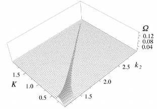
Figure 1: Growth-rate as a function of nondimensional wave-number $k_{2}$ and perturbation $K$ for $\tilde{A}=\tilde{B}=0.2$ and $k_{1}=1$. Axes are in nondimensional units.

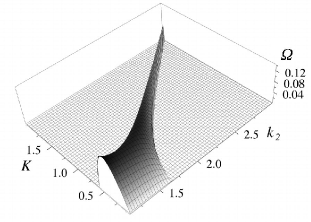
Figure 2: Growth-rate as a function of nondimensional wave-number $k_{2}$ and perturbation $K$ for $\tilde{A}=\tilde{B}=0.4$ and $k_{1}=1$. Axes are in nondimensional units.

We then compute the largest imaginary solution of the polynomial function $\Omega$ and plot it as a surface for different values of $k_{2}$ and perturbation $K$; as $k_{2}$ is increased, the amplitude $\tilde{B}$ is kept constant. In dimensional variables this would correspond to increasing the wave-number $k_{2}$ and at the same time maintaining constant its Ursell number.

In Fig. 1 we show the instability region for $\tilde{A}=0.2$, $\tilde{B}=0.2$. The plot clearly exhibits an unstable region with a growth-rate different from zero. Note that on the horizontal axes $k_{2}$ starts from values slightly larger than 1, because, as has been previously stated, the CNLS system that we have derived is not valid when $k_{2}\simeq k_{1}$. In Fig. 2 we show the same diagram as in Fig. 1, with larger values of the amplitudes $\tilde{A}=0.4$ and $\tilde{B}=0.4$. The instability and the growth-rate have now both increased. We recall that the amplitudes $\tilde{A}$ and $\tilde{B}$ have been scaled by a combination of the steepness, of the nonlinear and dispersive parameters, respectivelly $\mu$ and $\lambda$, of the KdV equation. From a physical point of view, increasing the amplitude $\tilde{A}$ or $\tilde{B}$ implies an increase of the nonlinearity of the wave system that can be achieved for example also by a decrease in the water depth. As the the water depth decreases the instability region and the growth-rate increase and therefore, double-peak spectra are more likely to evolve naturally into single-peak spectra which are stable in shallow water. Results can be summarized as follows: in shallow water the dynamics of two wave trains can be unstable; as expected the growth-rate and the size of the instability region depend on the nonlinearity of the system.

The derived CNLS system represents a very crude simplification of the real problem: effects related to a non constant water depth could be considered; directionality could also be simply included by applying the multiple-scale method to the Kadomtsev-Petviashvili equation ABLSEG (an extension of the KdV equation that includes the dynamics of transverse perturbations); higher order effects could also be investigated.

We believe that the present work offers new perspectives for understanding the dynamics of double-peaked spectra in shallow water. Accurate comparison with experiments and numerical simulations are definitely needed in order to validate the obtained theoretical results. As a final remark we would like to stress that we have started the derivation of the CNLS equations from the KdV; the Inverse Scattering theory furnishes a unique method for investigating all its solutions. It would be therefore interesting to interpret the unstable solutions of the CNLS equations in terms of the Inverse Scattering modes for the KdV equation.

Acknowledgements M.O. is grateful to J.M. Smith for pointing out the problem. This work was supported by the O.N.R., USA. Torino University funds (60 %) are also acknowledged. D. Resio is acknowledged for support and valuable discussions.

References

- (1) E. F. Thompson, “Energy spectra in shallow U.S. coastal waters,” Tech. Paper No. 82-2, Coast. Engrg. Res. Ctr., U.S. Army Corps of Engrs., Fort Belvoir, Va (1980).
- (2) J. M. Smith and C. L. Vincent, “Shoaling and decay of two wave trains on a beach, ” J. Wtrways., Port, Coast. and Oc. Engrg., 118 517-533, (1992).
- (3) Y. Chen, R. T. Guza and S. Elgar, “Modelling spectra of breaking surface waves in shallow water,” J. Geophys. Res. 102, 25,035-25,046 (1997).
- (4) M. J. Ablowitz and H. Segur, Solitons and Inverse Scattering Transform, SIAM, Philadelphia, PA (1981).
- (5) C. C. Mei, The Applied Dynamics of Ocean Surface Waves John Wiley Sons, (1993).
- (6) A. R. Osborne and M. Petti, “Laboratory-generated, shallow water surface waves: Analysis using the periodic, inverse scattering transform,” Phys. of Fluids 6, 1727-1744 (1994).
- (7) A. R. Osborne, E. Segre, G. Boffetta and L. Cavaleri, “Soliton basis states in shallow-water ocean surface waves,” Phys. Rev, Lett. 67, 592-595 (1991).
- (8) A. R. Osborne, M. Serio, L. Bergamasco and L. Cavaleri, “Solitons, cnoidal waves and nonlinear interactions in shallow-water ocean surface waves,” Physica D 123, 64-81 (1998).
- (9) B. Whitham, Linear and nonlinear waves (J. Wiley and Sons, 1973).
- (10) N. J. Zabusky and M. D. Kruskal, “Interaction of solitons in a collisionless plasma and the recurrence of initial states,” Phys. Rev. Lett. 15, 240-243 (1965)
- (11) R.Grimshaw, D.Pelinovsky, E. Pelinovsky and T. Talipova, “Wave group dynamics in weakly nonlinear long-wave models,” Physica D 159 35-57, (2001).
- (12) C.R. Menyuk, “Nonlinear pulse propagation in birefringent optical fibers,” IEEE J. Quantum Electron. QE-23 174-176 (1987).
- (13) C.R. Menyuk, “Pulse propagation in an elliptically birefringent Kerr medium,” IEEE J. Quantum Electron. 25 2674-2682 (1989).
- (14) S.V. Manakov, “On the theory of two-dimensional stationary self-focusing of electromagnetic waves,” Sov. Phys.-JETP, 38 248-253 (1974).
- (15) H. Hashimoto and H. Ono, “Nonlinear modulation of gravity wave,” J. Phys. Soc. Japan 33, 805-811 (1972).
- (16) V.E. Zakharov and E.A. Kuznetsov, “Multi-scale expansion in the theory of systems integrable by the inverse scattering transform,” Physica D 32, 455-463 (1986).
- (17) E.R. Tracy, J.W. Larson, A.R. Osborne and L. Bergamasco “On the nonlinear Schroedinger equation limit of the Korteweg-de Vries equation,” Physica D 18, 83-106 (1988).
- (18) M.G. Forest, D.W. McLaughlin, D.J. Muraki and O.C. Wright, “Nonfocusing Instability in Coupled, Integrable Nonlinear Schrödinger pdes,” J. Nonlinear Sci. 10, 291-331, (2000).
- (19) G.J Roskes, “Nonlinear multiphase deep-water wavetrains,” Phys of Fluids 19, 1253-1254 (1976).
- (20) M. Okamura, “Instability of weakly nonlinear standing gravity waves,” J. Phys. Soc. Jpn. 53, 3788 (1984).
- (21) R.D. Pierce and E. Knobloch, “On the modulational stability of travelling and standing water waves,” Phys. of Fluids 6, 1177 (1994).