Chaos and flights in the atom-photon interaction in cavity QED

Abstract

We study dynamics of the atom-photon interaction in cavity quantum electrodynamics (QED), considering a cold two-level atom in a single-mode high-finesse standing-wave cavity as a nonlinear Hamiltonian system with three coupled degrees of freedom: translational, internal atomic, and the field. The system proves to have different types of motion including Lévy flights and chaotic walkings of an atom in a cavity. It is shown that the translational motion, related to the atom recoils, is governed by an equation of a parametric nonlinear pendulum with a frequency modulated by the Rabi oscillations. This type of dynamics is chaotic with some width of the stochastic layer that is estimated analytically. The width is fairly small for realistic values of the control parameters, the normalized detuning $\delta$ and atomic recoil frequency $\alpha$. It is demonstrated how the atom-photon dynamics with a given value of $\alpha$ depends on the values of $\delta$ and initial conditions. Two types of Lévy flights, one corresponding to the ballistic motion of the atom and another one corresponding to small oscillations in a potential well, are found. These flights influence statistical properties of the atom-photon interaction such as distribution of Poincaré recurrences and moments of the atom position $x$. The simulation shows different regimes of motion, from slightly abnormal diffusion with $<x^{2}>\sim\tau^{1.13}$ at $\delta=1.2$ to a superdiffusion with $<x^{2}>\sim\tau^{2.2}$ at $\delta=1.92$ that corresponds to a superballistic motion of the atom with an acceleration. The obtained results can be used to find new ways to manipulate atoms, to cool and trap them by adjusting the detuning $\delta$.

I Introduction

Cavity quantum electrodynamics is a rapidly developing field of physics studying the interaction of atoms with photons in high-finesse cavities in a wide range of electromagnetic spectrum, from microwaves to visible light, in such conditions under which both atoms and fields may manifest their quantum nature (for reviews on quantum and atom optics, see B ; ASM ). Modern experiments in cavity QED have achieved the exceptional circumstance of strong atom-field coupling for which the strength of the coupling exceeds both the atomic dipole decay and the cavity field decay providing manipulations with single atoms and photons Y99 ; HLD ; EMK ; MF99 ; PFM . Trapped atoms and ions, interacting with laser fields in the regime of the strong coupling, have been used not only to study fundamentals of quantum mechanics W98 ; MM96 but also for applications in the rapidly growing fields of quantum computing, quantum communication (see, for example, CZ95 ; MM95 ), quantum chaos Z81 ; H91 , and decoherence Z91 ; GJ96 .

A special comment should be related to the notion of chaos that we use in the paper. The real system is quantum and the quantum chaos per se does not exist. The notion “quantum chaos” just refers to the behavior of quantum systems whose classical counterparts behave chaotically. Through the paper the notion “chaos” will be used only in that meaning since all our consideration will be semiclassical. The key issue of quantum chaos is the correspondence between the classical and quantum pictures of chaotic dynamics. Chaotic dynamics in the atom-photon physics appeared in the paper Haken , where the semiclassical model of a single-mode, resonant, and homogeneously broadened laser, considered as an open dissipative system, has been shown to be equivalent to a Lorentz-type strange attractor, and the paper BZT , where Hamiltonian semiclassical chaos has been shown to arise in the Dicke model with non-resonant terms describing the interaction of an ensemble of identical two-level atoms with their own radiation field in an ideal resonant cavity. The fully quantum version of the latter model has been considered in BBZ . It was shown in [18] that in a parameter range, corresponding to classical chaos, the evolution of the system becomes essentially quantum after the so-called “breaking time” $\tau_{\hbar}$ BZ78 which obeys in this regime the logarithmic law $\tau_{\hbar}\sim\lambda^{-1}\ln({\rm const}/\hbar)$, where $\lambda$ is the maximal Lyapunov exponent. All results presented here as chaotic dynamics are valid up to $t\lesssim\tau_{\hbar}$.

The physical mechanism of semiclassical chaos in the Dicke model is tied to virtual transitions which are described by non-resonant (or counter-rotating) terms in the Dicke Hamiltonian. They are small under usual conditions. Trying to find another mechanism of local instability in the Hamiltonian atom-photon dynamics without pump and losses, the authors of PK97 ; PKK99 proposed the semiclassical model with atoms moving through a standing-wave cavity in a direction along which the cavity sustains a space-periodic field. The standing wave modulates the atom-field coupling providing in a certain range of the system’s parameters intermittent Rabi oscillations. Another way to change the atom-field coupling is modulating the cavity length, studied in IKP . New effects in the model with moving atoms may arise beyond the simple semiclassical approximation. Chaotic vacuum Rabi oscillations, a new kind of reversible spontaneous emission, have been shown P00 ; PK00 to occur in the model with interatomic quantum correlations.

Experiments to study the quantum dynamics of classically chaotic systems for the atom-photon interaction in cavities and traps have been intensively studied with cold atoms in a phase-modulated standing wave MR94 and in an amplitude-modulated standing wave HT (following to the proposition of GSZ ), and in a pulsed standing wave MR95 ; AG . Cold sodium or cesium atoms, which are kicked by a periodically pulsed standing wave of far-detuned light, is an excellent experimental realization of a paradigm model of quantum chaos, a $\delta$-kicked quantum rotor. Dynamical localization, that was observed in the atomic momentum distribution, is the quantum suppression of the classical momentum diffusion. A typical underlying phase-space structure of classical chaotic systems consists of stochastic webs, islands, and chains of islands embedded in the stochastic sea. The chaotic motion occupies a certain area in phase space. Because of islands and their boundaries, typical behavior of chaotic systems can be intermittent with long (quasi)regular oscillations (the so-called Lévy flights) interrupted by the chaotic pieces of trajectories. This intermittency leads to the anomalous diffusion with Lévy distribution functions or a similar one, which have power-wise tails (for reviews on Lévy processes in physics see SZK , where the term “strange kinetics” was coined, and Z98 ). It was found with kicked cold cesium atoms K0 that for certain pulses amplitudes, where the respective classical analog may exhibit anomalous diffusion, the momentum distributions were not exponentially localized for the time of observation (see also BS99 ; AI99 ; RA01 ). It should be mentioned that anomalous diffusion and Lévy flights have been even earlier found with cold atoms and employed in a subrecoil laser cooling scheme BB94 ; RB95 ; SL99 .

In experiments with $\delta$-kicked atoms, the detuning between the optical and atomic transition frequencies is large (relative to the natural line-width), so the probability is small to find an atom, initially prepared in the ground state, in the excited state, and the excited state amplitude can be adiabatically eliminated GSZ . In this approximation, an effective Hamiltonian is that of a driven nonlinear oscillator with 3/2 degrees of freedom. Generally speaking, the atom-photon interaction in a high-finesse cavity is, mainly, the interaction between internal (electronic) and external (motional) atomic degrees of freedom and the cavity field. A corresponding one-dimensional model, including the interaction of all those degrees of freedom, has been introduced in papers PK01 ; PS01 in the context of Hamiltonian chaos. In this paper, we use a slightly generalized version of that model with three degrees of freedom to study the effects of chaos and Lévy flights in the strongly-coupled atom-field system.

In Sec. II the semiclassical basic equations in the Heisenberg representation are derived in the form of six coupled nonlinear equations with two control parameters, the normalized detuning $\delta$ and atomic recoil frequency $\alpha$. Taking into account that the frequency of the atomic (and field) Rabi oscillations is much more larger than the frequency of translational oscillations, reduced Bloch-like equations of the atom-field internal motion are derived and solved in Sec. III. The motion of the center of the atom mass is governed by a single equation of a parametrically perturbed pendulum. This dynamics generates a stochastic layer with an exponentially small width. In Sec. IV we simulate the basic set of equations at the fixed value of the normalized recoil frequency $\alpha=10^{-3}$ corresponding to a light atom in a microcavity with realistic parameters Y99 ; HLD ; EMK ; MF99 ; PFM . The maximal Lyapunov exponents and Poincaré sections are calculated and it is found that the detuning $\delta$ is a crucial parameter in transition to chaos. Statistical properties of the atom-photon interaction are considered in Sec. V. We give an evidence of two types of Lévy flights of an atom, one corresponding to an almost linear dependence of the atomic position $x$ on time (superdiffusive and superballistic regime), and another one corresponding to small regular oscillations of the atom in the potential well. The Lévy flights influence strongly such statistical properties of atoms and photons as distribution of Poincaré recurrences and moments of $x$. The distribution of recurrences and time-evolution of the moments depend on the value of the detuning $\delta$ demonstrating different regimes from an almost normal diffusion to a superdiffusion. In Sec. VI we discuss briefly ways to manipulate the atomic motion by varying control parameters and initial internal atomic states. It is possible, in particular, to cool and trap atoms by adjusting the detuning.

II Basic equations

The basic model of interaction of radiation with matter describes the energy exchange between a two-level atom and a single mode of the quantized radiation field in an ideal lossless cavity JC . In general, this interaction should involve not only the internal atomic transitions and field states but also the center-of-mass motion of the atom. With the recoil effect to be included into consideration, the standard Jaynes-Cummings Hamiltonian can be extended as follows:

$$H=\frac{\hat{p}^{2}}{2m}+\hbar\omega_{a}\hat{s}_{z}+\hbar\omega_{f}\hat{a}^{+}\hat{a}-\hbar\Omega_{0}(\hat{a}^{+}\hat{s}_{-}+\hat{a}\hat{s}_{+})\cdot\cos k_{f}\hat{x}\ ,$$ (1)

where $\hat{x}$ and $\hat{p}$ are the atomic position and momentum operators, respectively. Transitions between two electronic states, separated by the energy $\hbar\omega_{a}$, are described by the spin operators with the commutation relations, $[\hat{s}_{+},\hat{s}_{-}]=2\hat{s}_{z}$ and $[\hat{s}_{z},\hat{s}_{\pm}]={\pm}\hat{s}_{\pm}$. The photon annihilation and creation operators with the commutation rule $[\hat{a},\hat{a}^{+}]=1$ characterize a selected mode of the radiation field of the frequency $\omega_{f}$ and the wave number $k_{f}$ in a lossless cavity of the Fabry-Perot type. The parameter $\Omega_{0}$ is the amplitude value of the atom-field dipole coupling which depends on the position of an atom inside a cavity. As it is usually adopted in cavity QED, we write down the Heisenberg equations for the external atomic operators, $\hat{x}$ and $\hat{p}$, and for slowly-varying amplitudes of the field and spin operators $\hat{a}(t)=\hat{a}\exp(-i\omega_{f}t),\quad\hat{a}^{+}(t)=\hat{a}^{+}\exp(i\omega_{f}t),\quad\hat{s}_{\pm}(t)=\hat{s}_{\pm}\exp(\pm i\omega_{f}t)$ and $\hat{s}_{z}(t)=\hat{s}_{z}$

$$\begin{array}[]{lll}\frac{d}{dt}\hat{x}=\frac{\hat{p}}{m}\ ,\\ \frac{d}{dt}\hat{p}=-\hbar k_{f}\Omega_{0}(\hat{a}^{+}\hat{s}_{-}+\hat{a}\hat{s}_{+})\sin k_{f}\hat{x}\ ,\\ \frac{d}{dt}\hat{s}_{+}=-i(\omega_{f}-\omega_{a})\hat{s}_{+}+2i\Omega_{0}\hat{a}^{+}\hat{s}_{z}\cos k_{f}\hat{x}\ ,\\ \frac{d}{dt}\hat{s}_{-}=i(\omega_{f}-\omega_{a})\hat{s}_{-}-2i\Omega_{0}\hat{a}\ \hat{s}_{z}\cos k_{f}\hat{x}\ ,\\ \frac{d}{dt}\hat{s}_{z}=-i\Omega_{0}(\hat{a}^{+}\hat{s}_{-}-\hat{a}\hat{s}_{+})\cos k_{f}\hat{x}\ ,\\ \frac{d}{dt}\hat{a}^{+}=-i\Omega_{0}\hat{s}_{+}\cos k_{f}\hat{x}\ ,\\ \frac{d}{dt}\hat{a}=i\Omega_{0}\hat{s}_{-}\cos k_{f}\hat{x}\ .\end{array}$$ (2)

To avoid cumbersome notations in Eqs. (2) we use for the amplitudes the same notations as for the respective whole operators.

In order to derive a tractable closed set of equations for expectation values from the Heisenberg operator equations (2), we use the semiclassical approximation. It means that all the operators and their products in Eqs. (2) are averaged over an initial quantum state, which is supposed to be a product state of the translational, electronic, and field states. The expectation values of all the operator products are factorized to the products of the respective expectation values, e.g., $\langle(\hat{a}^{+}\hat{s}_{-}+\hat{a}\hat{s}_{+})\cdot\sin k_{f}\hat{x}\rangle$ $=(\langle\hat{a}^{+}\rangle\langle\hat{s}_{-}\rangle+\langle\hat{a}\rangle\langle\hat{s}_{+}\rangle)\sin(k_{f}\langle\hat{x}\rangle)$. By choosing the following dimensionless expectation values: $x=k_{f}\langle\hat{x}\rangle$, $p=\langle\hat{p}\rangle/\hbar k_{f}$, $a_{x}=\frac{1}{2}\langle\hat{a}+\hat{a}^{+}\rangle$, $a_{y}=\frac{1}{2i}\langle\hat{a}-\hat{a}^{+}\rangle$, $s_{x}=\frac{1}{2}\langle\hat{s}_{-}+\hat{s}_{+}\rangle$, $s_{y}=\frac{1}{2i}\langle\hat{s}_{-}-\hat{s}_{+}\rangle$, as dynamical variables, we finally get from Eqs. (2) a nonlinear dynamical system

$$\begin{array}[]{lll}\dot{x}=\alpha p\ ,\\ \dot{p}=-2(a_{x}s_{x}+a_{y}s_{y})\sin x\ ,\\ \dot{s}_{x}=-\delta s_{y}+2a_{y}s_{z}\cos x\ ,\\ \dot{s}_{y}=\delta s_{x}-2a_{x}s_{z}\cos x\ ,\\ \dot{a}_{x}=-s_{y}\cos x\ ,\\ \dot{a}_{y}=s_{x}\cos x\ ,\end{array}$$ (3)

that describes the interaction between three degrees of freedom in the strongly coupled atom-field system, translational $(p,x)$, electronic $(s_{x},s_{y})$, and the field $(a_{x},a_{y})$ ones. The dot in Eqs. (3) denotes the derivative with respect to the normalized time $\tau=\Omega_{0}t$. The control parameters are the normalized recoil frequency $\alpha=\hbar k_{f}^{2}/m\Omega_{0}$ and the normalized detuning between the frequencies of the field mode and the electronic transition, $\delta=(\omega_{f}-\omega_{a})/\Omega_{0}$. The system (3) conserves the energy

$$W=\frac{\alpha}{2}p^{2}-2(a_{x}s_{x}+a_{y}s_{y})\cos x-\delta s_{z}\ ,$$ (4)

and it possesses two additional first integrals

$$s_{x}^{2}+s_{y}^{2}+s_{z}^{2}=S^{2},\quad a_{x}^{2}+a_{y}^{2}+s_{z}=N\ .$$ (5)

The first one is simply the conservation of the atomic probability, and the second one is a conserved total number of excitations, which is known to be a constant in the rotating-wave approximation. The equation of motion for the atomic inversion $s_{z}$ is easily derived with the help of the integral $N$

$$\dot{s}_{z}=2(a_{x}s_{y}-a_{y}s_{x})\cos x\ .$$ (6)

The semiclassical approximation, we used for (3), means that the atom as a classical particle with external and internal states moves in a self-consistent classical radiation field.

From the dynamical systems point of view equations (3) represent a system with 3 degrees of freedom (one degree of freedom per a canonically conjugate pair of the generalized momentum and coordinate) in 6-dimensional phase space. Indeed, we reinsert Eq.(6) for $\dot{s}_{z}$ into (3). After that the system (3) describes 3 degrees of freedom: the atom external coordinates ($x,p$), the atom internal coordinates ($s_{x},s_{y}$), and the field coordinates ($a_{x},a_{y}$). There are 2 constrains: energy integral $E=H(p,x;s_{x},s_{y};a_{x},a_{y})$ and the spin integral $S$. The number of excitations $N$ should be used to determine $s_{z}$ as a function of other variables. That means that full dynamics is defined in 4-dimensional hyperspace and should have domains of chaos due to its nonintegrability. One can say that the location of the domains of chaotic motion, islands of regular dynamics, set of stationary points, and boundaries define a topology of the system’s flow. The topology is two-parametric $(E,S)$ and very complicated. Its description needs a separate investigation.

III Reduced dynamics and the estimation of the stochastic layer width

We can simplify further the basic equations (3) introducing the combined atom-field variables

$$u=2(a_{x}s_{x}+a_{y}s_{y}),\quad v=2(a_{y}s_{x}-a_{x}s_{y})$$ (7)

and using the integrals (5). As a result, one arrives at the closed five-dimensional dynamical system

$$\begin{array}[]{lll}\dot{x}=\alpha p\ ,\\ \dot{p}=-u\sin x\ ,\\ \dot{u}=\delta v\ ,\\ \dot{v}=-\delta u+2(2Ns_{z}-3s_{z}^{2}+S^{2})\cos x\ ,\\ \dot{s}_{z}=-v\cos x\ ,\end{array}$$ (8)

which generalizes the corresponding equations of the paper PS01 (see Eqs. (3) therein which were derived in the limit of large $N$). It is obvious from Eqs. (8) that at exact resonance, $\delta=0$, the slow translational variables $x$ and $p$ are separated from the fast atom-field $u,v$, and $s_{z}$, and the system (8) becomes integrable. At $\delta=0$, the atom moves in a spatially periodic optical potential $U=-u(0)\cos x$ with $u(0)=u(\tau=0)$ = const, and its center-of-mass motion satisfies the pendulum equation $\ddot{x}+\alpha u(0)\sin x=0$. It is easy to find that the dynamics of the internal atomic variable $s_{z}$ satisfies the following equation:

$$\dot{s}_{z}=\pm 2\sqrt{s_{z}(s_{z}^{2}-Ns_{z}-S^{2})+C}\ \cos x\ ,$$ (9)

where $C$ is an integration constant, and $x(\tau)$ is a solution of the pendulum equation mentioned above. The equation (9) can be integrated in terms of elliptic Jacobian functions with a solution which converges to the well-known Jaynes-Cummings semiclassical solution JC in the limit $x$ = const.

Out of resonance, at $\delta\neq 0$, the system (8) exhibits chaotic dynamics. In order to clarify the origin of chaos, consider Eqs. (8) in the limit of large number of excitation $N$ and large detunings $\delta$ comparing to $S^{2}$. Taking into account that the normalized Rabi frequency is of the order of $\sim\sqrt{N}>1$ and is much more larger than the frequency of small translational oscillations, $\sqrt{\alpha}\ll 1$, the equations for the fast atom-field oscillations are reduced to the Bloch-like form

$$\begin{array}[]{lll}\dot{u}=\delta v\ ,\\ \dot{v}=-\delta u+4Ns_{z}\cos x\ ,\\ \dot{s}_{z}=-v\cos x\ ,\end{array}$$ (10)

where the function $\cos x$ may be considered approximately as a constant $c$ over a period of time of many Rabi oscillations. In this approximation, the quantity

$$u^{2}+v^{2}+N(2s_{z})^{2}=R$$ (11)

plays a role of the length of Bloch vector, and the general solution of the Bloch-like equations (10) can be found

$$u=u(0)\left[N\left(\frac{2c}{\Omega_{N}}\right)^{2}+\left(\frac{\delta}{\Omega_{N}}\right)^{2}\cos\Omega_{N}\tau\right]+\\ +\frac{\delta}{\Omega_{N}}v(0)\sin\Omega_{N}\tau+\frac{4N\delta c}{\Omega_{N}^{2}}s_{z}(0)(1-\cos\Omega_{N}\tau)\ ,$$

$$v=-\frac{\delta}{\Omega_{N}}u(0)\sin\Omega_{N}\tau+v(0)\cos\Omega_{N}\tau+\\ +\frac{4Nc}{\Omega_{N}}s_{z}(0)\sin\Omega_{N}\tau\ ,$$ (12)

$$s_{z}=u(0)\frac{c\delta}{\Omega_{N}^{2}}(1-\cos\Omega_{N}\tau)-\frac{c}{\Omega_{N}}v(0)\sin\Omega_{N}\tau+\\ +s_{z}(0)\left[\left(\frac{\delta}{\Omega_{N}}\right)^{2}+N\left(\frac{2c}{\Omega_{N}}\right)^{2}\cos\Omega_{N}\tau\right]\ ,$$

where the quantity

$$\Omega_{N}=\sqrt{\delta^{2}+(2c)^{2}N}$$ (13)

is similar to the Rabi frequency.

Since the function $\cos x$ varies in time slowly comparing to the fast oscillating $u,v$, and $z$, the atom-field variable $u$ may be considered approximately as a spatially independent frequency- and amplitude-modulated signal that parametrically excites the translational motion:

$$\ddot{x}+\alpha u(\tau)\sin x=0\ ,$$ (14)

that follows from the first two equations of the system (8). The modulation has especially simple form for initial conditions $u(0)=v(0)=0$ and $s_{z}(0)=\mid S\mid$, that corresponds to the atom prepared initially in the upper state while the field may be initially at any state, and $c=1$:

$$u(\tau)=\frac{4N\delta\mid S\mid}{\Omega_{N}^{2}}(1-\cos\Omega_{N}\tau)\ .$$ (15)

The Eq. (14) is derived from the following effective classical Hamiltonian

$${\cal H}=\frac{1}{2}\dot{x}^{2}-\omega^{2}\cos x+\omega^{2}\cos\Omega_{N}\tau\cdot\cos x={\cal H}_{0}+V\ ,$$ (16)

where ${\cal H}_{0}$ is the unperturbed Hamiltonian of a free pendulum with the following frequency of small oscillations:

$$\omega=\frac{2}{\Omega_{N}}\sqrt{\alpha N\mid\delta\mid\ \mid S\mid}\ .$$ (17)

Rewriting the perturbation $V=\omega^{2}\cos\Omega_{N}\tau\cdot\cos x$ in the form

$$V=\frac{\omega^{2}}{2}\left[\cos(x+\Omega_{N}\tau)+\cos(x-\Omega_{N}\tau)\right]\ ,$$ (18)

one may consider (16) as the Hamiltonian of a particle moving in the field of three plane waves in a frame moving with the phase velocity of the first wave, while the phase velocities of the second and third waves are $\Omega_{N}$ and $-\Omega_{N}$, respectively.

As it follows from the general theory of perturbed motion of Hamiltonian systems with 3/2 degrees of freedom ZS91 , the Hamiltonian (16) induces chaotic dynamics in the so-called stochastic layer that appears due to the separatrix splitting. Let us consider the motion in the neighborhood of unperturbed separatrix of the pendulum (16). Consider the Poincaré-Melnikov integral

$$\Delta E=\int_{-\infty}^{\infty}\{{\cal H}_{0},V\}d\tau=\\ =\omega^{2}\int_{-\infty}^{\infty}\dot{x}\sin(x-\Omega_{N}\tau)d\tau\ ,$$ (19)

where $\{{\cal H}_{0},V\}$ is the Poisson bracket. This integral describes changes of the atomic translational energy at the separatrix ${\cal H}_{0}=E_{s}=\omega^{2}$. To estimate (19) for the dynamics near the separatrix, one can use for $x$ and $\dot{x}$ their known unperturbed separatrix solutions

$$\begin{gathered}x_{s}=4\ {\rm arctan}\exp[\pm\omega(\tau-\tau_{n})]\ ,\\ \dot{x}_{s}=\pm\frac{2\omega}{\cosh[\omega(\tau-\tau_{n})]}\ ,\end{gathered}$$ (20)

where $\tau_{n}$ is introduced as an initial condition. Using the solutions (20), we get

$$\Delta E_{n}=\pm 2\omega^{2}\int_{-\infty}^{\infty}\frac{dt}{\cosh t}\sin\left(x-\frac{\Omega_{N}}{\omega}t-\phi_{n}\right),$$ (21)

where the new time $t=\omega(\tau-\tau_{n})$ and phase $\phi_{n}=\Omega_{N}\tau_{n}$ were introduced. The integral (21) has been calculated to give

$$\Delta E_{n}=\Delta E_{s}\sin\phi_{n}\ ,$$ (22)

$$\Delta E_{s}=2\pi\ \Omega_{N}^{2}\frac{\exp(\pi\Omega_{N}/2\omega)}{\sinh(\pi\Omega_{N}/\omega)}\ .$$ (23)

The oscillating function $\Delta E_{n}$ has simple zeroes that implies transversal intersections of stable and unstable heteroclinic manifolds of saddle points known as a complicated heteroclinic structure. On the basis of general properties of motion near the separatrix, the separatrix map can be introduced ZS91 .

$$E_{n+1}=E_{n}+\Delta E_{s}\sin\phi_{n}\ ,$$ (24)

$$\phi_{n+1}=\phi_{n}+\frac{\Omega_{N}}{\omega}\ln\frac{32E_{s}}{|E_{n+1}-E_{s}|}\ .$$ (25)

The condition

$$K=\max\left|\frac{\delta\phi_{n+1}}{\delta\phi_{n}}-1\right|\simeq\\ \simeq\frac{2\pi\Omega_{N}^{3}}{\omega}\ \frac{\exp(\pi\Omega_{N}/2\omega)|\sin\phi_{n}|}{|E_{n+1}-E_{s}|\sinh(\pi\Omega_{N}/\omega)}\gtrsim\ 1$$ (26)

defines the stochastic layer width which can be estimated in the case of the large parameter $\Omega_{N}/\omega\gg 1$ (see the respective estimations with real atoms in the concluding section) as follows:

$$\delta E_{s}\equiv|E_{n+1}-E_{s}|\lesssim\frac{8\pi\Omega_{N}^{3}}{\omega}\exp\left(-\frac{\pi\Omega_{N}}{2\omega}\right).$$ (27)

The dimensionless width of the stochastic layer is finally given by

$$\frac{\delta E_{s}}{\omega^{2}}\simeq 8\pi\left(\frac{\Omega_{N}}{\omega}\right)^{3}\exp\left(-\frac{\pi\Omega_{N}}{2\omega}\right)\ ,$$ (28)

where the large parameter

$$\frac{\Omega_{N}}{\omega}=\frac{\delta^{2}+4N}{2\sqrt{\alpha N\mid\delta\mid\ \mid S\mid}}$$ (29)

under the conditions $N,\delta\gg\mid S\mid\simeq 1$ and $\delta^{2}\ll 4N$ is estimated as

$$\frac{\Omega_{N}}{\omega}\simeq 2\sqrt{\frac{N}{\alpha\mid\delta\mid}}\ .$$ (30)

For the considered case the width of the stochastic layer of the reduced atom-field dynamics is exponentially small in (28), multiplied by a large parameter. Due to (30) the final width depends on the control parameters $N$, $\alpha$ and $\delta$, and the formula (28) is useful in estimating the ranges of the control parameters where one may expect chaotic motion.

The estimation (28) provides the lower bound for the the width of the stochastic layer that appears due to the simplest harmonic modulation (15). Small changes in energy produce comparatively small changes in frequency of oscillations. Nearby the bottom of potential wells and high over potential hills (where the energy is much less and much greater than $E_{s}$), small changes in frequency give rise to respectively small changes in phase during the period of oscillations. Nearby the unperturbed separatrix, where the period goes to infinity, even small changes in frequency lead to dramatic changes in phase. This is the reason of exponential instability of the parametric oscillator (14) and (15) which models chaotic motion of the atom moving through a periodic standing wave.

IV Lyapunov exponents and Poincaré sections

In this section, we present numerical simulations with the basic set of equations (3) and the integrals of motion (4) and (5) with $S^{2}=3/4$ (the actual value of $S^{2}$ has no importance since it always can be renormalized to 1) and $N=10$. The system (3) has two control parameters, the normalized detuning $\delta$ between the atomic transition and cavity frequencies and the normalized recoil frequency $\alpha$. As it will be estimated in the concluding section, $\alpha$ is in the range from $10^{-5}$ to $10^{-2}$ for real atoms. We choose $\alpha=10^{-3}$ in simulations throughout the paper.

Figure 1: The maximal Lyapunov exponent $\lambda$ in units of the maximal atom-field coupling rate $\Omega_{0}$ versus the atom-field detuning $\delta$ in units $\Omega_{0}$. (a) $s_{z}(0)=-0.863$. (b) $s_{z}(0)=0$. (c) $s_{z}(0)=0.863$.

a                                             c

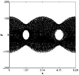
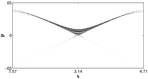
        b                                             d

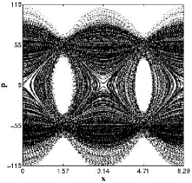
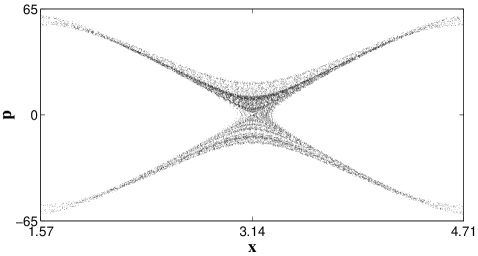
Figure 2: Projections of the Poincaré sections on the plane of the atomic momentum $p$ in units $\hbar k_{f}$ and the position in units of $k_{f}^{-1}$. (a) $s_{z}(0)=-0.8660254$ and $\delta=1.2$. (b) $s_{z}(0)=-0.863$ and $\delta=1.2$. (c) $s_{z}=-0.8660254$, $\delta=1.92$, and $p(0)=2.1$ in all the above fragments. (d) $s_{z}=-0.863$, $\delta=1.92$, and $p(0)=20$. $x,p$ are dimensionless.

The detuning $\delta$, as it was shown in PK01 ; PS01 , is the crucial parameter in transition to chaos in the atom-field system with the center-of-mass motion. It is obvious from the set (8), which is equivalent to the basic one (3), that at exact resonance, $\delta=0$, the motion is regular. At large detunings, $\delta\gg N$, the motion is expected to be quasiregular since the nonlinear term in the fourth equation of the set (8) is small, compared to the linear term of the same equation. With far-detuned light, one does not expect pronounced atomic Rabi oscillations. In order to find the range of the detunings, where the motion is expected to be chaotic, we compute the dependence of the maximal Lyapunov exponent $\lambda$ on the detuning $\delta$.

Lyapunov exponents characterize the behavior of close trajectories in phase space. Consider a trajectory, some sequence of time instants $\tau_{0}$, $\tau_{1}$, $\tau_{2}$, … with equal intervals $\Delta\tau$, and a ball around the initial point of the trajectory. Lyapunov numbers $\Lambda_{j}$ ($j=1,...,M$; M is a number of variables) show per-interval $\Delta\tau$ changes of the axes of the “ellipsoid” of the deformed ball ASY . In our case $M=6$ after exclusion of $s_{z}$. The $k$-th Lyapunov exponent is defined as $\lambda_{k}=\ln\Lambda_{k}$. Typically $\Lambda_{k}$ depends on time and $\lambda_{k}$ should be replaced by their mean values ASY . In Hamiltonian systems, due to the phase volume conservation, $\Lambda_{1}\cdot\Lambda_{2}\cdot...\cdot\Lambda_{M}=1$ and $\lambda_{1}+...+\lambda_{M}=0$. For integrable system all $\Lambda_{k}$ are pure imaginary and they make pairs: $\lambda_{2}=-\lambda_{1}$, $\lambda_{4}=-\lambda_{3}$, $\lambda_{6}=-\lambda_{5}$, since the number $M$ of equations is even. This result follows from the so-called Liouville-Arnold theorem A88 . In our case, for the reduced system of 6 variables ($p,x;a_{x},a_{y};s_{x},s_{y}$) and two constrains (integrals of motion), we have two imaginary pairs, say $\lambda_{1,2}=\pm i\sigma_{1}$, $\lambda_{3,4}=\pm i\sigma_{2}$ ($\sigma_{1,2}$ real), and $\lambda_{5}$, $\lambda_{6}$ that satisfy the condition $\lambda_{5}+\lambda_{6}=0$, and therefore $\Lambda_{5}\cdot\Lambda_{6}=1$, i.e. $\Lambda_{6}=1/\Lambda_{5}$. The chaos means that $\lambda_{5,6}$ are real LL ; ASY . If, say $\Lambda_{5}<1$ ($\lambda_{5}<0$), then $\Lambda_{6}>1$ ($\lambda_{6}>0$) and $\lambda_{6}$ is called maximal Lyapunov exponent. It has a nice physical meaning: the maximal Lyapunov exponent measures a rate of the separation of initially close trajectories, and typically for the practical goal, the mean value $\lambda=\overline{\lambda_{6}}$ over time is used. To compute $\lambda$, we use the standard algorithm LL

$$\lambda=\lim_{n{\rightarrow}\infty}\frac{1}{n}\sum_{k=1}^{n}\ln\frac{\Delta(\tau_{k})}{\Delta(\tau_{k-1})},$$ (31)

where $\Delta(\tau_{k-1})$ is a distance between two close trajectories at time $\tau_{k-1}$, and the value $\Delta(\tau_{k})/\Delta(\tau_{k-1})$ shows the level of separations of the trajectories during the interval $(\tau_{k-1},\tau_{k})$.

In the case that separation doesn’t go exponentially, $\lambda=0$. This happens when $\delta=0$ since the system becomes integrable, and the exponential separation disappears.

The corresponding results of computing maximal Lyapunov exponent $\lambda$ are presented in FIG. 1 with three different initial values of the atomic population inversion $s_{z}(0)=-0.863$; 0; 0.863, respectively. The other initial conditions are the following: $a_{x}(0)=s_{x}(0)=0$, $x(0)=3.14$, $p(0)=2$, and $a_{y}(0)$ and $s_{y}(0)$ are found from the Eqs.(4) and (5) with given $S=\sqrt{3}/2$ and $N=10$. The value $s_{z}(0)=-0.863$ corresponds to the atom initially prepared closely to its ground state for which $s_{z}=-\sqrt{3}/2$. Note that the unusual amplitude values of the atomic population inversion we have are the result of the chosen normalization $S^{2}=3/4$. The atom with $s_{z}(0)=0.863$ is prepared closely to its excited state. In both the cases, the initial components of the transition electric dipole moment, $s_{x}(0)$ and $s_{y}(0)$, are almost zero with $|s_{z}(0)|=0.863$. The atom with $s_{z}(0)=0$ has a maximal electric dipole moment.

As it was expected, at exact resonance $(\delta=0)$, the maximal Lyapunov exponent is exactly equal zero in all the cases assuming a regular motion. As it follows from the results of previous section, a stochastic layer appears with infinitesimally small values of detuning, but its width decreases fast with increasing $\delta$ (see (28) and (29)). We find $\lambda\simeq 0$ with $|\delta|\gtrsim 3$. In physical terms, it means that at exact resonance an atom will periodically exchange excitation with the field, whereas far off resonance its internal states will not (almost) be affected by the field. This interplay results in a maximum of the $\lambda(\delta)$ dependence with almost the same maximal values for $s_{z}(0)=\pm 0.863$ and 0. The results, however, are different in the range $-3\lesssim\delta\lesssim 3$ with different initial values of the population inversion $s_{z}$. It is easy to understand why it is. As it follows from the Bloch-like solution (12) for $s_{z}$, the atom starting, say, in its ground state, $s_{z}(0)=-\sqrt{3}/2$ and $u(0)=v(0)=0$, could reach the upper state $s_{z}=\sqrt{3}/2$ only with $\delta=0$. The same is valid with the other initial values of $s_{z}(0)$: the atom starting with $s_{z}(0)=\sqrt{3}/2$ (or with $s_{z}(0)=0$) will not reach $s_{z}=-\sqrt{3}/2$ (or $s_{z}=\pm\sqrt{3}/2)$ except for the case of exact resonance, $\delta=0$. Thus, the dependencies $\lambda(\delta)$ are different in the range $-3\lesssim\delta\lesssim 3$ with different values of $s_{z}(0)$ in spite of the fact that the maximal Lyapunov exponent is computed over the rather long trajectory.

The model Hamiltonian (1) can be easily generalized to an ensemble of indistinguishable two-level atoms. In the semiclassical approximation, we have not observed any pronounced differences in the strength of chaos (that is characterized by the values of $\lambda$) with different initial internal atomic states. Interatomic quantum correlations, which occur through the mediation of the field generated by the atomic ensemble, have been shown in PK00 (where the model with hot moving atoms but without recoil has been considered) to play a significant role in the atom-field dynamics. Much more strong chaos has been numerically found PK00 in the vacuum Rabi oscillations with atoms initially prepared in the so-called superfluorescent state (with all the atoms to be uncorrelated initially and occupying their excited states) than with atoms initially prepared in the superradiant state (with initially strongly correlated atoms having a macroscopic electric dipole moment).

We numerically construct single-trajectory Poincaré sections of motion in the system (3) with three degrees of freedom and project them on the plane of the atomic external variables $(x,p)$. FIG. 2 presents these sections with the atom initially prepared close to the ground state and with two different values of the atom-field detuning $\delta=1.2$ (see (a) and (b) fragments) and $\delta=1.92$ (see (c) and (d) fragments). In the latter case chaos is not as strong as in the first case (see FIG. 1a). A fairly regular web structure, that is seen in the fragment (b) computed over a comparatively short integration time, breaks down with increasing integration time (the fragment (a)). For comparison, we present in FIG. 2c the Poincaré section computed under the same conditions as in FIG. 2a but with $\delta=1.92$ (an additional trajectory with $p(0)=0.2$ is plotted in the fragment (c)). FIG. 2d demonstrates the Poincaré section at $\delta=1.92$ with an increased initial momentum $p(0)=20$.

V Statistical properties of the atom-photon interaction

a

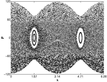
        b

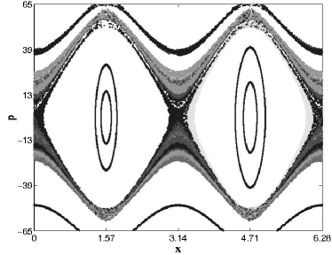
Figure 3: The same as in FIG. 2 with $s_{z}(0)=-0.863$ and $p(0)=1.$ Change of density appears after (a) $\Delta\tau=75,000$ and $\delta=1.2$ and (b) $\Delta\tau=49,000$ and $\delta=1.92$. $x,p$ are dimensionless.

a

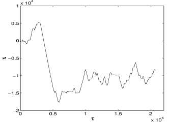
        b

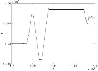
        c

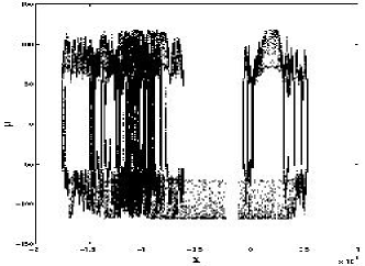
Figure 4: Lévy flights of an atom in a cavity. (a) A long ballistic flight at $\delta=1.2$ is evident. (b) Ballistic flights intermittent with stagnation phases of motion at $\delta=1.92$ are shown. (c) Two different types of the Lévy flights in the plane $x-p$. Time is in units of $\Omega_{0}^{-1}$. $x,p,\tau$ are dimensionless.

In this section a detailed analysis of the atom and photon chaotic dynamics will be considered. A sensitive control parameter is $\delta=(\omega_{f}-\omega_{a})/\Omega_{0}$, detuning of the field and atom frequencies. For the sake of convenience we specify two values of $\delta$: 1.2 and 1.92. It follows from calculating maximal Lyapunov exponents in the previous section that the smaller is $\delta$ (in the range $0.5\lesssim\mid\delta\mid\lesssim 3$), the stronger is mixing and chaos, and one can expect that the case with $\delta=1.92$ is, being chaotic (but not with the atom prepared in the upper state or close to it), more intermittent than the case $\delta=1.2$. This property of the atom-photon dynamics will be quantitatively characterized below.

The difference of a trajectory projection on the $x-p$ plane $(a_{x}=s_{x}=0$) is evident from FIG. 3 where the density modulation has been used: a change of each density appears after $\Delta\tau$ points of the mapping the trajectories ($\Delta\tau=75,000$ for (a) and $\Delta\tau=49,000$ for (b)). The narrow strips of the same density in FIG. 3b indicate a long stay of atom in the corresponding part of the $x-p$ plane with oscillations in the potential well and a small change of the amplitude of the oscillations. In contrast to this pattern, the distribution of densities in FIG. 3a is more uniform manifesting much better mixing, although some traces of the intermittency persist.

The difference between $\delta=1.2$ and $\delta=1.92$ is also evident from FIG. 4 where a dependence $x=x(\tau)$ is shown. The intermittent case ($\delta=1.92$) has very long “flights” known also as Lévy flights SZK ; Z98 . There are two types of flights in FIG. 4b. One category of flights corresponds to the almost linear dependence of $x=x(\tau)$, while the other one corresponds to the stagnation of the trajectory near some value of $x$. FIG. 4c shows the flight in the $x-p$ plane where the ballistic dynamics coexists or alternate stagnations. Both categories of flights are well understood from FIG. 2c,d: ballistic dynamics along $x$ in FIG. 2c is responsible for the linear dependence of $x=x(\tau)$, while the trajectory can stay very long near the saddle points as in FIG. 2d (the dark area near a saddle point). The case of $\delta=1.2$ in FIG. 2a,b is very different and flights of both categories are rare, if ever.

Just the presence of flights and intermittent behavior of the physical variables strong fluences the statistical properties of atoms and photons. We will use two important characteristics of the atom-photon variables: distribution of Poincaré recurrences and moments of the atom coordinate $x$. Consider a small phase volume $\Delta\Gamma$ and $P(\Delta\Gamma;\tau)$ as a probability density of a trajectory to return first time back to $\Delta\Gamma$ at time instant $\tau\in(\tau+d\tau)$ if initially started at $\Delta\Gamma$ at $\tau=0$. Then the density probability to return first time to $\Delta\Gamma$ is

$$P(\tau)=\lim_{\Delta\Gamma\rightarrow 0}\frac{1}{\Delta\Gamma}P(\Delta\Gamma;\tau)\,$$ (32)

with a normalization condition

$$\int_{0}^{\infty}P(\tau)d\tau=\lim_{\Delta\Gamma\rightarrow 0}\frac{1}{\Delta\Gamma}\int_{0}^{\infty}P(\Delta\Gamma;\tau)d\tau=1\ .$$ (33)

The probability $P(\tau)$ does not depend on the choice of $\Delta\Gamma$ and for “good” chaotic mixing decays exponentially ZEN

$$P(\tau)=(1/h)e^{-h\tau}\,$$ (34)

with the mean recurrence time

$$\tau_{\rm rec}=1/h=\int_{0}^{\infty}\tau P(\tau)d\tau\ ,$$ (35)

and $h$ as Kolmogorov-Sinai entropy.

The general situation is more complicated since an algebraic behavior

$$P(\tau)\sim 1/\tau^{\gamma}\ ,\quad\tau\rightarrow\infty\ ,$$ (36)

is possible for large $\tau$ due to intermittent chaos. For bounded Hamiltonian dynamics, $\tau_{\rm rec}<\infty$ (Kac lemma), and the condition $\gamma>2$ should exist. Nevertheless, strongly intermittent dynamics sometimes does not permit us to achieve the limit at $\tau\rightarrow\infty$ and many different intermediate asymptotics can appear. FIG. 5 shows the distribution of recurrences that is close to the exponential one as in (34) for $\delta=1.2$ and to the algebraic one as in (36) with $\gamma\gtrsim 2$ $(\tau>10^{5}$) for $\delta=1.92.$

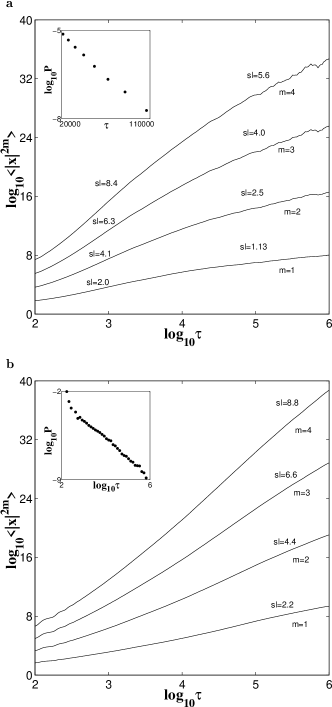
Figure 5: Time evolution of the $2m$th-order moments of the atom position $x$ on a logarithmic scale with the values of slopes indicated for each $m$. The insets show the respective distributions of the Poincaré recurrences. (a) $\delta=1.2$. (b) $\delta=1.92$. $x,\tau$ are dimensionless.

The difference due to intermittency also occurs for the moments

$$\langle x^{2m}\rangle\sim\tau^{\mu(m)}\ ,$$ (37)

where the so-called transport exponent $\mu(m)$ varies for different time windows. The behavior of $\langle x^{2m}\rangle$ is shown in FIG. 5. For $\delta=1.2$, the value $\mu(1)$ is close to 2 for $\tau<10^{3}$ and corresponds to the ballistic dynamics. For $\tau>10^{3}$ and $\delta=1.2$, we have $\mu(1)\approx 1.13$ that corresponds to a weak superdiffusion that is fairly close to the normal diffusion with $\mu(1)=1$. A very different behavior for moments appears for $\delta=1.92$ where there are many long-lasting flights. For $\tau>10^{3}$, $\mu(1)\approx 2.2$ that corresponds to a superballistic transport with an acceleration. This behavior can be explained as a result of long flights when atoms move in the photon’s field acquiring acceleration. This type of transport is self-similar and $\mu(4)\approx 8.8=4\mu(1)$.

VI Manipulation of Atoms

In this section we would like to make a few comments related to the manipulation of atoms by changing different control parameters. As it was shown in Sec. V, a change of $\delta$ leads to a possibility of a sensitive control of the Lévy flights and, as a result, to cool the atoms which have the lower chaotic dispersion the longer the flight is. At the same time, simulations show fast mixing on the $a_{x}-a_{y}$ and $s_{x}-s_{y}$ planes. More precisely, spectral properties of the atomic dynamics are sensitively controlled by the parameter $\delta$. Let us demonstrate it using a simplified analysis.

Consider $x=x(\tau)$ as the only variable that describes the dynamics or the most essential part of the dynamics, and introduce a generation function

$$G(x,\tau;\nu)=e^{i\nu[x(\tau)-x_{0}]}\ ,\ \ \ \ \ x_{0}\equiv x(0)\ .$$ (38)

Then

$$I(\tau;x_{0})\equiv\int_{-\infty}^{\infty}d\nu\ G(x,\tau;\nu)=2\pi\delta[x(\tau)-x_{0}]\ .$$ (39)

The expression $I(\tau;x_{0})$ can be “coarse-grained” over $x_{0}$, i.e.

$$\langle I(\tau;x_{0})\rangle_{x_{0}}\equiv\frac{1}{\Delta x_{0}}\int dx_{0}\,I(\tau,x_{0})=\\ =\frac{2\pi}{\Delta x_{0}}\int dx_{0}\ \delta[x(\tau)-x_{0}]\ .$$ (40)

The presence of $\delta$-function indicates recurrences to $x_{0}$ within an interval $\Delta x_{0}$ at time instant $\tau$ within an interval $\Delta\tau_{0}$. For $\tau\rightarrow\infty$ we can neglect $n$-triple recurrences from $n\geq 2$ and leave only the first recurrences. Then

$$\langle I(\tau;x_{0})\rangle_{x_{0}}=P(\tau)=\\ =\sum_{x_{0}\in\Delta x_{0}}{\rm const}/\left|\frac{dx(\tau)}{dx_{0}}\right|_{x(\tau)=x_{0}}\ .$$ (41)

The expression (41) shows that for “good” chaotic systems

$$|dx(\tau)/dx_{0}|\sim\exp(h\tau)\ ,$$ (42)

and we arrive at (34). For the intermittent dynamics, the sum in (41) consists of two types of terms, the same as (42) and the algebraic growth

$$|dx/dx_{0}|\sim\tau^{\gamma}\ ,$$ (43)

with the value of $\gamma$ depending on the type of intermittency. For a fairly large $\tau$, the term (43) survives and we arrive at the case (36).

From another side,

$$\frac{\partial^{2m}}{\partial\nu^{2m}}\langle G(x,\tau;\nu\rangle_{\nu=0}=(-1)^{m}\langle|x(\tau)-x_{0}|^{2m}\rangle\ ,$$ (44)

and we obtain the moments of $x(\tau)$. This shows that the moments and their spectral properties are coupled to the recurrences distribution through the generating function $G(x,\tau;\nu)$ which one would expect to obtain from experiments. When the moments are infinite, the expression (44) can be replaced by the following one

$$\frac{\partial^{\beta}}{\partial\nu^{\beta}}\langle G(x^{\beta},\tau;\nu^{\beta}\rangle_{\nu=0}={\rm const}\ \langle|x(\tau)-x_{0}|^{\beta}\rangle\ ,$$ (45)

with an appropriate value of $\beta$ (see more discussion in SZ97 ).

a

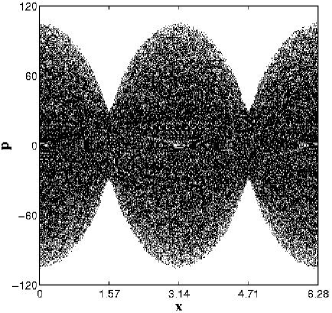
        b

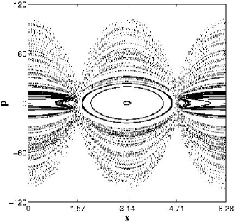
Figure 6: The same as in FIG. 2 but with $p(0)=2$, $\delta=0.4$ and the atom initially prepared nearly in its excited state with two slightly different values of the population inversion. (a) $s_{z}(0)=0.863$. (b) $s_{z}(0)=0.8660254$ (for comparison, additional trajectories with $p(0)>2$ are shown). $x,p$ are dimensionless.

The main way of controlling the properties of $G(x,\tau;\nu)$ is to change the system’s topology in phase space. Speaking about the topology, we have in mind the phase pattern (see also the end of the Sec. II) that includes the singular points, curves, and partitioning of the domains of chaos and islands. To illustrate how the system is sensitive to small variations of the initial conditions that change the full energy, we show in FIGs. 6a and b the Poincaré sections with $s_{z}(0)=0.863$ and $s_{z}(0)=0.8660254$, respectively, at $\delta=0.4$ and under the other equal conditions. Very small difference in the values of the initial tipping angle between the direction of the Bloch vector and the axis $z$ gives rise to cardinally different motion with $p(0)=2$, chaotic oscillations in the wide range of the atomic momenta with $s_{z}(0)=0.863$ and small regular translational oscillations nearly the bottom of a potential well with $s_{z}(0)=0.8660254$. Transition from order to chaos takes place with the latter value of the initial atomic population inversion only with much more large values of the initial momentum, $p(0)\gtrsim 40$.

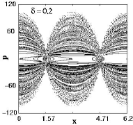
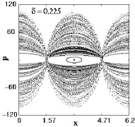
Figure 7: Bifurcation of the saddle point into the elliptic point on the plane $x-p$ under changing the detuning $\delta$. $x,p$ are dimensionless.

The original system (3) has three degrees of freedom and it is not studied yet. Nevertheless, we were able to demonstrate by simulation a bifurcation of a hyperbolic point into the elliptic one, although we are not able to provide an analytical description at the moment since the FIG. 7 is just a projection of a trajectory in the 4-dimensional hyperspace onto the plane $(p,x)$. By a change of $\delta$ near $\delta^{*}\sim 0.222$, the saddle on the $x-p$ plane with $a_{x}=s_{x}=0$ transforms into the elliptic point. The trapping potential well of the finite size on $x-p$ plane occurs as a result of the bifurcation: this bifurcation will be studied in detail in another paper.

VII Conclusion

A system with one or more cold atoms strongly coupled to a single mode of the cavity field is ideal for testing fundamentals of quantum mechanics and its corresponding to classical mechanics. Based on our understanding of the nonlinear dynamics of the atom-photon interaction in a standing-wave high-finesse cavity, new ways to manipulate and control atomic motion can be opened. We have shown that the motion is very sensitive to the atom-cavity detuning $\delta$. Varying $\delta$, one can design topology of the underlying phase space creating zones of trapping, quasi-trapping or acceleration, quasi-regular and stochastic webs, etc. It may provide new schemes for cooling, trapping, and accelerating atoms.

To give an idea about the values of the magnitudes we have used in numerical simulations, we need to estimate the range of values of the normalized recoil frequency $\alpha=\hbar k_{f}^{2}/m\Omega_{0}$ with real atoms and cavities. We will use the parameters of the real experiments with single atoms in the strong-coupling regime Y99 ; MF99 , for which the maximal atom-field coupling strength $\Omega_{0}$ exceeds the decay rates of the cavity field and of the atomic dipole. Atoms were collected in a magneto-optical trap and cooled down to microKelvin temperatures, before entering a microscopic high-finesse Fabry-Perot cavity with $Q\simeq 10^{6}$, $\Omega_{0}\simeq 2\pi(10^{7}-10^{8})$ Hz and $k_{f}\simeq 2\pi\cdot 10^{6}m^{-1}$. With these values of the parameters, one can estimate $\alpha$ to be in the range $10^{-5}-10^{-2}$ depending on the atomic mass and $\Omega_{0}$.

VIII Acknowledgment

We thank L.E. Kon’kov for his help in preparing FIG. 1. This work was supported by the Russian Foundation for Basic Research under Grant No. 02-02-17796; the Office of Naval Research, Grants No. N00014-96-1-0055 and No. N00014-97-1-0426, and U.S. Department of Energy Grant No. DE-FG02-92ER54184. The simulations were supported by the National Science Foundation cooperative agreement No. AC1-9619020 through computing resources provided by the National Partnership for Advanced Computational Infrastructure at the San Diego Supercomputer Center. S.P. thanks the Courant Institute of Mathematical Sciences, New York University, for the hospitality during his stay.

References

- (1) Cavity Quantum Electrodynamics, edited by P.R. Berman (Academic, New York, 1994).
- (2) C.S. Adams, M. Sigel, and J. Mlynek, Phys. Rep. 240, 143 (1994).
- (3) J. Ye, D.W. Vernooy, and H.J. Kimble, Phys. Rev. Lett. 83, 4987 (1999).
- (4) C.J. Hood, T.W. Lynn, A.C. Doherty, A.S. Parkins, and H.J. Kimble, Science, 287, 1447 (2000).
- (5) S.J. van Enk, J. McKeever, H.J. Kimble, and J. Ye, Phys. Rev. A 64, 013407 (2001).
- (6) P. Munstermann, T. Fischer, P. Maunz, P.W.H. Pinkse, and G. Rempe, Phys. Rev. Lett. 82, 3791 (1999).
- (7) P.W.H. Pinkse, T. Fischer, P. Maunz, and G. Rempe, Nature 404, 365 (2000).
- (8) D.J. Wineland, C. Monroe, W.M. Itano, D. Leibfried, B.E. King, and D.M. Meekhof, J. Res. Natl. Inst. Stand. Technol. 103, 259 (1998).
- (9) C. Monroe, D.M. Meekhof, B.E. King, and D.J. Wineland, Science 272, 111 (1996).
- (10) J.I. Cirac and P. Zoller, Phys. Rev. Lett. 74, 4091 (1995).
- (11) C. Monroe, D.M. Meekhof, B.E. King, W.M. Itano, and D.J. Wineland, Phys. Rev. Lett. 75, 4714 (1995).
- (12) G.M. Zaslavsky, Phys. Rep. 80, 157 (1981).
- (13) F. Haake, Quantum Signatures of Chaos (Springer, Berlin, 1991).
- (14) W.H. Zurek, Phys. Today 44, 36 (1991).
- (15) D. Giulini, E. Joos, G. Kiefer, J. Kupsch, L.-O. Stamatescu, and H.D. Zeh, Decoherence and the Appearance of a Classical World in Quantum Theory (Springer, Berlin, 1996).
- (16) H. Haken, Phys. Lett. A. 53, 77 (1975).
- (17) P.I. Belobrov, G.M. Zaslavskii, and G.Kh. Tartakovskii, Zh. Éksp. Teor. Fiz. 71, 1799 (1976) [Sov. Phys. JETP 44, 945 (1976)].
- (18) G.P. Berman, E.N. Bulgakov, and G.M. Zaslavsky, Chaos 2, 257 (1992).
- (19) G.P. Berman and G.M. Zaslavsky, Physica A 91, 450 (1978).
- (20) S.V. Prants and L.E. Kon’kov, Phys. Lett. A 225, 33 (1997).
- (21) S.V. Prants, L.E. Kon’kov, and I.L. Kirilyuk, Phys. Rev. E 60, 335 (1999).
- (22) V.I. Ioussoupov, L.E. Kon’kov, and S.V. Prants, Physica D 155, 311 (2001).
- (23) S.V. Prants, Phys. Rev. E 61, 1386 (2000).
- (24) S.V. Prants and L.E. Kon’kov, Phys. Rev. E 61, 3632 (2000).
- (25) F.L. Moore, J.C. Robinson, C. Bharucha, P.E. Williams, and M.G. Raizen, Phys. Rev. Lett. 73, 2974 (1994).
- (26) W.K. Hensinger, A.G. Truscott, B. Upcroft, M. Hug, H.M. Wiseman, N.R. Heckenberg, and H. Rubinsztein-Dunlop, Phys. Rev. A 64, 033407 (2001).
- (27) R. Graham, M. Schlautmann, and P. Zoller, Phys. Rev. A 45, R19 (1992).
- (28) F.L. Moore, J.C. Robinson, C.F. Bharucha, Bala Sundaram, and M.G. Raizen, Phys. Rev. Lett. 75, 4598 (1995).
- (29) H. Ammann, R. Gray, I. Shvarchuck, and N. Christensen, Phys. Rev. Lett. 80, 4111 (1998).
- (30) M.F. Shlesinger, G.M. Zaslavsky, and J. Klafter, Nature 363, 31 (1993).
- (31) G.M. Zaslavsky, Physics of Chaos in Hamiltonian Systems (Imperial College Press, London, 1998).
- (32) B.G. Klappauf, W.H. Oskay, D.A. Steck, and M.G. Raizen, Phys. Rev. Lett. 81, 4044 (1998).
- (33) B. Sundaram and G.M. Zaslavsky, Phys. Rev. E 59, 7231 (1999).
- (34) A. Iomin and G.M. Zaslavsky, Phys. Rev. E 60, 7580 (1999).
- (35) R. Artuso and M. Rusconi, Phys. Rev. E 64, 015204-1 (2001).
- (36) F. Bardou, J.P. Bouchaud, O. Emile, A. Aspect, and C. Cohen-Tannoudji, Phys. Rev. Lett. 72, 203 (1994).
- (37) J. Reichel, F. Bardou, M. Ben Dahan, E. Peik, S. Rand, C. Salomon, and C. Cohen-Tannoudji, Phys. Rev. Lett. 75, 4575 (1995).
- (38) B. Saubaméa, M. Leduc, and C. Cohen-Tannoudji, Phys. Rev. Lett. 83, 3796 (1999).
- (39) S.V. Prants and L.E. Kon’kov, Pis’ma Zh. Éksp. Teor. Fiz. 73, 200 (2001) [JETP Lett. 73, 180 (2001)].
- (40) S.V. Prants and V.Yu. Sirotkin, Phys. Rev. A 64, 3412 (2001).
- (41) E.T. Jaynes and F.W. Cummings, Proc. IEEE 51, 89 (1963).
- (42) G.M. Zaslavsky, R.Z. Sagdeev, D.A. Usikov, and A.A. Chernikov, Weak Chaos and Quasiregular Patterns (Cambridge University Press, Cambridge, England, 1991).
- (43) A.J. Lichtenberg and M.A. Lieberman, Regular and Stochastic Motion (Springer, New York, 1983).
- (44) G.M. Zaslavsky, M. Edelman, and B. Niyasov, Chaos 7, 159 (1997).
- (45) A.I. Saichev and G.M. Zaslavsky, Chaos 7, 753 (1997).
- (46) K.T. Alligood, T.D. Sauer, and J.A. Yorke, Chaos: an Introduction to Dynamical Systems (Springer, New York, 1997)
- (47) V.I. Arnold, Mathematical Methods in Classical Mechanics (Springer, New York, 1988)