Abstract

We determine conditions for the quantisation of graphs using the Dirac operator for both two and four component spinors. According to the Bohigas-Giannoni-Schmit conjecture for such systems with time-reversal symmetry the energy level statistics are expected, in the semiclassical limit, to correspond to those of random matrices from the Gaussian symplectic ensemble. This is confirmed by numerical investigation. The scattering matrix used to formulate the quantisation condition is found to be independent of the type of spinor. We derive an exact trace formula for the spectrum and use this to investigate the form factor in the diagonal approximation.

1 Introduction

Quantum graphs have proved an important model in the semiclassical study of systems whose classical analogues are chaotic [16, 17]. Much work in this field concerns the conjecture of Bohigas, Giannoni and Schmit [6] which connects statistics of the energy level spectrum to those of random matrices, the ensemble of random matrices depending on the symmetries of the system. For systems with no time-reversal symmetry statistics of the Gaussian unitary ensemble (GUE) are expected whereas those of the Gaussian orthogonal (GOE) or symplectic (GSE) ensemble should apply for systems with time-reversal symmetry, depending on whether the spin is integer or half integer, respectively. Most investigations of this conjecture have concentrated on systems with spin zero and there are few examples of systems whose energy level statistics follow the GSE prediction [20, 11, 19, 21, 14]. In line with this the usual graph quantisation applies the Schrödinger operator to a metric graph, finding energy level statistics of the GOE or GUE [16, 17].

It is our aim to develop a quantisation of graphs including half integer spin and we expect to observe spectral statistics following the GSE when time-reversal symmetry is present. We choose a Dirac operator that we realise as a self-adjoint operator on an appropriate Hilbert space. The Dirac operator on a graph was considered previously by Bulla and Trenkler [10] as an alternative model of a simple scattering system, however, without addressing the problem of time-reversal invariance. Instead we take closed graphs and find boundary conditions that ensure a self-adjoint realisation of the Dirac operator such that time-reversal symmetry is preserved. By looking at systems of this type we can compare the spectrum with the results for the Schrödinger operator on graphs and general semiclassical results for systems with spin. One well known advantage of the quantum graph is that the trace formula is exact rather than semiclassical. This provides the opportunity to distinguish features present only in the semiclassical limit from those inherent in systems with spin.

One unusual quality of the Dirac operator in one dimension is the possibility of two component spinors rather than the usual four component spinors required in three dimensions. Physically this appears odd. If the Dirac operator on the graph describes an idealisation of a physical system of wires in the limit that the width of the wire tends to zero we are lead to four component spinors of the type required in three dimensions. If however we set up the mathematical problem in which the graph is a topological entity then it is natural to choose two component spinors. In the context of quantising graphs the apparent contradiction will in fact disappear. The spectrum is independent of the choice of spinors so the physics of the system cannot distinguish the language used to describe it.

Our paper is organised as follows: In section 2 we introduce the necessary terminology of graphs. Section 3 sets out the two approaches to the Dirac operator in one dimension, restricting from the Dirac equation in three dimensions which leads to four component spinors or considering an irreducible representation of the Dirac algebra which requires only spinors with two components. In section 4 we find self-adjoint and time-reversal symmetric realisations of the Dirac operator for two component spinors and in section 5 we do the same in the four component case. Numerical examples confirm that even for simple graphs the energy level statistics follow the GSE prediction. We find that the scattering matrix in both formalisms has the same properties, the spectrum is therefore independent of the approach taken. In section 6 we first derive the exact trace formula for the density of states and then use this to calculate the form factor. Making the diagonal approximation we see that the form factor agrees with the GSE result for low $\tau$. Finally we suggest how the recipe for quantising a graph with the Dirac operator is consistent with the model of a graph as a three dimensional system of wires, section 7.

2 Graphs

We begin with a few general definitions necessary when considering graphs. A graph consists of $V$ vertices connected by $B$ bonds. The valency $v_{i}$ of a vertex $i$ is the number of bonds meeting at the vertex. The topology of a graph can be described using its connectivity matrix $C$. This is a $V\times V$ matrix with entries

$$C_{ij}:=\left\{\begin{array}[]{cl}1&\textrm{if vertices $i$ and $j$ are connected},\\ 0&\textrm{otherwise},\\ \end{array}\right.$$ (2.1)

where we have assumed that the graph has at most one bond connecting any pair of vertices. We also suppose the graphs under consideration to be connected, any vertex can be reached from any other by passing down bonds. A graph is directed if the bonds are assigned directions: A bond running from vertex $i$ to vertex $j$ will be denoted as $b=(ij)$.

On a graph one usually considers probabilistic rather than deterministic classical dynamics. This can be described by a stochastic matrix $M$ of transition probabilities between the bonds. The matrix $M=(M_{bc})$ defines a Markov chain on the graph propagating vectors $\rho=(\rho_{1},\dots,\rho_{2B})^{T}$ of probabilities assigned to the bonds, $\rho\mapsto M\rho$. Note that we allow particles to move in either direction on a bond and so there are $2B$ possible states of the particle on the graph. (This convention for counting bonds will prove necessary later as plane-wave solutions for the Dirac operator cannot be made to correspond to the directions on a directed graph as in the Schrödinger case.) The non-negative matrix $M$ is called irreducible if for every pair $(b,c)$ of states there exists a power $q$ such that $(M^{q})_{bc}>0$. If the power $q$ can be chosen independent of $(b,c)$, such that all elements of the matrix $M^{q}$ are strictly positive, $M$ is called primitive. A Markov chain with an irreducible Markov matrix $M$ is ergodic, i.e. any initial distribution $\rho$ converges in average to the stable distribution $\rho_{0}=\frac{1}{2B}(1,\dots,1)^{T}$,

$$\lim_{N\to\infty}\frac{1}{N}\sum_{n=1}^{N}M^{n}\rho=\rho_{0}\ .$$ (2.2)

A Markov matrix corresponding to an ergodic chain has a non-degenerate eigenvalue one. For primitive stochastic matrices all other eigenvalues are smaller in magnitude such that the associated Markov process is mixing. Then an initial distribution converges to the stable distribution,

$$\lim_{n\to\infty}M^{n}\rho=\rho_{0}\ ,$$ (2.3)

and, moreover,

$$\lim_{n\to\infty}(M^{n})_{bc}=\frac{1}{2B}\ .$$ (2.4)

It is this last condition that will be used in section 6.2 to evaluate the form factor in the diagonal approximation. Details on non-negative matrices and Markov chains can be found in [12].

If the quantum system on the graph is defined by a matrix ${\mathbb{T}}=(T_{bc})$ of complex transition amplitudes between the bonds (we will see that ${\mathbb{T}}$ is unitary) then

$$M_{(ij)(ki)}=|T_{(ij)(ki)}|^{2}\ .$$ (2.5)

$M_{(ij)(ki)}$ is the quantum mechanical probability that a particle traveling from $k$ to $i$ scatters at $i$ to travel towards the vertex $j$. The unitarity of ${\mathbb{T}}$ implies that $M$ is doubly stochastic and therefore defines a Markov chain.

While only topological information is necessary to investigate classical dynamics on a graph quantum mechanics requires us to assign lengths, $L_{(ij)}$, to bonds, $(ij)$. This defines a metric graph. It is natural to consider a bond with length as directed, one vertex lying at zero on the bond and the other at $L$, consequently our metric graphs are also directed graphs. In order to avoid degeneracies in the lengths of periodic orbits on the graph we assume the lengths assigned to the bonds are incommensurate, not related by a rational number.

3 The Dirac equation in one dimension

In one spatial dimension the Dirac equation is

$$\textrm{i}\hbar\frac{\partial}{\partial t}\Psi(x,t)=\left(-\textrm{i}\hbar c\,\alpha\,\frac{\partial}{\partial x}+mc^{2}\,\beta\,\right)\Psi(x,t)\ ,$$ (3.1)

where $\alpha$ and $\beta$ satisfy the relations $\alpha^{2}=\beta^{2}=\textrm{I}$ and $\alpha\beta+\beta\alpha=0$ that define the Dirac algebra. There are two possible interpretations of this equation: Either one views it as a restriction of the Dirac equation in three dimensions, or one considers it as a problem in one dimension from the outset. In the first case this equation originates from an implementation of the Poincaré space-time symmetries in relativistic quantum mechanics such that the notions of spin and of anti-particles can be carried over. If then, for instance, one restricts to the $y$ axis the Dirac matrices $\alpha=\alpha_{y}$ and $\beta$ are hermitian $4\times 4$ matrices that form a reducible representation of the Dirac algebra in one dimension. The second case is void of the physical interpretations deriving from $3+1$-dimensional space-time symmetries. One merely considers the Dirac equation (3.1) with a faithful irreducible representation of the Dirac algebra and thus chooses $\alpha$ and $\beta$ to be hermitian $2\times 2$ matrices. For an extensive discussion of the Dirac equation see [22].

The two cases are naturally connected as a unitary transformation of $\alpha_{y}$ and $\beta$ brings them into block diagonal form preserving the algebraic relations. For example the standard (Dirac) representation of the matrices in three dimensions, restricted to the $y$ axis, is

$$\alpha=\left(\begin{array}[]{cccc}0&0&0&-\textrm{i}\\ 0&0&\textrm{i}&0\\ 0&-\textrm{i}&0&0\\ \textrm{i}&0&0&0\\ \end{array}\right)\ ,\qquad\beta=\left(\begin{array}[]{cccc}1&0&0&0\\ 0&1&0&0\\ 0&0&-1&0\\ 0&0&0&-1\\ \end{array}\right).$$ (3.2)

Now consider the unitary transformation

$$U=\frac{1}{\sqrt{2}}\left(\begin{array}[]{cccc}1&1&0&0\\ 0&0&-1&1\\ -1&1&0&0\\ 0&0&1&1\\ \end{array}\right).$$ (3.3)

Applying $U$ to $\alpha$ and $\beta$ generates a new representation,

$$U\alpha U^{-1}=\left(\begin{array}[]{cccc}0&-\textrm{i}&0&0\\ \textrm{i}&0&0&0\\ 0&0&0&\textrm{i}\\ 0&0&-\textrm{i}&0\\ \end{array}\right)\ ,\qquad U\beta U^{-1}=\left(\begin{array}[]{cccc}1&0&0&0\\ 0&-1&0&0\\ 0&0&1&0\\ 0&0&0&-1\\ \end{array}\right)\ ,$$ (3.4)

which is obviously reducible. Either of the $2\times 2$ blocks represents the Dirac algebra in one dimension irreducibly. It is, however, important to note that passing from the four dimensional to the two dimensional representation the usual interpretations of spin, particles and anti-particles, and time-reversal are lost.

For both two- and four-dimensional representations of the Dirac algebra the Dirac operator reads

$$\mathcal{D}:=-\textrm{i}\hbar c\,\alpha\,\frac{\mathrm{d}}{\mathrm{d}x}+mc^{2}\,\beta\ .$$ (3.5)

On the real line $\mathcal{D}$ is defined as an essentially self-adjoint operator on the Hilbert space $L^{2}({\mathbb{R}})\otimes{\mathbb{C}}^{n}$ with domain $C_{0}^{\infty}({\mathbb{R}})\otimes{\mathbb{C}}^{n}$, where $n=2$ or $n=4$.

In order to obtain self-adjoint realisations of the Dirac operator on a compact interval $I=[0,L]$ appropriate boundary conditions have to be specified. These can be classified by extensions of the closed symmetric operator $\mathcal{D}^{0}$ given as $\mathcal{D}$ defined on the domain $W_{2,1}^{0}(I)\otimes{\mathbb{C}}^{n}\subset L^{2}(I)\otimes{\mathbb{C}}^{n}$. Here $W_{2,1}^{0}(I)$ denotes the Sobolev space of functions $\varphi$ on $I$ that are, along with their (generalised) first derivatives, in $L^{2}(I)$ and satisfy $\varphi(0)=0=\varphi(L)$. The closed symmetric extensions of $\mathcal{D}^{0}$ arise from restrictions of $\mathcal{D}$ defined on the domain $W_{2,1}(I)\otimes{\mathbb{C}}^{n}$ of $n$-component Sobolev spinors with no specified boundary conditions to subspaces on which the skew-Hermitian quadratic form

$$\Omega(\phi,\psi):=\langle\mathcal{D}\phi,\psi\rangle-\langle\phi,\mathcal{D}\psi\rangle$$ (3.6)

vanishes. The maximal isotropic subspaces of $W_{2,1}(I)\otimes{\mathbb{C}}^{n}$ with respect to $\Omega$, i.e. the maximal subspaces on which $\Omega$ vanishes, then yield domains on which $\mathcal{D}$ is self-adjoint. This is the approach adopted by Kostrykin and Schrader for the Schrödinger operator [15] on graphs. Self-adjoint realisations of the Dirac operator on an interval are also classified using a different technique by Alonso and De Vincenzo [1].

4 The Dirac operator for two component spinors

From the two approaches to the problem we begin with the minimum necessary and consider two component spinors first. According to the above we take

$$\alpha=\left(\begin{array}[]{cc}0&-\textrm{i}\\ \textrm{i}&0\\ \end{array}\right)\ ,\qquad\beta=\left(\begin{array}[]{cc}1&0\\ 0&-1\\ \end{array}\right).$$ (4.1)

(The choice of $\alpha$ and $\beta$ is designed to simplify the calculations.)

Eigenspinors $\psi=\binom{\psi_{1}}{\psi_{2}}$ of $\mathcal{D}$ are solutions of the time independent Dirac equation

$$\mathcal{D}\psi(x)=E\psi(x)\ .$$ (4.2)

For positive energies $E$ they are hence plane waves of the form

$$\psi_{k}(x)=\mu(k)\left(\begin{array}[]{c}1\\ \textrm{i}\gamma(k)\\ \end{array}\right)\textrm{e}^{\textrm{i}kx}+\hat{\mu}(k)\left(\begin{array}[]{c}1\\ -\textrm{i}\gamma(k)\\ \end{array}\right)\textrm{e}^{-\textrm{i}kx}$$ (4.3)

with $k>0$ and

$$\gamma(k):=\frac{E-mc^{2}}{\hbar ck}\ ,\qquad E=\sqrt{(\hbar ck)^{2}+m^{2}c^{4}}\ .$$ (4.4)

The choice of the coefficients $\mu(k)$ and $\hat{\mu}(k)$ depends on the boundary conditions imposed by the self-adjoint realisation of $\mathcal{D}$. We see immediately that the plane-wave spinor (4.3) is not invariant changing $x$ to $-x$. As the Dirac operator is first order the direction assigned to bonds on the graph becomes significant.

4.1 Self-adjoint realisations on graphs

Self-adjoint realisations of the Dirac operator on graphs were considered by Bulla and Trenkler [10]. However, in order to develop a simple form related to the vertex transition matrix, we continue with the approach of Kostrykin and Schrader [15] for the Schrödinger operator.

The basic idea is to view a graph as a collection of intervals that are glued together according to the connectivity matrix $C$. The Hilbert space on which the Dirac operator acts is therefore the direct sum of the Hilbert spaces for each bond,

$${\mathcal{H}}:=\bigoplus_{b=1}^{B}L^{2}\bigl{(}[0,L_{b}]\bigr{)}\otimes{\mathbb{C}}^{2}\ ,$$ (4.5)

where $b$ runs over all bonds. The spinors $\psi\in{\mathcal{H}}$ therefore consist of the $B$ components $(\psi^{1},\dots,\psi^{B})$ attached to the bonds, each of which is a two-spinor. The scalar product of spinors on the graph is then

$$\langle\phi,\psi\rangle=\sum_{b=1}^{B}\langle\phi^{b},\psi^{b}\rangle_{b}\ ,$$ (4.6)

where $\langle\phi^{b},\psi^{b}\rangle_{b}$ is the scalar product in $L^{2}\bigl{(}[0,L_{b}]\bigr{)}\otimes{\mathbb{C}}^{2}$. Self-adjoint realisations of $\mathcal{D}$ are constructed in analogy to the case of a single interval by suitably extending the closed symmetric operator $\mathcal{D}^{0}$ defined on the domain

$$\bigoplus_{b=1}^{B}W^{0}_{2,1}\bigl{(}[0,L_{b}]\bigr{)}\otimes{\mathbb{C}}^{2}\ .$$ (4.7)

The domains of its closed symmetric extensions are the isotropic subspaces of

$$\bigoplus_{b=1}^{B}W_{2,1}\bigl{(}[0,L_{b}]\bigr{)}\otimes{\mathbb{C}}^{2}$$ (4.8)

with respect to the skew-Hermitian form $\Omega$ as given in (3.6). Integrating by parts yields

$$\Omega(\phi,\psi)=\hbar c\sum_{b=1}^{B}\Bigl{(}\psi^{b}_{1}(0)\overline{\phi}^{b}_{2}(0)-\psi^{b}_{1}(L_{b})\overline{\phi}_{2}^{b}(L_{b})-\psi^{b}_{2}(0)\overline{\phi}_{1}^{b}(0)+\psi^{b}_{2}(L_{b})\overline{\phi}_{1}^{b}(L_{b})\Bigl{)}\ ,$$ (4.9)

showing that $\Omega$ only depends on the boundary values of the spinor components. Self-adjoint extensions again correspond to maximally isotropic subspaces and thus can be characterised by boundary conditions.

Following the construction of Kostrykin and Schrader [15] for Schrödinger operators on graphs, we introduce a map from the infinite-dimensional Hilbert space ${\mathcal{H}}$ to the $4B$-dimensional space of boundary values, $\psi\mapsto\boldsymbol{\psi}=\left(\begin{smallmatrix}\boldsymbol{\psi}_{1}\\ \boldsymbol{\psi}_{2}\end{smallmatrix}\right)$, with

$$\begin{split}\boldsymbol{\psi}_{1}&:=\bigl{(}\psi_{1}^{1}(0),\dots,\psi_{1}^{B}(0),\psi_{1}^{1}(L_{1}),\dots,\psi_{1}^{B}(L_{B})\bigr{)}^{T}\ ,\\ \boldsymbol{\psi}_{2}&:=\bigl{(}-\psi_{2}^{1}(0),\dots,-\psi_{2}^{B}(0),\psi_{2}^{1}(L_{1}),\dots,\psi_{2}^{B}(L_{B})\bigr{)}^{T}\ .\end{split}$$ (4.10)

By including $\psi_{2}(0)$ with a minus sign we can write $\Omega$ as

$$\Omega(\phi,\psi)=(\begin{array}[]{cc}\boldsymbol{\phi}_{1}^{\dagger}&\boldsymbol{\phi}_{2}^{\dagger}\\ \end{array})\left(\begin{array}[]{cc}0&\textrm{I}_{2B}\\ -\textrm{I}_{2B}&0\\ \end{array}\right)\left(\begin{array}[]{c}\boldsymbol{\psi}_{1}\\ \boldsymbol{\psi}_{2}\\ \end{array}\right)\ .$$ (4.11)

The maximal isotropic subspaces in (4.8) with respect to $\Omega$ are now equivalent to maximal subspaces of vectors $\boldsymbol{\psi}\in\mathbb{C}^{4B}$ on which the complex symplectic form (4.11) vanishes. Defining a linear subspace of $\mathbb{C}^{4B}$ as the vectors $\boldsymbol{\psi}$ satisfying

$${\mathbb{A}}\boldsymbol{\psi}_{1}+{\mathbb{B}}\boldsymbol{\psi}_{2}=0\ ,$$ (4.12)

with complex $2B\times 2B$ matrices ${\mathbb{A}}$ and ${\mathbb{B}}$, one first observes that in order for this subspace to have the desired dimension $2B$ the $2B\times 4B$ matrix $({\mathbb{A}},{\mathbb{B}})$ must have maximal rank. Kostrykin and Schrader show that such a subspace is maximally isotropic if and only if $({\mathbb{A}},{\mathbb{B}})$ has maximal rank and ${\mathbb{A}}{\mathbb{B}}^{\dagger}$ is hermitian.

Equation (4.12) defines boundary conditions for the Dirac operator on a collection of $B$ bonds. These boundary conditions yield a self-adjoint realisation of ${\mathcal{D}}$ when

$$\operatorname{rank}({\mathbb{A}},{\mathbb{B}})=2B\quad\text{and}\quad{\mathbb{A}}{\mathbb{B}}^{\dagger}={\mathbb{B}}{\mathbb{A}}^{\dagger}\ .$$ (4.13)

So far the connectivity of the graph has played no role. In order to implement this we consider only boundary conditions, specified through the matrices ${\mathbb{A}}$ and ${\mathbb{B}}$, that connect bonds according to the connectivity matrix $C$. The matrices ${\mathbb{A}}$ and ${\mathbb{B}}$ then have a block structure, each block defining boundary conditions at a single vertex.

Figure 1: An isolated vertex on which we wish to define the transition matrix.

At a given vertex $i$ we label the $v_{i}$ bonds such that the first $w_{i}$ bonds are outgoing and the remainder incoming, see figure 1. The vector $\boldsymbol{\psi}^{(i)}=\left(\begin{smallmatrix}\boldsymbol{\psi}_{1}^{(i)}\\ \boldsymbol{\psi}_{2}^{(i)}\end{smallmatrix}\right)\in{\mathbb{C}}^{2v_{i}}$ of boundary values at $i$ then consists of the components

$$\begin{split}\boldsymbol{\psi}_{1}^{(i)}&=\bigl{(}\psi_{1}^{1}(0),\dots,\psi_{1}^{w_{i}}(0),\psi_{1}^{w_{i}+1}(L_{w_{i}+1}),\dots,\psi_{1}^{v_{i}}(L_{v_{i}})\bigr{)}^{T}\ ,\\ \boldsymbol{\psi}_{2}^{(i)}&=\bigl{(}-\psi_{2}^{1}(0),\dots,-\psi_{2}^{w_{i}}(0),\psi_{2}^{w_{i}+1}(L_{w_{i}+1}),\dots,\psi_{2}^{v_{i}}(L_{v_{i}})\bigr{)}^{T}\ .\end{split}$$ (4.14)

If we denote the $v_{i}\times v_{i}$ blocks of the matrices ${\mathbb{A}}$ and ${\mathbb{B}}$ that define the boundary conditions at $i$ by ${\mathbb{A}}^{(i)}$ and ${\mathbb{B}}^{(i)}$, we have the condition

$${\mathbb{A}}^{(i)}\boldsymbol{\psi}_{1}^{(i)}+{\mathbb{B}}^{(i)}\boldsymbol{\psi}_{2}^{(i)}=0\quad\textrm{ with }\quad{\mathbb{A}}^{(i)}{\mathbb{B}}^{(i)\dagger}={\mathbb{B}}^{(i)}{\mathbb{A}}^{(i)\dagger}$$ (4.15)

which guarantees current conservation at the vertex $i$.

Eigenspinors $\psi$ of the Dirac operator ${\mathcal{D}}$ with given boundary conditions are composed of plane waves, equation (4.3), on each of the bonds. Assigning incoming and outgoing plane-wave solutions to each of the bonds we can write down vectors of coefficients $\boldsymbol{\overrightarrow{\mu}}$, $\boldsymbol{\overleftarrow{\mu}}$ for the outgoing and incoming waves at the vertex, respectively:

$$\boldsymbol{\overrightarrow{\mu}}=\left(\begin{array}[]{c}\mu^{1}\\ \vdots\\ \mu^{w_{i}}\\ \hat{\mu}^{w_{i}+1}\,\textrm{e}^{-\textrm{i}kL_{w_{i}+1}}\\ \vdots\\ \hat{\mu}^{v_{i}}\,\textrm{e}^{-\textrm{i}kL_{v_{i}}}\end{array}\right)\ ,\qquad\boldsymbol{\overleftarrow{\mu}}=\left(\begin{array}[]{c}\hat{\mu}^{1}\\ \vdots\\ \hat{\mu}^{w_{i}}\\ \mu^{w_{i}+1}\,\textrm{e}^{\textrm{i}kL_{w_{i}+1}}\\ \vdots\\ \mu^{v_{i}}\,\textrm{e}^{\textrm{i}kL_{v_{i}}}\\ \end{array}\right)\ .$$ (4.16)

Here we omit the index $i$ labeling the vertex. Writing $\boldsymbol{\psi}_{1}^{(i)}$ and $\boldsymbol{\psi}_{2}^{(i)}$ in terms of $\boldsymbol{\overrightarrow{\mu}}$ and $\boldsymbol{\overleftarrow{\mu}}$ and substituting into the definition of the boundary conditions we obtain

$$\boldsymbol{\overrightarrow{\mu}}=-({\mathbb{A}}^{(i)}+\textrm{i}\gamma(k){\mathbb{B}}^{(i)})^{-1}({\mathbb{A}}^{(i)}-\textrm{i}\gamma(k){\mathbb{B}}^{(i)})\,\boldsymbol{\overleftarrow{\mu}}\ .$$ (4.17)

Notice that under the conditions given the matrices $({\mathbb{A}}^{(i)}\pm\textrm{i}\gamma(k){\mathbb{B}}^{(i)})$ are always invertible [15]. This defines the vertex transition matrix ${\mathbb{T}}^{(i)}$ which connects the coefficients of incoming and outgoing plane waves at the vertex $i$,

$${\mathbb{T}}^{(i)}:=-({\mathbb{A}}^{(i)}+\textrm{i}\gamma(k){\mathbb{B}}^{(i)})^{-1}({\mathbb{A}}^{(i)}-\textrm{i}\gamma(k){\mathbb{B}}^{(i)})\ .$$ (4.18)

The condition that ${\mathbb{A}}^{(i)}{\mathbb{B}}^{(i)\dagger}$ is hermitian implies that the matrix ${\mathbb{T}}^{(i)}$ is unitary,

$$({\mathbb{T}}^{(i)})^{-1}=({\mathbb{T}}^{(i)})^{{\dagger}}\ .$$ (4.19)

Self-adjoint realisations of the Dirac operator on the graph are defined by matrices ${\mathbb{A}},{\mathbb{B}}$ with ${\mathbb{A}}{\mathbb{B}}^{\dagger}$ hermitian. These prescribe the boundary conditions (4.12) and determine unitary vertex transition matrices (4.18) for plane waves on the graph.

4.2 Time-reversal symmetry

Following the conjecture of Bohigas, Giannoni and Schmit, we expect to find energy level statistics corresponding to those of the Gaussian symplectic ensemble (GSE) for quantum systems with half-integer spin $s$ and time-reversal symmetry. This is due to the fact that the time-reversal operator is anti-unitary and squares to $(-1)^{2s}$, imprinting a symplectic symmetry on the Hamiltonian. In the case of a two component Dirac equation in one dimension the usual interpretations of spin and time-reversal inherited from three dimensions are lost. Nevertheless, one can introduce an anti-unitary operator squaring to $-1$ that is formally identical to the time-reversal operator for two component (Pauli-) spinors in three dimensions,

$$\mathcal{T}:=\left(\begin{array}[]{cc}0&1\\ -1&0\\ \end{array}\right)\mathcal{K}\ ,$$ (4.20)

where $\mathcal{K}$ is complex conjugation. This can be interpreted as a physical time-reversal in the sense that it changes the sign of time and momentum. The matrix part of $\mathcal{T}$ is only required in order that $\mathcal{T}^{2}=-\textrm{I}$ as there is no spin operator for two component spinors. In the subsequent work we will therefore refer to (4.20) as a time-reversal operator. A full discussion of time-reversal symmetry with spin is found in the second chapter of [13].

We now determine conditions under which the vertex transition matrix is time-reversal symmetric. This will raise questions about when general time-reversal symmetric boundary conditions exist for a Dirac operator on a graph. For the system to be time-reversal symmetric $\mathcal{T}$ must commute with the Hamiltonian $\mathcal{D}$. This forces the mass term in $\mathcal{D}$ to vanish. From now on we consider only the case $m=0$ for which $\gamma(k)=1$ and time-reversal symmetry is possible with two component spinors.

Applying $\mathcal{T}$ to the plane-wave solutions on a bond (4.3) we find

$$\mathcal{T}\psi_{k}(x)=-\textrm{i}\,\overline{\mu}\left(\begin{array}[]{c}1\\ -\textrm{i}\\ \end{array}\right)\textrm{e}^{-\textrm{i}kx}+\textrm{i}\,\overline{\hat{\mu}}\left(\begin{array}[]{c}1\\ \textrm{i}\\ \end{array}\right)\textrm{e}^{\textrm{i}kx}\ .$$ (4.21)

Time-reversing spinors on all the bonds meeting at the vertex $i$ defines new vectors of outgoing and incoming waves $\boldsymbol{\overrightarrow{\mu}}_{\mathcal{T}},\boldsymbol{\overleftarrow{\mu}}_{\mathcal{T}}$,

$$\boldsymbol{\overrightarrow{\mu}}_{\mathcal{T}}=\textrm{i}\left(\begin{array}[]{cc}\textrm{I}_{w_{i}}&0\\ 0&-\textrm{I}_{(v_{i}-w_{i})}\\ \end{array}\right)\overline{(\boldsymbol{\overleftarrow{\mu}})}\ ,\qquad\boldsymbol{\overleftarrow{\mu}}_{\mathcal{T}}=\textrm{i}\left(\begin{array}[]{cc}-\textrm{I}_{w_{i}}&0\\ 0&\textrm{I}_{(v_{i}-w_{i})}\\ \end{array}\right)\overline{(\boldsymbol{\overrightarrow{\mu}})}\ .$$ (4.22)

For the vertex transition matrix to be time-reversal invariant we require

$$\boldsymbol{\overrightarrow{\mu}}_{\mathcal{T}}={\mathbb{T}}^{(i)}\,\boldsymbol{\overleftarrow{\mu}}_{\mathcal{T}}\ .$$ (4.23)

Using the definition of the vertex transition matrix, $\boldsymbol{\overrightarrow{\mu}}={\mathbb{T}}^{(i)}\boldsymbol{\overleftarrow{\mu}}$ for ${\mathbb{T}}^{(i)}$ unitary, equation (4.23) implies

$$({\mathbb{T}}^{(i)})^{T}=\left(\begin{array}[]{cc}\textrm{I}_{w_{i}}&0\\ 0&-\textrm{I}_{(v_{i}-w_{i})}\\ \end{array}\right){\mathbb{T}}^{(i)}\left(\begin{array}[]{cc}-\textrm{I}_{w_{i}}&0\\ 0&\textrm{I}_{(v_{i}-w_{i})}\\ \end{array}\right)\ .$$ (4.24)

Equation (4.24) is the condition that all vertex transition matrices must satisfy in order that the system possesses time-reversal symmetry.

Splitting ${\mathbb{T}}^{(i)}$ into four blocks equation (4.24) is equivalent to

$${\mathbb{T}}^{(i)}=\left(\begin{array}[]{cc}{\mathbb{T}}_{1}&{\mathbb{T}}_{2}\\ {\mathbb{T}}_{3}&{\mathbb{T}}_{4}\\ \end{array}\right)=\left(\begin{array}[]{cc}-{\mathbb{T}}^{T}_{1}&{\mathbb{T}}^{T}_{3}\\ {\mathbb{T}}^{T}_{2}&-{\mathbb{T}}^{T}_{4}\\ \end{array}\right)\ .$$ (4.25)

The components $T_{bc}$ of the transition matrix ${\mathbb{T}}^{(i)}$ are thus either symmetric or antisymmetric according to the alignment of the bonds at the vertex, in the sense that:

$T_{bc}=T_{cb}$
$T_{bc}=-T_{cb}$			or

This raises a number of problems. Back scattering is not possible in this scheme as $T_{bb}$ is identically zero (returning to the same bond always requires antisymmetry). Consequently it is not possible to quantise graphs containing vertices with valency one. It is also clear that the components of ${\mathbb{T}}^{(i)}$ cannot be invariant under a permutation of the bonds. But it is this natural physical property imposed by Kottos and Smilansky [16, 17] that allows them to derive a simple form of the trace formula for the Schrödinger operator on a graph. In fact we may ask if any graphs exist for which the vertex transition matrices are both unitary and satisfy the time reversal condition (4.24). There are no examples of ${\mathbb{T}}^{(i)}$ for vertices with valency one and only a trivial solution for one incoming and one outgoing bond, $v_{i}=2$. With $v_{i}=3$ there are again no solutions. The simplest nontrivial example of a transition matrix is for a vertex with valency four. In this case, with two incoming and two outgoing bonds, one possible choice of a time-reversal invariant transition matrix is

$${\mathbb{T}}^{(i)}=\frac{1}{\sqrt{2}}\left(\begin{array}[]{cccc}0&1&1&0\\ -1&0&0&1\\ 1&0&0&1\\ 0&1&-1&0\\ \end{array}\right)\ .$$ (4.26)

Clearly this is both a unitary matrix and has the symmetry and antisymmetry properties prescribed by (4.25). Physically this would represent strange boundary conditions as a spinor reaching the vertex would be prevented not only from back scattering but also from scattering down another of the bonds. However it is still reasonable to ask how closely the spectrum of a graph quantised with such a vertex transition matrix will follow the GSE prediction. In the following subsection we investigate one example of a binary graph (i.e. where all vertices have two incoming and two outgoing bonds).

4.3 Bond scattering matrix

To find the energy levels we must first determine the bond scattering matrix ${\mathbb{S}}$ for the whole graph from the transition matrices at the vertices. Let us define $\mu^{(ij)}$ to be the coefficient of the plane wave on the bond $(ij)$ traveling in the direction $i\rightarrow j$. Then $\mu^{(ji)}$ is $\hat{\mu}^{(ij)}$ in our previous notation. The bond scattering matrix ${\mathbb{S}}=(S_{(ij)(lm)})$ is defined by

$$S_{(ij)(lm)}(k)=\delta_{mi}\ T^{(m)}_{(ij)(lm)}\ \textrm{e}^{\textrm{i}kL_{(lm)}}\ .$$ (4.27)

To scatter from the spinor with coefficient $\mu^{(lm)}$ to that with $\mu^{(ij)}$ the bonds $(lm)$ and $(ij)$ must be connected at $m$. The transition amplitude is then defined by the transition matrix ${\mathbb{T}}^{(m)}$ at $m$. Before the transition the spinor collects a phase propagating along $(lm)$. Equation (4.27) is equivalent to the description of the scattering matrix as a product ${\mathbb{S}}(k)={\mathbb{T}}\,{\mathbb{D}}(k)$ where ${\mathbb{D}}(k)$ is a diagonal matrix of phases and ${\mathbb{T}}$ is a matrix of transition amplitudes for the whole graph. As there are two coefficients for the spinors on each bond ${\mathbb{S}}$ is a $2B\times 2B$ matrix. The unitarity of the vertex transition matrices and the diagonal matrix of phases ${\mathbb{D}}(k)$ ensures that ${\mathbb{S}}(k)$ is also unitary. Note that the vertex transition matrices ${\mathbb{T}}^{(m)}$ and hence the bond S-matrix still depend on the directions assigned to the bonds.

The bond S-matrix ${\mathbb{S}}(k)$ acts on the vector of coefficients $\boldsymbol{\mu}$, which is composed of the coefficients $\boldsymbol{\overrightarrow{\mu}}$ and $\boldsymbol{\overleftarrow{\mu}}$ at every vertex and therefore defines the plane wave on the graph. Energy eigenfunctions correspond to vectors $\boldsymbol{\mu}$ where

$${\mathbb{S}}(k)\boldsymbol{\mu}=\boldsymbol{\mu}\ .$$ (4.28)

The energy eigenvalues then correspond to the values of $k$ for which

$$\bigl{|}\textrm{I}_{2B}-{\mathbb{S}}(k)\bigr{|}=0\ .$$ (4.29)

This quantisation condition for the graph is the same as that for the Schrödinger operator, see [16, 17].

Figure 2: The integrated nearest neighbour spacing distribution (left) and a histogram of the spacing distribution (right) for a fully connected Dirac pentagon, with 35753 levels.

Figure 2 shows the nearest neighbour level spacing statistics for a fully connected pentagon calculated using the vertex transition matrices (4.26). Directions were assigned to the bonds to produce two incoming and two outgoing bonds at each vertex. The assignment of ${\mathbb{T}}^{(i)}$ to the vertices is still not unique as the elements of ${\mathbb{T}}^{(i)}$ also vary between bonds with the same direction. The numerics confirm that, even for this small graph with unusual boundary conditions, the energy level statistics correspond well to those of random matrices from the GSE. We now turn to consider how the quantisation of more general graphs can be realised using two component spinors and whether there exists a trace formula for the Dirac operator.

4.4 Paired bonds

We expect it should be possible to put a Dirac operator on any (topological) graph while preserving time-reversal symmetry; and the assignment of elements in the transition matrix should follow a general scheme independent of the particular bonds to which they correspond. We saw that difficulties arise due to the fact that, as opposed to the case of a Schrödinger operator, the Dirac operator is a first order differential operator, thus breaking the invariance under $x\mapsto-x$. In this section we show that a quantisation in terms of a Dirac operator can be achieved for two component spinors by replacing each bond of the classical (topological) graph with a pair of metric bonds one running in each direction.

Figure 3: An isolated vertex with paired bonds.

We maintain the realisation of a two component Dirac operator as described above, however with the constraint that each vertex $i$ has valency $2v_{i}$ with pairs of directed bonds meeting at $i$ as indicated in figure 3. The bonds in a pair replace a single bond of the given topological graph and hence are assigned the same length but run in opposite directions. This restores the physical symmetry of the problem as all the original bonds are treated equivalently. Putting plane-wave solutions, equation (4.3), on the bonds we can write an eigenfunction on a pair $b$ of bonds as

$$\begin{split}\psi_{k}^{b}(x_{b})&=\mu_{\alpha}^{b}\left(\begin{array}[]{c}1\\ \textrm{i}\\ \end{array}\right)\textrm{e}^{\textrm{i}kx_{b}}+\mu_{\beta}^{b}\left(\begin{array}[]{c}1\\ -\textrm{i}\\ \end{array}\right)\textrm{e}^{\textrm{i}kx_{b}}\\ &\quad+\hat{\mu}_{\alpha}^{b}\left(\begin{array}[]{c}1\\ \textrm{i}\\ \end{array}\right)\textrm{e}^{-\textrm{i}kx_{b}}+\hat{\mu}_{\beta}^{b}\left(\begin{array}[]{c}1\\ -\textrm{i}\\ \end{array}\right)\textrm{e}^{-\textrm{i}kx_{b}}\ ,\end{split}$$ (4.30)

where $x_{v_{i}+b}$ has been replaced by $L_{b}-x_{b}$ and the extra phases absorbed into the coefficients. The coefficients have been labeled $\alpha$ or $\beta$ according to the type of spinor, characterised by a lower component i or $-\textrm{i}$, rather than the bond on which the spinor travels. Now let us rearrange the coefficients in the vectors $\boldsymbol{\overrightarrow{\mu}}$ and $\boldsymbol{\overleftarrow{\mu}}$ so that $\alpha$ coefficients are always listed first,

$$\boldsymbol{\overrightarrow{\mu}}=\left(\begin{array}[]{c}\mu_{\alpha}^{1}\\ \mu_{\beta}^{1}\\ \vdots\\ \end{array}\right)\ ,\qquad\boldsymbol{\overleftarrow{\mu}}=\left(\begin{array}[]{c}\hat{\mu}_{\alpha}^{1}\\ \hat{\mu}_{\beta}^{1}\\ \vdots\\ \end{array}\right)\ .$$ (4.31)

The self-adjoint boundary conditions still define a unitary vertex transition matrix,

$$\boldsymbol{\overrightarrow{\mu}}={\mathbb{T}}^{(i)}\,\boldsymbol{\overleftarrow{\mu}}\quad\textrm{and}\quad({\mathbb{T}}^{(i)})^{-1}=({\mathbb{T}}^{(i)})^{\dagger}\ .$$ (4.32)

Applying the time-reversal operator (4.20) to the wavefunctions (4.30) we find time-reversed vectors $\boldsymbol{\overrightarrow{\mu}}_{\mathcal{T}},\boldsymbol{\overleftarrow{\mu}}_{\mathcal{T}}$,

$$\boldsymbol{\overrightarrow{\mu}}_{\mathcal{T}}=\textrm{i}\left(\begin{array}[]{c}\overline{\hat{\mu}_{\beta}^{1}}\\ -\overline{\hat{\mu}_{\alpha}^{1}}\\ \vdots\\ \end{array}\right)\ ,\qquad\boldsymbol{\overleftarrow{\mu}}_{\mathcal{T}}=\textrm{i}\left(\begin{array}[]{c}\overline{\mu_{\beta}^{1}}\\ -\overline{\mu_{\alpha}^{1}}\\ \vdots\\ \end{array}\right)\ .$$ (4.33)

Time-reversal invariance again implies

$$\boldsymbol{\overrightarrow{\mu}}_{\mathcal{T}}={\mathbb{T}}^{(i)}\,\boldsymbol{\overleftarrow{\mu}}_{\mathcal{T}}.$$ (4.34)

Using the definition of the transition matrix (4.32) we obtain the following condition for time-reversal invariance,

$$({\mathbb{T}}^{(i)})^{T}=\left(\begin{array}[]{ccc}J^{-1}&&\\ &\ddots&\\ &&J^{-1}\\ \end{array}\right){\mathbb{T}}^{(i)}\left(\begin{array}[]{ccc}J&&\\ &\ddots&\\ &&J\\ \end{array}\right)\ ,$$ (4.35)

where

$$J:=\left(\begin{array}[]{cc}0&1\\ -1&0\\ \end{array}\right)\ .$$ (4.36)

The form of equation (4.35) is similar to, but not the same as, the definition of a symplectic matrix.

The vertex transition matrix ${\mathbb{T}}^{(i)}$ can be divided into $2\times 2$ blocks $({\mathbb{T}}^{(i)})^{bc}$ which relate incoming spinors on the pair of bonds $b$ to outgoing spinors on the bond pair $c$. Let

$$({\mathbb{T}}^{(i)})^{bc}=\left(\begin{array}[]{cc}r&s\\ v&w\\ \end{array}\right)\ ,$$ (4.37)

then time-reversal symmetry implies

$$({\mathbb{T}}^{(i)})^{cb}=\left(\begin{array}[]{cc}w&-s\\ -v&r\\ \end{array}\right)\ ,$$ (4.38)

or equivalently,

$$({\mathbb{T}}^{(i)})^{cb}=\bigl{|}({\mathbb{T}}^{(i)})^{bc}\bigr{|}\,\left(({\mathbb{T}}^{(i)})^{bc}\right)^{-1}\ .$$ (4.39)

This suggests both a method of constructing time-reversal symmetric transition matrices and the form of permutation invariance among the bond pairs to be required. Matrices of this form can be written

$${\mathbb{T}}^{(i)}=\left(\begin{array}[]{ccc}u_{1}&&\\ &\ddots&\\ &&u_{v_{i}}\\ \end{array}\right)\left\{X\otimes\left(\begin{array}[]{cc}1&0\\ 0&1\\ \end{array}\right)\right\}\left(\begin{array}[]{ccc}u_{1}^{-1}&&\\ &\ddots&\\ &&u_{v_{i}}^{-1}\\ \end{array}\right)\ ,$$ (4.40)

where $X=(x_{bc})$ is a symmetric unitary matrix of dimension $v_{i}$ and $u_{j}\in{\mathrm{SU(2)}}$. $|x_{bc}|^{2}$ is the probability that any incoming state on the classical bond $c$ scatters to any outgoing state on the classical bond $b$. We may now choose to implement a physical permutation symmetry between the bonds of the classical graph by requiring the matrix $X$ to be invariant under permutations $\sigma$,

$$X=\sigma X\sigma^{-1}\ .$$ (4.41)

Together with the condition that $X$ is unitary this implies

$$X=\textrm{e}^{\textrm{i}\theta}\left(\begin{array}[]{ccc}q-1&&q\\ &\ddots&\\ q&&q-1\\ \end{array}\right)\quad\text{with}\quad q:=\frac{1+\textrm{e}^{\textrm{i}\omega}}{v_{i}}\ .$$ (4.42)

Unsurprisingly this is similar to the vertex transition matrix for a Schrödinger operator [16, 17] which is also symmetric unitary and permutation invariant. Here the coefficient $\omega$, which we can think of parameterising the boundary conditions, is independent of $k$. The extra phase $\textrm{e}^{\textrm{i}\theta}$ is not interesting as it corresponds only to an extra $k$ independent phase factor. Adjusting the parameter $\omega$ we see that the Dirac equation also allows both Neumann like ($\omega=0$) and Dirichlet like ($\omega=\pi$) boundary conditions. An element $u_{b}u^{-1}_{c}$ of ${\mathrm{SU(2)}}$ defines a ‘spinor rotation’ from the pair of linearly independent two component spinors incoming on bond $c$ to the outgoing pair on bond $b$.

Equations (4.40) and (4.42) define general time-reversal invariant vertex transition matrices for two component spinors. The transition amplitudes have a form of permutation invariance (4.41) and in section 6.1 we see that this allows a simple form for the trace formula to be derived. With the vertex transition matrix the bond scattering matrix for the whole graph can be defined as in equation (4.27) with unpaired bonds. The quantisation condition (4.29) is also unchanged, apart from the fact that due to doubling of the number of bonds ${\mathbb{S}}(k)$ now is a $4B\times 4B$ matrix.

5 The Dirac operator for four component spinors

Before looking at examples for the two component spinors on paired bonds we will compare with the alternative construction of the Dirac operator acting on four component spinors. Therefore, we now consider again directed graphs with $B$ unpaired bonds. In this case the time independent Dirac equation reads

$$-\textrm{i}\hbar c\,\alpha\,\frac{\mathrm{d}\psi}{\mathrm{d}x}+mc^{2}\,\beta\,\psi=E\psi\ ,$$ (5.1)

where we choose $\alpha$ and $\beta$ as in (3.2),

$$\alpha=\left(\begin{array}[]{cccc}0&0&0&-\textrm{i}\\ 0&0&\textrm{i}&0\\ 0&-\textrm{i}&0&0\\ \textrm{i}&0&0&0\\ \end{array}\right)\ ,\qquad\beta=\left(\begin{array}[]{cccc}1&0&0&0\\ 0&1&0&0\\ 0&0&-1&0\\ 0&0&0&-1\\ \end{array}\right)\ .$$ (5.2)

We could alternatively have chosen either of the other $\alpha$ matrices of the standard representation for the Dirac operator in three dimensions or used another representation entirely. The choice here simplifies the working.

Eigenspinors of ${\mathcal{D}}$ are again plane waves. For positive energy they are of the form

$$\begin{split}\psi_{k}^{b}(x_{b})&=\mu_{\alpha}^{b}\left(\begin{array}[]{c}1\\ 0\\ 0\\ \textrm{i}\gamma(k)\\ \end{array}\right)\textrm{e}^{\textrm{i}kx_{b}}+\mu_{\beta}^{b}\left(\begin{array}[]{c}0\\ 1\\ -\textrm{i}\gamma(k)\\ 0\\ \end{array}\right)\textrm{e}^{\textrm{i}kx_{b}}\\ &\quad+\hat{\mu}_{\alpha}^{b}\left(\begin{array}[]{c}1\\ 0\\ 0\\ -\textrm{i}\gamma(k)\\ \end{array}\right)\textrm{e}^{-\textrm{i}kx_{b}}+\hat{\mu}_{\beta}^{b}\left(\begin{array}[]{c}0\\ 1\\ \textrm{i}\gamma(k)\\ 0\\ \end{array}\right)\textrm{e}^{-\textrm{i}kx_{b}}\ ,\end{split}$$ (5.3)

with $k>0$. The dispersion relation and $\gamma(k)$ are as in (4.4). These four plane-wave solutions differ from the two component case although they are labeled with coefficients $\mu^{b}_{\alpha}$ etc. in analogy with the two component solutions on pairs of bonds. The wavefunction $\psi^{b}(x_{b})$ is a function on a single directed bond of a metric graph. We notice that, in contrast to the pairs of two component wavefunctions (4.30), $\psi^{b}(x_{b})$ is not invariant under a change in the bond direction $x_{b}\mapsto-x_{b}$.

5.1 Self-adjoint realisations on graphs

The construction of self-adjoint realisations of the Dirac operator on the graph proceeds in complete analogy to the case of two component spinors. We therefore must look for maximal closed subspaces of

$$\bigoplus_{b=1}^{B}W_{2,1}\bigl{(}[0,L_{b}]\bigr{)}\otimes{\mathbb{C}}^{4}$$ (5.4)

on which the skew-hermitian form

$$\Omega(\phi,\psi)=\langle\mathcal{D}\phi,\psi\rangle-\langle\phi,\mathcal{D}\psi\rangle$$ (5.5)

vanishes. In order to convert the problem to the boundary values of the spinors we integrate by parts and express $\Omega$ as a complex symplectic form,

$$\Omega(\phi,\psi)=(\begin{array}[]{cc}(\boldsymbol{\phi}^{+})^{\dagger}&(\boldsymbol{\phi}^{-})^{\dagger}\\ \end{array})\left(\begin{array}[]{cc}0&\textrm{I}_{4B}\\ -\textrm{I}_{4B}&0\\ \end{array}\right)\left(\begin{array}[]{c}\boldsymbol{\psi}^{+}\\ \boldsymbol{\psi}^{-}\\ \end{array}\right)\ ,$$ (5.6)

on ${\mathbb{C}}^{8B}$. Here we have defined

$$\begin{split}\boldsymbol{\psi}^{+}&:=\bigl{(}\psi_{1}^{1}(0),\dots,\psi_{1}^{B}(0),\psi_{2}^{1}(0),\dots,\psi_{2}^{B}(0),\\ &\qquad\psi_{1}^{1}(L_{1}),\dots,\psi_{1}^{B}(L_{B}),\psi_{2}^{1}(L_{1}),\dots,\psi_{2}^{B}(L_{B})\bigr{)}^{T}\ ,\\ \boldsymbol{\psi}^{-}&:=\bigl{(}-\psi_{4}^{1}(0),\dots,-\psi_{4}^{B}(0),\psi_{3}^{1}(0),\dots,\psi_{3}^{B}(0),\\ &\qquad\psi_{4}^{1}(L_{1}),\dots,\psi_{4}^{B}(L_{B}),-\psi_{3}^{1}(L_{1}),\dots,-\psi_{3}^{B}(L_{B})\bigr{)}^{T}\ .\end{split}$$ (5.7)

The map from the spinors on the graph to the vectors $\boldsymbol{\psi}^{+}$ and $\boldsymbol{\psi}^{-}$ mixes the first and second components of the spinors in $\boldsymbol{\psi}^{+}$ and the third and fourth ones in $\boldsymbol{\psi}^{-}$. Identifying maximally isotropic subspaces of ${\mathbb{C}}^{8B}$ with respect to $\Omega$, equation (5.6), the argument proceeds as for the two component spinors. Such a linear subspace is defined by

$${\mathbb{A}}\boldsymbol{\psi}^{+}+{\mathbb{B}}\boldsymbol{\psi}^{-}=0\ ,$$ (5.8)

with $4B\times 4B$ matrices ${\mathbb{A}}$ and ${\mathbb{B}}$, and is maximal isotropic if $\operatorname{rank}({\mathbb{A}},{\mathbb{B}})=4B$ and ${\mathbb{A}}{\mathbb{B}}^{\dagger}={\mathbb{B}}{\mathbb{A}}^{\dagger}$. Under such conditions the Dirac operator on (5.4) with boundary conditions as prescribed by (5.8) is self-adjoint.

For eigenfunctions of the Dirac operator, i.e. plane-wave solutions (5.3) on each of the bonds, we define vectors of incoming and outgoing coefficients at a single vertex, for example figure 1,

$$\boldsymbol{\overrightarrow{\mu}}=\left(\begin{array}[]{c}\mu^{1}_{\alpha}\\ \mu^{1}_{\beta}\\ \vdots\\ \mu^{w_{i}}_{\alpha}\\ \mu^{w_{i}}_{\beta}\\ \hat{\mu}^{w_{i}+1}_{\alpha}\,\textrm{e}^{-\textrm{i}kL_{w_{i}+1}}\\ \hat{\mu}^{w_{i}+1}_{\beta}\,\textrm{e}^{-\textrm{i}kL_{w_{i}+1}}\\ \vdots\\ \hat{\mu}^{v_{i}}_{\alpha}\,\textrm{e}^{-\textrm{i}kL_{v_{i}}}\\ \hat{\mu}^{v_{i}}_{\beta}\,\textrm{e}^{-\textrm{i}kL_{v_{i}}}\\ \end{array}\right)\ ,\qquad\boldsymbol{\overleftarrow{\mu}}=\left(\begin{array}[]{c}\hat{\mu}^{1}_{\alpha}\\ \hat{\mu}^{1}_{\beta}\\ \vdots\\ \hat{\mu}^{w_{i}}_{\alpha}\\ \hat{\mu}^{w_{i}}_{\beta}\\ \mu^{w_{i}+1}_{\alpha}\,\textrm{e}^{\textrm{i}kL_{w_{i}+1}}\\ \mu^{w_{i}+1}_{\beta}\,\textrm{e}^{\textrm{i}kL_{w_{i}+1}}\\ \vdots\\ \mu^{v_{i}}_{\alpha}\,\textrm{e}^{\textrm{i}kL_{v_{i}}}\\ \mu^{v_{i}}_{\beta}\,\textrm{e}^{\textrm{i}kL_{v_{i}}}\\ \end{array}\right)\ .$$ (5.9)

Then using boundary conditions defined at the vertex by matrices ${\mathbb{A}}^{(i)}$ and ${\mathbb{B}}^{(i)}$ we find as in the two component case,

$$\boldsymbol{\overrightarrow{\mu}}=-({\mathbb{A}}^{(i)}-\textrm{i}\gamma(k){\mathbb{B}}^{(i)})^{-1}({\mathbb{A}}^{(i)}+\textrm{i}\gamma(k){\mathbb{B}}^{(i)})\,\boldsymbol{\overleftarrow{\mu}}\ .$$ (5.10)

The vertex transition matrix

$${\mathbb{T}}^{(i)}:=-({\mathbb{A}}^{(i)}-\textrm{i}\gamma(k){\mathbb{B}}^{(i)})^{-1}({\mathbb{A}}^{(i)}+\textrm{i}\gamma(k){\mathbb{B}}^{(i)})$$ (5.11)

is unitary due to the condition ${\mathbb{A}}^{(i)}{\mathbb{B}}^{(i)\dagger}={\mathbb{B}}^{(i)}{\mathbb{A}}^{(i)\dagger}$ that guarantees current conservation at the vertex.

5.2 Time-reversal symmetry

We now turn to see what time-reversal invariance implies for the vertex transition matrix. The time-reversal operator in the standard representation is

$$\mathcal{T}=-\left(\begin{array}[]{cccc}0&-\textrm{i}&0&0\\ \textrm{i}&0&0&0\\ 0&0&0&-\textrm{i}\\ 0&0&\textrm{i}&0\\ \end{array}\right)\mathcal{K}\ .$$ (5.12)

This commutes with the Hamiltonian on the bonds so there is no requirement that the mass be zero with four component spinors. Applying $\mathcal{T}$ to the wavefunction at the vertex $i$ we define new vectors from the coefficients of outgoing and incoming waves, $\boldsymbol{\overrightarrow{\mu}}_{\mathcal{T}},\boldsymbol{\overleftarrow{\mu}}_{\mathcal{T}}$,

$$\boldsymbol{\overrightarrow{\mu}}_{\mathcal{T}}=\textrm{i}\left(\begin{array}[]{ccc}J&&\\ &\ddots&\\ &&J\\ \end{array}\right)\overline{(\boldsymbol{\overleftarrow{\mu}})}\ ,\quad\boldsymbol{\overleftarrow{\mu}}_{\mathcal{T}}=\textrm{i}\left(\begin{array}[]{ccc}J&&\\ &\ddots&\\ &&J\\ \end{array}\right)\overline{(\boldsymbol{\overrightarrow{\mu}})}\ .$$ (5.13)

For time-reversal invariance we require

$$\boldsymbol{\overrightarrow{\mu}}_{\mathcal{T}}={\mathbb{T}}^{(i)}\,\boldsymbol{\overleftarrow{\mu}}_{\mathcal{T}}\ .$$ (5.14)

Using the unitarity of ${\mathbb{T}}^{(i)}$ time-reversal symmetry (5.14) is equivalent to demanding the transition matrix satisfy

$$({\mathbb{T}}^{(i)})^{T}=\left(\begin{array}[]{ccc}J^{-1}&&\\ &\ddots&\\ &&J^{-1}\\ \end{array}\right){\mathbb{T}}^{(i)}\left(\begin{array}[]{ccc}J&&\\ &\ddots&\\ &&J\\ \end{array}\right)\ .$$ (5.15)

This is the same as condition (4.35) derived for two component spinors on paired bonds. The general form of transition matrices (4.40) proposed for the spinors on paired bonds will hence also hold for four component spinors on a directed graph. Furthermore with four component spinors the mass is no longer required to be zero. Instead any ${\mathbb{T}}^{(i)}$ which can be constructed from the boundary conditions according to equation (5.11) and which is also time-reversal invariant is available.

6 Energy level statistics

To verify the conjecture of Bohigas, Giannoni and Schmit in the case of the time-reversal invariant Dirac operator on a graph we examine the energy level statistics through both numerical calculations and directly via the trace formula.

From now on we consider only boundary conditions with the form of general vertex transition matrices defined in equations (4.40) and (4.42). This still leaves a range of boundary conditions parameterised by $\omega$. Of particular interest are the Neumann like boundary conditions, $\omega=0$. These are the boundary conditions most often studied for the Schrödinger operator on the graph. The vertex transition matrix ${\mathbb{T}}^{(i)}$ for Neumann boundary conditions is generated by the matrices

$${\mathbb{A}}^{(i)}=U^{(i)}\left\{\left(\begin{array}[]{ccccc}1&-1&0&0&\dots\\ 0&1&-1&0&\dots\\ &&\ddots&\ddots&\\ 0&\dots&0&1&-1\\ 0&\dots&0&0&0\\ \end{array}\right)\otimes\left(\begin{array}[]{cc}1&0\\ 0&1\\ \end{array}\right)\right\}(U^{(i)})^{-1}\ ,$$ (6.1)

$${\mathbb{B}}^{(i)}=U^{(i)}\left\{\left(\begin{array}[]{cccc}0&0&\dots&0\\ \vdots&\vdots&&\vdots\\ 0&0&\dots&0\\ 1&1&\dots&1\\ \end{array}\right)\otimes\left(\begin{array}[]{cc}1&0\\ 0&1\\ \end{array}\right)\right\}(U^{(i)})^{-1}\ ,$$ (6.2)

where $U^{(i)}$ is a block diagonal matrix of elements of ${\mathrm{SU(2)}}$,

$$U^{(i)}=\left(\begin{array}[]{ccc}u_{1}&&\\ &\ddots&\\ &&u_{v_{i}}\\ \end{array}\right)\ .$$ (6.3)

Substituting these boundary conditions into equation (5.11) and using some algebra we obtain the vertex transition matrix

$${\mathbb{T}}^{(i)}=U^{(i)}\left\{\left(\begin{array}[]{ccc}\frac{2}{v_{i}}-1&&\frac{2}{v_{i}}\\ &\ddots&\\ \frac{2}{v_{i}}&&\frac{2}{v_{i}}-1\\ \end{array}\right)\otimes\left(\begin{array}[]{cc}1&0\\ 0&1\\ \end{array}\right)\right\}(U^{(i)})^{-1}\ .$$ (6.4)

${\mathbb{T}}^{(i)}$ is independent of the function $\gamma(k)$ determined by the mass. With this form of the Neumann boundary conditions there is no need to specify the mass or whether the system is represented by paired two component spinors or four component spinors on a directed graph.

Figure 4: The integrated nearest neighbour spacing distribution and a histogram of the spacing distribution for a Dirac operator with Neumann boundary conditions on a fully connected square, 24234 levels.

Figure 4 shows the nearest neighbour spacing statistics for a fully connected square with Neumann boundary conditions, the vertex transition matrix defined in equation (6.4). The three elements $u_{b}\in{\mathrm{SU(2)}}$ at a vertex were chosen as

$$u_{b}=\exp(\textrm{i}\theta_{b}\sigma_{n_{b}})\ ,$$ (6.5)

where $\sigma_{n_{b}}$ is a Pauli matrix. The parameters $\theta_{b}$ were then selected randomly at each vertex. To obtain good agreement with the symplectic random matrix ensemble the parameters were also picked such that the elements $u_{b}$ generated at the vertices were all sufficiently different. Deviations from the GSE behaviour become apparent if the elements of ${\mathrm{SU(2)}}$ at one vertex are similar to those at another, i.e. $\theta_{b}^{l}\approx\theta_{c}^{m}$.

Figure 5: The integrated nearest neighbour spacing distribution and a histogram of the spacing distribution for a Dirac operator with Neumann boundary conditions on a fully connected square where time reversal symmetry has been broken with a magnetic vector potential, 25503 levels.

Introducing a magnetic vector potential $A_{b}$ on the bonds breaks time-reversal symmetry. The transition elements for the $S$-matrix remain the same but a plane wave propagating down a bond $(i\rightarrow j)$ picks up an extra phase $\exp(\textrm{i}A_{(ij)}L_{(ij)})$ where we know that $L_{(ji)}=L_{(ij)}$ but $A_{(ji)}=-A_{(ij)}$. Figure 5 shows that for the Dirac operator on a fully connected square breaking the time-reversal invariance in this way produces energy level statistics like those of random GUE matrices as expected. For the Dirac operator we used Neumann boundary conditions and random elements of ${\mathrm{SU(2)}}$ chosen as previously.

6.1 Trace formula

A trace formula for the Laplacian on a graph was first produced by Roth [18]. We derive the trace formula for the density of states of a system with Neumann boundary conditions, following the approach developed by Kottos and Smilansky [16, 17] for the Schrödinger operator. The vertex transition matrices for such a system were defined in equation (6.4). The main tool in setting up the trace formula is the bond scattering matrix ${\mathbb{S}}(k)$ defined in equation (4.27).

Consider the density of states for the wave-number $k$. It is an infinite series of delta functions located at $k=k_{n}$ corresponding to eigenvalues $E_{n}$ of the Dirac operator. The eigenvalues are counted according to their multiplicity. Wave-numbers $k_{n}$ are values of $k$ for which the function

$$\zeta(k):=|\textrm{I}_{4B}-{\mathbb{S}}(k)|$$ (6.6)

is zero. Diagonalising ${\mathbb{S}}(k)$ we can write $\zeta(k)$ in terms of the eigenvalues $\textrm{e}^{\textrm{i}\phi_{j}(k)}$ of ${\mathbb{S}}(k)$,

$$|\textrm{I}_{4B}-{\mathbb{S}}(k)|=\prod_{j=1}^{4B}(1-\textrm{e}^{\textrm{i}\phi_{j}(k)})=2^{4B}|{\mathbb{S}}(k)|^{\frac{1}{2}}\prod_{j=1}^{4B}\sin\left(\frac{\phi_{j}(k)}{2}\right)\ .$$ (6.7)

$\zeta(k)$ is complex with the phase contained in the term $|{\mathbb{S}}(k)|^{\frac{1}{2}}$. Multiplying by $|{\mathbb{S}}(k)|^{-\frac{1}{2}}$ we define a real function whose zeros are also the zeros of $\zeta(k)$. Then the density of states can be written

$$d(k)=\sum_{n=1}^{\infty}\delta(k-k_{n})=-\frac{1}{\pi}\lim_{\epsilon\rightarrow 0}\,\textrm{Im}\frac{\mathrm{d}}{\mathrm{d}k}\log(|\textrm{I}_{4B}-{\mathbb{S}}(k+\textrm{i}\epsilon)||{\mathbb{S}}(k+\textrm{i}\epsilon)|^{-\frac{1}{2}})\ .$$ (6.8)

The expression (6.8) factorises into a sum of two terms. The smooth part of the spectral density is

$$d_{\textrm{smth}}(k) := -\frac{1}{\pi}\lim_{\epsilon\rightarrow 0}\,\textrm{Im}\frac{\mathrm{d}}{\mathrm{d}k}\log(|{\mathbb{S}}(k+\textrm{i}\epsilon)|^{-\frac{1}{2}})$$ (6.9)

$$= \frac{1}{2\pi}\textrm{Im}\frac{\mathrm{d}}{\mathrm{d}k}\log(\textrm{e}^{\textrm{i}4kL})$$

$$= \frac{2L}{\pi}\ ,$$

where $L$ is the total length of the graph,

$$L=\sum_{b=1}^{B}L_{b}\ .$$

(Note that in our definition of $L$ the length of each bond of the classical graph is counted only once although the S-matrix can be considered either as scattering between two component spinors on paired bonds or four component spinors on a directed graph.)

The oscillating part of the spectral density is

$$d_{\textrm{osc}}(k):=-\frac{1}{\pi}\lim_{\epsilon\rightarrow 0}\textrm{Im}\frac{\mathrm{d}}{\mathrm{d}k}\log(|\textrm{I}_{4B}-{\mathbb{S}}(k+\textrm{i}\epsilon)|)\ .$$ (6.10)

The logarithm can be expanded as a sum of powers of the trace of ${\mathbb{S}}(k)$,

$$\log(|\textrm{I}_{4B}-{\mathbb{S}}(k)|)=-\sum_{n=1}^{\infty}\frac{1}{n}\operatorname{tr}{\mathbb{S}}^{n}(k)\ .$$ (6.11)

As in the case of the Schrödinger operator on a graph we can now write the trace of powers of ${\mathbb{S}}(k)$ as a sum over periodic orbits on the graph. However, for the Dirac operator, the transition amplitudes between classical bonds are specified by the $2\times 2$ matrices ${\mathbb{T}}^{bc}$,

$$\operatorname{tr}{\mathbb{S}}^{n}(k)=\operatorname{tr}\sum_{b_{1}\dots b_{n}}\textrm{e}^{\textrm{i}kL_{b_{1}}}{\mathbb{T}}^{b_{1}b_{2}}\textrm{e}^{\textrm{i}kL_{b_{2}}}{\mathbb{T}}^{b_{2}b_{3}}\dots\textrm{e}^{\textrm{i}kL_{b_{n}}}{\mathbb{T}}^{b_{n}b_{1}}\ .$$ (6.12)

Thus $\operatorname{tr}{\mathbb{S}}^{n}(k)\neq 0$ implies that the sequence $(b_{1}b_{2}\dots b_{n})$ of bonds labels a periodic orbit on the graph. For a single periodic orbit $p$ which passes through $n$ vertices,

$$\operatorname{tr}({\mathbb{T}}^{b_{1}b_{2}}\dots\mathbb{T}^{b_{n}b_{1}})=A_{p}\,\textrm{tr}(d_{p})\,\textrm{e}^{\textrm{i}\pi\mu_{p}}\ .$$ (6.13)

In this formula $A_{p}$ is a (positive) stability factor, the product of the absolute values of the transition amplitudes for spinor pairs round the orbit,

$$A_{p}:=\prod_{s=1}^{\mu_{p}}\left(1-\frac{2}{v_{s}}\right)\prod_{t=1}^{\nu_{p}}\left(\frac{2}{v_{t}}\right)\ ,$$ (6.14)

where $\mu_{p}$ is the number of cases of back scattering from vertices with $v_{s}>2$ and $n=\mu_{p}+\nu_{p}$. An overall sign is collected in the factor $\textrm{e}^{\textrm{i}\pi\mu_{p}}$ and $d_{p}$ is the product of the elements of ${\mathrm{SU(2)}}$ that rotate between the two types of spinors on the periodic orbit,

$$d_{p}:=u^{b_{1}b_{2}}u^{b_{2}b_{3}}\dots u^{b_{n}b_{1}}\ .$$ (6.15)

The spin rotations $u^{b_{i}b_{i+1}}:=u_{b_{i+1}}u_{b_{i}}^{-1}$ are composed of ${\mathrm{SU(2)}}$-blocks comprising the matrix $U^{(i)}$, see equation (6.3), attached to the $i$th vertex visited along the periodic orbit.

Combining these results,

$$\operatorname{tr}{\mathbb{S}}^{n}(k)=\sum_{p\in P_{n}}A_{p}\,\textrm{e}^{\textrm{i}\pi\mu_{p}}\,\operatorname{tr}(d_{p})\,\textrm{e}^{\textrm{i}kl_{p}}\ ,$$ (6.16)

where the sum is over the set $P_{n}$ of periodic orbits of $n$ bonds and $l_{p}$ is the metric length of the orbit $p$. Substituting equations (6.16) and (6.11) into equation (6.10) we find the oscillating part of the density of states. Adding the result for the smooth part (6.9) we obtain

$$d(k)=\frac{2L}{\pi}+\frac{1}{\pi}\sum_{p}\frac{l_{p}}{r_{p}}A_{p}\,\textrm{e}^{\textrm{i}\pi\mu_{p}}\,\operatorname{tr}(d_{p})\cos(kl_{p})\ .$$ (6.17)

The sum is over all periodic orbits. If an orbit $p$ consists of $r_{p}$ repetitions of a shorter orbit then only the length of the primitive orbit $l_{p}/r_{p}$ is included in the formula. This trace formula provides an exact relation for the density of states of the Dirac operator on a graph with Neumann boundary conditions as a sum over the classical periodic orbits.

Equation (6.17) for the density of states can be compared both to the form derived for the Schrödinger operator on a graph [18, 16, 17] and to previous semiclassical results for systems with spin [7, 8, 14]. Most terms in our density of states are the same as those derived by Kottos and Smilansky for the Schrödinger operator [16, 17]. The additional term for the Dirac operator is the trace of $d_{p}$. This can be thought of as an additional weight factor which depends on the transformation of the spinor pairs around the orbit.

Comparing our trace formula to the general semiclassical form for the Dirac operator [7, 8], we see that here the Dirac operator also produces a trace over an element of ${\mathrm{SU(2)}}$ associated with the change in spin around the orbit. This weight factor can also be interpreted in terms of an effective rotation angle of a classical spin vector transported along the periodic orbit according to the equation of Thomas precession. That the results agree is not unexpected. The Dirac operator on a graph however does not require a semiclassical approximation to derive the density of states. Finally we also note the similarity with the trace formula for a different system, the quantum cat map with spin, derived by Keppeler, Marklof and Mezzadri, [14]. In this case the quantum map is an equivalent to the Pauli operator with spin 1/2. In their semiclassical trace formula the presence of spin also appears as a trace of an ${\mathrm{SU(2)}}$ matrix which defines the spin transport around a periodic orbit.

6.2 Form factor

From the trace formula we derive the spectral two-point form factor for the Dirac operator on quantum graphs. The form factor is an energy level statistic that is widely studied for classically chaotic quantum systems and in particular for the Schrödinger operator on graphs, see [16, 17, 2, 4, 3]. We see that our form factor agrees with the general semiclassical result for systems with spin [9], and making the diagonal approximation the form factor for low $\tau$ is consistent with the GSE prediction from random matrix theory.

We derive the form factor for the energy level spacings. This is the Fourier transform of the two-point correlation function itself defined as

$$R_{2}(x):=\left(\frac{\pi}{2L}\right)^{2}\lim_{\Lambda\rightarrow\infty}\frac{1}{\Lambda}\int_{0}^{\Lambda}d(k)\,d\left(k-\frac{\pi x}{L}\right)\mathrm{d}k-1\ .$$ (6.18)

In defining the two-point correlation function we have rescaled the spectrum dividing by the mean level spacing $2L/\pi$, see equation (6.9). For systems with half-integer spin and time-reversal invariance the eigenvalues $k_{n}$ come in pairs (Kramers’ degeneracy). We consider the spectrum $x_{n}$ where this degeneracy has been lifted, each pair of eigenvalues being replaced with a single representative. The mean spacing of the $x_{n}$ distribution is therefore $L/\pi$. Substituting the trace formula for the density of states (6.17) into the definition of $R_{2}(x)$ and carrying out the integral we find

$$R_{2}(x)=\frac{1}{2(2L)^{2}}\sum_{p,q}\frac{l_{p}l_{q}}{r_{p}r_{q}}A_{p}A_{q}\,\textrm{e}^{\textrm{i}\pi(\mu_{p}+\mu_{q})}\operatorname{tr}(d_{p})\operatorname{tr}(d_{q})\,\cos\left(\frac{\pi xl_{q}}{L}\right)\delta_{l_{p},l_{q}}\ .$$ (6.19)

The two-point form factor $K_{2}(\tau)$ is the Fourier transform of the two-point correlation function,

$$K_{2}(\tau):=\int_{-\infty}^{\infty}R_{2}(x)\,\textrm{e}^{2\pi\textrm{i}x\tau}\mathrm{d}x\ ,$$ (6.20)

which is even in $\tau$. Taking the Fourier transform of $R_{2}(x)$ term-wise we obtain

$$K_{2}(\tau)=\frac{1}{4(2L)^{2}}\sum_{p,q}\frac{l_{p}l_{q}}{r_{p}r_{q}}A_{p}A_{q}\,\textrm{e}^{\textrm{i}\pi(\mu_{p}+\mu_{q})}\operatorname{tr}(d_{p})\operatorname{tr}(d_{q})\,\delta\left(\tau-\frac{l_{q}}{2L}\right)\delta_{l_{p},l_{q}}$$ (6.21)

for $\tau$ positive.

The eigenvalue distribution of random matrices averaged over the GSE has a two-point form factor

$$K_{2}^{GSE}(\tau)=\left\{\begin{array}[]{lcl}\frac{1}{2}|\tau|-\frac{1}{4}|\tau|\log|1-|\tau||&&\textrm{for }|\tau|\leq 2\\ 1&&\textrm{for }|\tau|\geq 2\\ \end{array}\right.\ .$$ (6.22)

Making similar assumptions to those often used in the Schrödinger case we will see that $K_{2}(\tau)\sim|\tau|/2$ for $|\tau|\to 0$. This agrees with the random matrix theory prediction of equation (6.22).

The analysis of the form factor based on the trace formula requires us to take a semiclassical limit. The latter can be characterised by going to some regime with increasing mean spectral density. According to the relation (6.9) this corresponds to increasing the total length $L$ of the bonds. We realise this limit in passing to graphs with an increasing number $B$ of bonds while keeping the mean bond length $\overline{L}:=L/B$ constant. As $\tau\to 0$ the form factor should be dominated by the diagonal form factor introduced by Berry [5],

$$K_{2}^{diag}(\tau):=\frac{1}{4(2L)^{2}}\sum_{p}\left(\frac{l_{p}}{r_{p}}\right)^{2}\left\{A_{p}^{2}(\operatorname{tr}(d_{p}))^{2}+A_{p}A_{\overline{p}}\operatorname{tr}(d_{p})\operatorname{tr}(d_{\overline{p}})\right\}\delta\left(\tau-\frac{l_{p}}{2L}\right)\ ,$$ (6.23)

since in this limit only correlations for an orbit $p$ with itself and with its time-reversed partner $\overline{p}$ are relevant. Combined with the semiclassical limit we now have to consider $L\to\infty$, $\tau\to 0$ with $L\tau\to\infty$.

Comparing $p$ and $\overline{p}$ we see that $A_{p}=A_{\overline{p}}$ and $d_{\overline{p}}=d_{p}^{-1}$. For elements of ${\mathrm{SU(2)}}$ $\operatorname{tr}(d^{-1})=\operatorname{tr}(d)$,

$$K_{2}^{diag}(\tau)=\frac{1}{2(2L)^{2}}\sum_{p}\left(\frac{l_{p}}{r_{p}}\right)^{2}A_{p}^{2}\,(\operatorname{tr}(d_{p}))^{2}\,\delta\left(\tau-\frac{l_{p}}{2L}\right)\ .$$ (6.24)

In the limit $L\tau\rightarrow\infty$ it is the long orbits which dominate the sum and for these the proportion which are repetitions of shorter orbits tends to zero so we ignore periodic orbits with $r_{p}\neq 1$. Breaking the sum on periodic orbits into a sum on sets $P_{n}$ of orbits of $n$ bonds and using $l_{p}\approx n\overline{L}$,

$$K_{2}^{diag}(\tau)\approx\frac{1}{2}\sum_{n}\left(\frac{n}{2B}\right)^{2}\delta\left(\tau-\frac{n}{2B}\right)\sum_{p\in P_{n}}A_{p}^{2}\,(\operatorname{tr}(d_{p}))^{2}\ .$$ (6.25)

We can regard both $A_{p}$ and $d_{p}$ as functions of $p$. The elements of ${\mathrm{SU(2)}}$ in $d_{p}$ were selected randomly, according to Haar measure, so $A_{p}$ and $d_{p}$ are uncorrelated. If the number of periodic orbits of length $n$ is $|P_{n}|$ then for large $n$

$$\frac{1}{|P_{n}|}\sum_{p\in P_{n}}A_{p}^{2}(\operatorname{tr}(d_{p}))^{2}\sim\left(\frac{1}{|P_{n}|}\sum_{p\in P_{n}}A_{p}^{2}\right)\left(\frac{1}{|P_{n}|}\sum_{p\in P_{n}}(\operatorname{tr}(d_{p}))^{2}\right)\ .$$ (6.26)

We now consider the two averages separately. The sum over $P_{n}$ of $A_{p}^{2}$ can be evaluated in the limit $n\rightarrow\infty$ using the classical ergodicity of the graph. Classical motion on the graph is determined by the doubly stochastic matrix $M=(M_{bc})$, with the magnitude squared of the transition amplitudes between the bonds as entries,

$$M_{bc}:=|X_{bc}|^{2}\ .$$ (6.27)

$M$ defines a Markov chain. For a connected graph a given pair $(b,c)$ of bonds can be linked by a path of $q$ bonds. Thus $(M^{q})_{bc}>0$ such that $M$ is an irreducible matrix and the Markov chain is ergodic. If, in addition, no eigenvalue other than one lies on the unit circle it is mixing which implies

$$\lim_{n\rightarrow\infty}(M^{n})_{bc}=\frac{1}{2B}\ .$$ (6.28)

The trace of $M^{n}$ therefore approaches unity, but the trace can also be expressed as a sum over the periodic orbits,

$$\operatorname{tr}M^{n}=n\sum_{p\in P_{n}}A_{p}^{2}\ .$$ (6.29)

The factor $n$ counts the cyclic permutations of the orbit. Thus in the limit of long orbits we may replace $\sum_{p\in P_{n}}A_{p}^{2}$ with $1/n$ if the Markov process is mixing. It should be noted that while we have used the mixing property of the classical motion on the graph without spin (defined by the matrices $X$) it is equivalent to the same property of a $4B$ dimensional matrix $M$ defined from ${\mathbb{T}}$. In this case $M_{bc}=|T_{bc}|^{2}$ and each spinor is treated separately. We defined the mixing property of the classical graph using $X$ to make the connection with the amplitudes $A_{p}$ clear.

In the limit of $n\rightarrow\infty$ we replace the average over $P_{n}$ of $(\operatorname{tr}(d_{p}))^{2}$ with the integral over ${\mathrm{SU(2)}}$ with Haar measure. Evaluating the integral directly we obtain

$$\lim_{n\to\infty}\frac{1}{|P_{n}|}\sum_{p\in P_{n}}(\operatorname{tr}(d_{p}))^{2}=\int_{\mathrm{SU(2)}}(\operatorname{tr}(u))^{2}\mathrm{d}u=1\ .$$ (6.30)

Substituting these results into the diagonal approximation for the form factor (6.25) we find

$$K_{2}^{diag}(\tau)\sim\frac{1}{2}\sum_{n}\frac{1}{2B}\,\frac{n}{2B}\delta\left(\tau-\frac{n}{2B}\right)\sim\frac{1}{2}|\tau|$$ (6.31)

in the combined limit $L\to\infty$, $\tau\to 0$ with $L\tau\to\infty$. This is in agreement with the GSE prediction for small $|\tau|$. The validity of the assumptions made in the argument is of less consequence than that they are of the same type used in other semiclassical approximations, particularly for the Schrödinger operator on a graph. The key additional assumption made to include the spin evolution was equation (6.26), taking the elements $d_{p}$ of ${\mathrm{SU(2)}}$ to be uncorrelated with the weights $A_{p}$ of the orbit.

Figure 6: Plots of an averaged spectral form factor from the fully connected square and the GSE prediction. The inset shows the result for the form factor without averaging.

Figure 6 compares a numerical calculation of the form factor with the GSE prediction (6.22). As the form factor takes the form of a distribution, see equation (6.21), meaningful results are only obtained when it is averaged with a test function. For simplicity we use a function which is one in the region $\tau\pm 0.1$ and zero outside. The theoretical prediction for the GSE form factor can also be averaged in the same way. As the computation of the form factor leads to a delta function at $\tau=0$ in the limit of the number of levels going to infinity the first few values of $\tau$ are omitted in the numerical calculation.

7 Gedanken experiment

It is common when studying graphs, in this context, to describe them as an idealised model of a “typical” quantum system. When compared to quantum maps or systems of constant negative curvature the case is certainly strong. However in introducing the Dirac operator to graphs we may have inadvertently weakened the argument and that is what we seek to correct here.

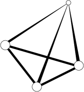
Figure 7: A graph realised as a network of wires embedded in $3d$.

Let us think of the classical graph that we wish to quantise as a network or web of wires set up in our ideal laboratory, see figure 7. To quantise this system using the Dirac operator we must introduce pairs of spinors propagating in both directions along the wires. At the vertices changes in the composition of the spinor pairs are described by elements $u_{bc}\in{\mathrm{SU(2)}}$, $c$ labels the incoming classical bond and $b$ the outgoing bond. These elements $u_{bc}$ necessarily depend on the pair of wires under consideration, $u_{bc}\neq u_{de}$. This is not a feature of the usual Schrödinger quantisation [16, 17] where all wires meeting at a vertex are treated equivalently. It is therefore fair to ask whether our model web could really distinguish bonds in such a way.

One simple geometric argument connecting the matrices $u_{bc}$ to our experimental network is provided by the double covering map $f:{\mathrm{SU(2)}}\rightarrow{\mathrm{SO(3)}}$. Let $R(\theta_{bc})\in{\mathrm{SO(3)}}$ describe the rotation from bond $c$ to $b$ at a vertex. Setting $u_{bc}=f^{-1}(R(\theta_{bc}))$, with some choice of the branch $f^{-1}({\mathrm{SO(3)}})$, we define a set of elements of ${\mathrm{SU(2)}}$ from the architecture of the network. This construction is time-reversal symmetric as $u_{cb}=u_{bc}^{-1}$. (To write this in the form used for the vertex boundary conditions (6.4) choose a reference direction at each vertex and take the $v$ elements $u_{c}$ to be $f^{-1}(R(\theta_{c}))$ where $R(\theta_{c})$ rotates from the reference direction to bond $c$.) We have not attempted to provide a physical justification for this transformation of spinor pairs at the vertices. Our formulation rather shows that the extent to which bonds must be distinguished when quantising a graph with the Dirac operator remains consistent with the picture of the graph as a simple ideal quantum system. There is sufficient geometrical information in the structure of a graph embedded in three dimensions to determine rotations of the spinors at the vertices.

Acknowledgments

We would like to thank Stefan Keppeler for useful discussions and Arnd Bäcker for advice with the numerics. This work has been fully supported by the European Commission under the Research Training Network (Mathematical Aspects of Quantum Chaos) no. HPRN-CT-2000-00103 of the IHP Programme.

References

- [1] V. Alonso and S. De Vincenzo. General boundary conditions for a Dirac particle in a box and their non-relativistic limits. J. Phys. A: Math. Gen., 30:8573–8585, 1997.
- [2] G. Berkolaiko and J. P. Keating. Two-point spectral correlations for star graphs. J. Phys. A: Math. Gen., 32:7827–7841, 1999.
- [3] G. Berkolaiko, H. Schanz, and R. S. Whitney. Form factor for a family of quantum graphs: An expansion to third order. preprint, 2002.
- [4] G. Berkolaiko, H. Schanz, and R. S. Whitney. Leading off-diagonal correction to the form factor of large graphs. Phys. Rev. Lett., 82:104101, 2002.
- [5] M. V. Berry. Semiclassical theory of spectral rigidity. Proc. Roy. Soc. Lond. A, 400:229–251, 1985.
- [6] O. Bohigas, M.-J. Giannoni, and C. Schmit. Characterization of chaotic quantum spectra and universality of level fluctuation laws. Phys. Rev. Lett., 52:1–4, 1984.
- [7] J. Bolte and S. Keppeler. Semiclassical time evolution and trace formula for relativistic spin- particles. Phys. Rev. Lett., 81:1987–1991, 1998.
- [8] J. Bolte and S. Keppeler. A semiclassical approach to the Dirac equation. Ann. Phys. (N.Y.), 274:125–162, 1999.
- [9] J. Bolte and S. Keppeler. Semiclassical form factor for chaotic systems with spin . J. Phys. A: Math. Gen., 32:8863–8880, 1999.
- [10] W. Bulla and T. Trenkler. The free Dirac operator on compact and noncompact graphs. J. Math. Phys., 31:1157–1163, 1990.
- [11] E. Caurier and B. Grammaticos. Extreme level replulsion for chaotic quantum Hamiltonians. Phys. Lett. A, 136:387–390, 1989.
- [12] F. R. Gantmacher. The Theory of Matrices. Chelsea, 1959.
- [13] F. Haake. Quantum Signatures of Chaos. Springer, 1992.
- [14] S. Keppeler, J. Marklof, and F. Mezzadri. Quantum cat maps with spin . Nonlinearity, 14:719–738, 2001.
- [15] V. Kostrykin and R. Schrader. Kirchoff’s rule for quantum wires. J. Phys. A: Math. Gen., 32:595–630, 1999.
- [16] T. Kottos and U. Smilansky. Quantum chaos on graphs. Phys. Rev. Lett., 79:4794, 1997.
- [17] T. Kottos and U. Smilansky. Periodic orbit theory and spectral statistics for quantum graphs. Ann. Phys. (N.Y.), 274:76, 1999.
- [18] J.-P. Roth. Spectre du laplacien sur un graphe. C. R. Acad. Sc. Paris Série I, 296:793–795, 1983.
- [19] R. Scharf. Kicked rotator for a spin . J. Phys. A: Math. Gen., 22:4223–4242, 1989.
- [20] R. Scharf, B. Dietz, M. Kuś, F. Haake, and M. V. Berry. Kramers’ degeneracy and quartic level repulsion. Europhys. Lett., 5:383–389, 1988.
- [21] M. Thaha, R. Blümel, and U. Smilansky. Symmetry breaking and localization in the quantum chaotic regime. Phys. Rev. E, 48:1764–1781, 1993.
- [22] B. Thaller. The Dirac Equation. Springer, 1992.