Boundary effects in the stepwise structure of the Lyapunov spectra for quasi-one-dimensional systems

Abstract

Boundary effects in the stepwise structure of the Lyapunov spectra and the corresponding wavelike structure of the Lyapunov vectors are discussed numerically in quasi-one-dimensional systems consisting of many hard-disks. Four kinds of boundary conditions constructed by combinations of periodic boundary conditions and hard-wall boundary conditions are considered, and lead to different stepwise structures of the Lyapunov spectra in each case. We show that a spatial wavelike structure with a time-oscillation appears in the spatial part of the Lyapunov vectors divided by momenta in some steps of the Lyapunov spectra, while a rather stationary wavelike structure appears in the purely spatial part of the Lyapunov vectors corresponding to the other steps. Using these two kinds of wavelike structure we categorize the sequence and the kinds of steps of the Lyapunov spectra in the four different boundary condition cases.

I Introduction

Chaos is one of the essential concepts to justify a statistical treatment of deterministic dynamical systems. In a chaotic system a small initial error diverges exponentially, as characterized quantitatively by the Lyapunov exponents $\lambda_{n}$, and it means that it is impossible in principle to predict precisely any quantity of deterministic systems at any time and a statistical treatment of the systems is required. It is well known that even one-particle systems can be chaotic and have some of the important statistical properties of equilibrium statistical mechanics such as the mixing property, etc. For this reason many works on the subject of chaos have been done in one-particle systems, for example, billiard systems and Lorentz gas models Gas98 ; Dor99 . However many-particle effects should still play an important role in some statistical aspects, such as the central limit theorem and a justification of thermodynamical reservoirs, etc. Therefore it should be interesting to know what happens with the combination of a chaotic effect and a many-particle effect, in other words, to know which chaotic effects do not appear in one-particle systems.

The Lyapunov spectrum is introduced as the sorted set $\{\lambda_{1},\lambda_{2},\cdots\}$ of Lyapunov exponents satisfying the condition $\lambda_{1}\geq\lambda_{2}\geq\cdots$, and is a quantity to characterize the many-particle chaotic dynamics. Recently a stepwise structure of the Lyapunov spectrum was reported numerically, as one of the many-particle chaotic effects, in many-disk systems in which each disk interacts with the other disks by hard-core interactions Del96 ; Mil98a ; Pos00 . This stepwise structure appears in the region of small absolute values of Lyapunov exponents. This fact suggests that steps in the Lyapunov spectra come from slow and macroscopic behavior of the system, because small positive Lyapunov exponents should correspond to slow relaxation precesses. This point is partly supported by the existence of a global structure in the Lyapunov vectors, the so called Lyapunov modes, which are wavelike structures in the tangent space of each eigenvector of a degenerate Lyapunov exponent, that is, for each stepwise structure Mil98a ; Pos00 ; Mcn01a ; Pos02a . The wavelike structure of the Lyapunov vectors appears as a function of the particle position, so this structure is also important as a relation to connect the tangent space with the phase space. Although the Lyapunov vectors have been the subject of some works more than a decade ago (for example, see Refs. Kan86 ; Ike86 ; Gol87 ; Kon92 ; Fal91 ; Yam98 ; Pik01 ; Yam02 ), it is remarkable that an observation of their global structure in fully chaotic many-particle systems has only recently appeared. Explanations for the stepwise structure of the Lyapunov spectra have been attempted using periodic orbit models Tan01 and using the master equation approach Tan02 . Other approaches to the Lyapunov modes have included using a random matrix approach for a one-dimensional model Eck00 and using a kinetic theoretical approach Mcn01b , by considering these as the ”Goldstone modes” Wij02 .

If the stepwise structure of Lyapunov spectra is a reflection of a global behavior of the system, then one may ask the question: Does such a structure depend on boundary conditions which specify the global structure of the system? One of the purposes of this paper is to answer this question using some simple examples. In this paper we investigate numerically the stepwise structure of the Lyapunov spectra in many-hard-disk systems of two-dimensional rectangular shape with the four kinds of the boundary conditions: [A1] purely periodic boundary conditions, [A2] periodic boundary conditions in the $x$-direction and hard-wall boundary conditions in the $y$-direction, [A3] hard-wall boundary conditions in the $x$-direction and periodic boundary conditions in the $y$-direction, and [A4] purely hard-wall boundary conditions. In all cases we took the $y$-direction as the narrow direction of the rectangular shape of the system and $x$-direction as the longer orthogonal direction. The case [A1] means that the global shape of the system is like the surface of a doughnut shape, the cases [A2] and [A3] means that the system has the shape of the surface of pipe with hard-walls in its ends. Case [A2] is a long pipe with small diameter while case [A3] is a short pipe with a large diameter. The case [A4] means that the system has just a rectangular shape surrounded by hard-walls. Adopting hard-wall boundary conditions in a particular direction destroys the total momentum conservation in that direction, so by considering these models we can investigate the effects of the total momentum conservation on the stepwise structure of the Lyapunov spectra and the Lyapunov modes. This can be used to check some theoretical approaches to these phenomena like those in Refs. Tan02 ; Eck00 ; Mcn01b , in which the total momentum conservation plays an essential role in explaining the stepwise structure of the Lyapunov spectra or the Lyapunov modes. We obtain different stepwise structures of the Lyapunov spectra with each different boundary condition case. Especially, we observe a stepwise structure of the Lyapunov spectrum even in the purely hard-wall boundary case [A4], in which the total momentum is not conserved in any direction.

The second purpose of this paper is to categorize the stepwise structure of the Lyapunov spectra according to the wavelike structure of the Lyapunov vectors. So far wavelike structure of the Lyapunov vectors was reported in the Lyapunov vector components as a function of positions, for example in the quantity $\delta q_{yj}^{(n)}$ as a function of the position $q_{xj}$ (the transverse Lyapunov mode) Mil98a ; Pos00 ; Mcn01a and in the quantity $\delta q_{xj}^{(n)}$ as a function of the position $q_{xj}$ (the longitudinal Lyapunov mode) Pos02 , in which $\delta q_{yj}^{(n)}$ ($\delta q_{xj}^{(n)}$) is the $y$-component ($x$-component) of the spatial coordinate part of the Lyapunov vector of the $j$-th particle corresponding to the $n$-th Lyapunov exponent $\lambda_{n}$, and $q_{xj}$ is the $x$-component of the spatial component of the $j$-th particle. These wavelike structures appear in the stepwise region of the Lyapunov spectrum. However it is not clear whether there is a direct connection between the sequence and the kinds of steps of the Lyapunov spectrum and the modes of wavelike structure of the Lyapunov vectors in the numerical studies, that is, how we can categorize the steps of the Lyapunov spectrum by the Lyapunov modes. In this paper we show another type of wavelike structure of the Lyapunov vectors, which appears in the quantity $\delta q_{yj}^{(n)}/p_{yj}$ with the $y$-component $p_{yj}$ of the momentum coordinate of the $j$-th particle, and use this wavelike structure to categorize the stepwise structure of the Lyapunov spectra. The Lyapunov vector components $\delta q_{xj}^{(n)}$, $\delta q_{yj}^{(n)}$ and $\delta q_{yj}^{(n)}/p_{yj}$ have a common feature in which each quantity gives a constant corresponding to one of the zero Lyapunov exponents of the system with purely periodic boundary conditions, because of the conservation of center of mass or the deterministic nature of the orbit. More concretely in this paper we consider the two kinds of graphs: [B1] the quantity $\delta q_{yj}^{(n)}$ as a function of the position $q_{xj}$, namely the transverse Lyapunov mode, and [B2] the quantity $\delta q_{yj}^{(n)}/p_{yj}$ as a function of the position $q_{xj}$ and time (or collision number). In the two-dimensional rectangular systems consisting of many-hard-disks with periodic boundary conditions (the boundary case [A1]) it is known that there are two types of steps of the Lyapunov spectra: steps consisting of two Lyapunov exponents and steps consisting of four Lyapunov exponents Pos00 ; Mcn01a . The wavelike structure in the graph [B1] corresponding to the two-point steps of the Lyapunov spectrum for such a rectangular system is well known. In this paper we show the wavelike structure corresponding to the four-point steps of the Lyapunov spectrum in the graph [B2]. Besides, we observe time-dependent oscillations in the graph [B2], whereas the graph [B1] is rather stationary in time. The wavelike structure in the graph [B2] also appears in the rectangular systems with a hard-wall boundary condition (the boundary cases [A2], [A3] and [A4]), specifically even in the case of purely hard-wall boundary conditions in which the transverse Lyapunov mode [B1] does not appear. We show that the stepwise structure of the Lyapunov spectra in the boundary cases [A1], [A2], [A3] and [A4] can be categorized by the wavelike structures of the graphs [B1] and [B2].

One of the problems which make it difficult to investigate the structure of the Lyapunov spectra and the Lyapunov modes is that the calculation of a full Lyapunov spectra for many-particle system is a very time-consuming numerical calculation. Therefore it should be important to know how we can calculate the stepwise structure of the Lyapunov spectra and the Lyapunov modes with as little calculation time as possible. It is known that a rectangular system has a wider stepwise region of the Lyapunov spectrum than a square system Pos00 . Noting this point, in this paper we concentrate on the most strongly rectangular system, namely on the quasi-one-dimensional system in which the rectangle is too narrow to allow particles to exchange their positions. As will be shown in this paper, the stepwise structure of the Lyapunov spectrum for the quasi-one-dimensional system is the same as the fully rectangular system which allows exchange of particle positions and each particle can collide with any other particle, and the steps of the Lyapunov spectra consist of two-point steps and four-point steps in the periodic boundary case [A1]. We also determine an appropriate particle density to give clearest stepwise structure of the Lyapunov spectrum in the quasi-one-dimensional system.

The outline of this paper is as follows. In Sect. II we discuss how we can get the stepwise structure of the Lyapunov spectra for a small number of particle systems with a quasi-one-dimensional shape. The density dependence of the Lyapunov spectrum for the quasi-one-dimensional system is investigated to get a clearly visible stepwise structure of the Lyapunov spectra. In Sect. III we consider the purely periodic boundary case (the boundary case [A1]), and investigate wavelike structures in the graphs [B1] and [B2] of Lyapunov vector components. In Sect. IV we consider the cases including a hard-wall boundary condition (the boundary cases [A2], [A3] and [A4]) with calculations of the graphs [B1] and [B2], and compare the stepwise structures of the Lyapunov spectra and the wavelike structures in the graphs [B1] and [B2] in the above four boundary cases. Finally we give our conclusion and remarks in Sect. V.

II Quasi-one-dimensional systems and density dependence of the Lyapunov spectrum

The stepwise structure of the Lyapunov spectra is purely a many-particle effect of the chaotic dynamics, and so far it has been investigated in systems of 100 or more particles. However the numerical calculation of Lyapunov spectra for such large systems is not so easy even at present. Noting this point, in this section we discuss briefly how we can investigate the stepwise structure of the Lyapunov spectrum for a system whose number of particles is as small as possible. We also discuss what is a proper particle density to get clear steps of the Lyapunov spectrum. These discussions give reasons to choose some values of system parameters used in the following sections.

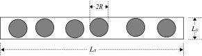
Figure 1: Quasi-one-dimensional system: A narrow rectangular system satisfying the conditions $2RN<L_{x}$ and $2R<L_{y}<4R$.

We consider two-dimensional systems consisting of $N$ number of hard-disks in which the radius of the particle is $R$ and the width (height) of the system is $L_{x}$ ($L_{y}$). One way to get the stepwise structure of Lyapunov spectrum in a two-dimensional system consisting of a small number of particles is to choose a rectangular system rather than a square system, because the stepwise region in the Lyapunov spectrum is wider in a more rectangular system rather than in a square system even if the number of particles is the same Pos00 . Noting this characteristic, we concentrate on the most rectangular case, namely the quasi-one-dimensional system defined by the conditions

$$2RN<L_{x}\;\;\mbox{and}\;\;2R<L_{y}<4R.$$ (1)

A schematic illustration of the quasi-one-dimensional system is shown in Fig. 1. In other words, the quasi-one-dimensional system is introduced as a narrow rectangular system where each particle can interact with two nearest-neighbor particles only and particles do not exchange the order of their positions. In the quasi-one-dimensional system the upper bound $\rho_{max}$ of the particle density $\rho\equiv N\pi R^{2}/L_{x}L_{y}$ is given by $\rho_{max}=\pi/4=0.7853\cdots$. In such a system we can get a stepwise structure of the Lyapunov spectrum even in a 10-particle system ($N=10$), as shown in Fig. 2, which is the Lyapunov spectrum normalized by the maximum Lyapunov exponent $\lambda_{1}\approx 3.51$. To get this figure we chose the parameters as $R=1$, $L_{y}=2R\times(1+10^{-6})$, $L_{x}=NL_{y}\times(1+10^{-3})$, and the mass $M$ of the particle and the total energy $E$ are given by $1$ and $N$, respectively, and we used periodic boundary conditions in both the directions. The particle density of this system is given by $\rho=0.7846\cdots$. Noting the pairing property of the Lyapunov spectrum for Hamiltonian systems, namely the property that in Hamiltonian systems any positive Lyapunov exponent accompanies a negative Lyapunov exponent with the same absolute value Arn89 ; Gas98 , we plotted the first half of the Lyapunov spectrum in Fig. 2. (The same omission of the negative branch of Lyapunov spectra from plots will be used throughout this paper.) It is clear that the Lyapunov exponents $\lambda_{16}$ and $\lambda_{17}$ form a two-point step in this Lyapunov spectrum.

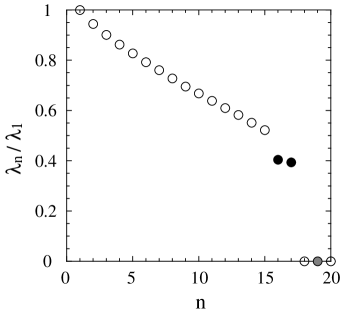
Figure 2: Lyapunov spectrum normalized by the maximum Lyapunov exponent in a 10-hard-disk system with the periodic boundary conditions in both directions. The Lyapunov exponents $\lambda_{16}$ and $\lambda_{17}$ shown as the black circles form a two-point step accompanying the transverse Lyapunov modes shown in Fig. 3. The gray circle is the zero-Lyapunov exponent $\lambda_{19}$ whose corresponding Lyapunov vector components $\delta q_{yj}^{(n)}$ show a constant behavior (also see Fig. 3).

In order to calculate Lyapunov spectra and Lyapunov vectors we use the algorithm due to Benettin et al., which is characterized by intermittent rescaling and renormalization of Lyapunov vectors Ben76 ; Shi79 . In the application of this algorithm to systems with hard-core particle interactions, we calculate the matrix $\Lambda(t_{k})$, whose column vectors give the Lyapunov vectors $\delta\mathbf{\Gamma}_{n}(t_{k})$ corresponding to the local-time Lyapunov exponent $\tilde{\lambda}_{n}(t_{k})$ at time $t=t_{k}$ just after the $k$-th collision of particles. The dynamics of the matrix $\Lambda(t_{k})$ is given by $\Lambda(t_{k+1})=\mathcal{N}_{k}\mathcal{G}_{k}\mathcal{M}_{k}\Lambda(t_{k})$, in which $\mathcal{N}_{k}$ is the matrix required to normalize each column vector of the operated matrix, $\mathcal{G}_{k}$ is the Gram-Schmidt procedure ensuring the orthogonality of the columns of the operated matrix, and $\mathcal{M}^{(k)}$ specifies the tangent space dynamics including a free flight and a particle collision Del96 . The local-time Lyapunov exponent $\tilde{\lambda}_{n}(t_{k})$ is calculated as the exponents of the exponential divergence (contraction) from the $n$-th column vectors of the matrix $\Lambda(t_{k})$ to the $n$-th column vectors of the matrix $\mathcal{G}_{k}\mathcal{M}_{k}\Lambda(t_{k})$. The Lyapunov exponent $\lambda_{n}$ is given as a time-averaged local-time Lyapunov exponent after a long time calculation: $\lambda_{n}=\lim_{k\rightarrow\infty}\tilde{\lambda}_{n}(t_{k})$. Here we use the standard metric $d\delta s^{2}=\sum_{j=1}^{N}[d\delta q_{xj}^{(n)}{}^{2}+d\delta q_{yj}^{(n)}{}^{2}+d\delta p_{xj}^{(n)}{}^{2}+d\delta p_{yj}^{(n)}{}^{2}]$ for the tangent space with the $x$-component $\delta p_{xj}^{(n)}$ and $y$-component $\delta p_{yj}^{(n)}$ of the Lyapunov vector of the $j$-th particle corresponding to the local-time Lyapunov exponent $\tilde{\lambda}_{n}$. Other articles such as Refs. Ben76 ; Shi79 ; Del96 should be referred to for more details of the Benettin algorithm and the tangent space dynamics of many-hard-disk systems.

It is very important to note that there are two ways that convince us of the structure of the Lyapunov spectrum; one is simply to find a step structure directly in the Lyapunov spectrum, and another is to find a structure in the Lyapunov vectors corresponding to specific Lyapunov exponents. Fig. 3 is the plot of the time-average $\langle\delta q_{yj}^{(n)}\rangle$ of the $y$-component of the $j$-th particle of the spatial part of the Lyapunov vector $\delta\mathbf{\Gamma}_{n}$ corresponding to the Lyapunov exponents $\lambda_{n}$, for $n=19,17$ and $16$ as functions of the time-average $\langle q_{xj}\rangle/L_{x}$ of the normalized $x$-component of spatial coordinate of the $j$-th particle ($j=1,2,\cdots,N$) (the graph [B1]). The corresponding Lyapunov exponents $\lambda_{17}$ and $\lambda_{16}$ are shown as the black-filled circles in Fig. 2 and construct a two-point step of the Lyapunov spectrum. To take the time average of the quantities $\delta q_{yj}^{(n)}$ and $q_{xj}$ we picked up these values just after particle collisions over $100N$ collisions and take the arithmetic averages of them. The step consisting of two points in the Lyapunov spectrum of Fig. 2 accompanies wavelike structures in their Lyapunov vectors, which are called the transverse Lyapunov modes. It should be emphasized that the Lyapunov modes in Fig. 3 are rather stationary over $100N$ particle collisions and to take the time average can be a useful way to get clear their wavelike structures. In this figure we fitted the numerical data for the Lyapunov modes corresponding to the Lyapunov exponents $\lambda_{n}$, $n=17$ and $16$, to the function $y=\alpha_{n}\cos(2\pi x+\beta_{n})$ ($(\alpha_{17},\beta_{17})=(0.19913,0.9703)$ for the triangle dots, and $(\alpha_{16},\beta_{16})=(0.24025,-0.59677)$ for the square dots). It should be noted that the difference $\beta_{17}-\beta_{16}=0.9703-(-0.59677)=1.56707$ of the two values of the phases $\beta_{n}$ is approximately $\pi/2=1.570\cdots$, meaning that these two waves are orthogonal with each other. The graph of the Lyapunov vector component $\delta q_{yj}^{(n)}$ as a function of the position $q_{xj}$ ($j=1,2,\cdots,N$) become constant in one of the zero Lyapunov exponent $\lambda_{19}$ shown as the gray-filled circle in Fig. 2. In Fig. 3 we also fitted the numerical data corresponding to the zero-Lyapunov exponent $\lambda_{19}$ by the constant function $y=\alpha_{19}$ with the fitting parameter value $\alpha_{19}=0.015114$.

Figure 3: Time-averaged $y$-components $\langle\delta q_{yj}^{(n)}\rangle$ of the spatial part of the Lyapunov vector of the $j$-th particle as functions of the time-average $\langle q_{xj}\rangle/L_{x}$ of the normalized $x$-component of spatial coordinate of the $j$-th particle corresponding to the Lyapunov exponents $\lambda_{n}$, $n=19,17$ and $16$, in the 10-hard-disk system with the periodic boundary conditions in both directions. The circle, triangle and square dots correspond to the Lyapunov exponents $\lambda_{19}$, $\lambda_{17}$ and $\lambda_{16}$, respectively, which are shown as the black- and gray-filled circles in Fig. 2. The dotted and broken lines are the fitting lines for the sinusoidal functions, and the solid line is the fitting for the constant function.

Although we can recognize the two-point step of the Lyapunov spectrum in Fig. 2, it is important to note that there is another type of steps in the two-dimensional hard-disk system with a rectangular shape and periodic boundary conditions. It is well known that in such a system the Lyapunov spectrum can have a stepwise structure consisting of two-point steps and four-point steps Pos00 ; Mcn01b . If we want to investigate the four-point steps of the Lyapunov spectrum we may have to consider a system consisting of more than 10 particles.

Now we mention an angle in components of the Lyapunov vectors. Fig. 4 is the graph for the time-average $\langle\theta_{n}\rangle$ of the angle $\theta_{n}$ between the spatial part $\delta\mathbf{q}^{(n)}$ and the momentum part $\delta\mathbf{p}^{(n)}$ of the Lyapunov vector $\delta\mathbf{\Gamma}_{n}=(\delta\mathbf{q}^{(n)},\delta\mathbf{p}^{(n)})^{T}$ where ^T is the transverse operation, and $\theta_{n}$ is defined by

$$\theta_{n}\equiv\cos^{-1}\left(\frac{\delta\mathbf{q}^{(n)}\cdot\delta\mathbf{p}^{(n)}}{|\delta\mathbf{q}^{(n)}||\delta\mathbf{p}^{(n)}|}\right),$$ (2)

except for the ones corresponding to the zero Lyapunov exponents. Here in order to take the time-average of the angle $\theta_{n}$ we picked up its values just after particle collisions over $1000N$ collisions and took the arithmetic average of them. This graph shows that the spatial part $\delta\mathbf{q}^{(n)}$ and the momentum part $\delta\mathbf{p}^{(n)}$ of the Lyapunov vector are pointed toward almost the same direction, especially for the Lyapunov vectors corresponding to small absolute values of Lyapunov exponents Mcn01b . This fact suggests that if we get a structure in the vector $\delta\mathbf{q}^{(n)}$ then we may get the similar structure in the vector $\delta\mathbf{p}^{(n)}$, and vice versa. It should also be noted that this gives a justification for some approaches to Lyapunov exponents in which the Lyapunov exponents are calculated through the spatial coordinate part only (or the momentum part only) of the Lyapunov vector Bei98 ; Tan01 . We may also note that the graph for $\theta_{n}$, $n=1,2,\cdots,2N-3$ and $\theta_{4N-n+1}$, $n=1,2,\cdots,2N-3$ are symmetric with respect to the line $y=1/2$, which comes from the symplectic property of the Hamiltonian dynamics.

Figure 4: Time-averaged angle $\langle\theta_{n}\rangle$ between the spatial part $\delta\mathbf{q}^{(n)}$ and the momentum part $\delta\mathbf{p}^{(n)}$ of the Lyapunov vector $\delta\mathbf{\Gamma}_{n}=(\delta\mathbf{q}^{(n)},\delta\mathbf{p}^{(n)})^{T}$ corresponding to the Lyapunov exponent $\lambda_{n}$ in the 10-hard-disk system with the periodic boundary conditions in both directions.

Another important point to get a clear stepwise structure for the Lyapunov spectrum in a small system is to choose a proper particle density of the system. Even if we restrict our consideration to quasi-one-dimensional systems, the shape of the Lyapunov spectrum depends on the particle density, so we should choose a density that gives a clearly visible stepwise structure in the Lyapunov spectrum. Fig. 5(a) is the Lyapunov spectra normalized by the maximum Lyapunov exponents for quasi-one-dimensional systems consisting of 50 hard-disks ($N=50$) with periodic boundary conditions in both directions. We also give an enlarged figure 5(b) for the small Lyapunov exponent region. Here the system parameters are given by $R=1$, $L_{y}=2R(1+10^{-6})$, $L_{x}=NL_{y}(1+d)$, and we used the case of $M=1$ and $E=N$. The five Lyapunov spectra correspond to the case of $d=10^{-4}$ (the circle dots, the density $\rho=0.7853\cdots$), the case of $d=10^{-1}$ (the triangle dots, the density $\rho=0.7139\cdots$), the case of $d=1$ (the square dots, the density $\rho=0.3926\cdots$), the case of $d=10$ (the diamond dots, the density $\rho=0.07139\cdots$), the case of $d=10^{2}$ (the upside-down triangle dots, the density $\rho=0.007776\cdots$). The maximum Lyapunov exponents $\lambda_{1}$ are given approximately by $3.62$, $2.44$, $0.934$, $0.279$ and $0.0579$ in the cases of $d=10^{-4},10^{-1},1,10$ and $10^{2}$, respectively. As shown in Figs. 5(a) and (b), for smaller values of the quantity $d$ (namely in the higher particle density) the gaps between the nearest steps of the Lyapunov spectrum become larger, although the stepwise region of the Lyapunov spectrum does not seem to depend on the quantity $d$. This means that we can get a clear stepwise structure of the Lyapunov spectrum in the small $d$ case (namely at high density).

Figure 5: Density dependence of Lyapunov spectrum normalized by the maximum Lyapunov exponent for quasi-one-dimensional systems consisting of 50 particles with the periodic boundary conditions in both directions. The five Lyapunov spectra correspond to the case of $L_{y}=2R(1+10^{-6})$, $L_{x}=NL_{y}(1+d)$ with $d=10^{-4}$ (the circle dots), the case of $d=10^{-1}$ (the triangle dots), the case of $d=1$ (the square dots), the case of $d=10$ (the diamond dots), the case of $d=10^{2}$ (the upside-down triangle dots). (a) Full scale. (b) A small positive Lyapunov exponent region including the stepwise structure of the Lyapunov spectra. In the figure (b) we filled dots by black (gray) for the Lyapunov exponents whose corresponding time-averaged Lyapunov vector components $\langle\delta q_{yj}^{(n)}\rangle$ of the spatial part of the Lyapunov vector of the $j$-th particle as functions of the time-averaged $x$-component $\langle q_{xj}\rangle$ of spatial coordinate of the $j$-th particle show wavelike structures (constant behaviors).

In Fig. 5(b) the Lyapunov exponents accompanying wavelike structures (constant behaviors) in the time-averaged Lyapunov vector components $\langle\delta q_{yj}^{(n)}\rangle$, as functions of the position $\langle q_{xj}\rangle$, are shown as the dots blacked (grayed) out. In the small $d$ case, looking from the zero Lyapunov exponents, the two-point step appears first (see the cases of $d=10^{-4},10^{-1}$ and $1$ in Fig. 5(b)), whereas the four-point step appears first in the large $d$ case (see the cases of $d=10^{1}$ and $d=10^{2}$ in Fig. 5(b)). Besides, at least in the small $d$ case, the two-point steps and the four-point steps do not appear repeatedly (see the cases of $d=10^{-4}$ and $10^{-1}$ in Fig. 5(b)). These facts mean that the sequence of steps in the Lyapunov spectrum depends on the quantity $d$, namely the particle density.

Wavelike structures in the time-averaged Lyapunov vector components $\langle\delta q_{yj}^{(n)}\rangle$ as functions of the position $\langle q_{xj}\rangle$, namely the transverse Lyapunov modes, appear mainly in two-point steps of the Lyapunov spectra. Therefore we can use these wavelike structures to distinguish two-point steps from four-point steps of the Lyapunov spectra. However such a distinguishability sometimes seems to fail in steps of the Lyapunov spectra near a region where the Lyapunov spectra is changing smoothly. Actually the transverse Lyapunov modes may appear even in some four-point steps, if they are near such a smoothly changing Lyapunov spectrum region. On the other hand, in such a region of the Lyapunov spectra, fluctuation of Lyapunov vectors is rather large, and the wavelike structure of the Lyapunov vectors become vague. In Fig. 5(b) we did not indicate by black-filled dots the Lyapunov exponents whose corresponding Lyapunov vector components $\langle\delta q_{yj}^{(n)}\rangle$ as functions of the position $\langle q_{xj}\rangle$ show wavelike-structures with such a level of vagueness.

Based on the discussions in this section, in the following two sections we consider only the case whose system parameters are given by $N=75$, $R=1$, $M=1$ and $E=N$. The height and the width of the system are given by $L_{y}=2R(1+10^{-6})$ and $L_{x}=1.5NL_{y}$ (the density $\rho=0.5235\cdots$) in the purely periodic boundary case considered in the next section. In this case, as will be shown in the next section, we can recognize at least 2 clear four-point steps, and the two-point steps and the four-point steps of the Lyapunov spectrum appear repeatedly in the first few steps in the Lyapunov spectrum for the system with the purely periodic boundary conditions. We always take the time averaged quantities $\langle\delta q_{yj}^{(n)}\rangle$ and $\langle q_{xj}\rangle$ of the quantities $\delta q_{yj}^{(n)}$ and $q_{xj}$, respectively as the arithmetic average of their values taken in the times immediately after particle collisions, over $100N$ collisions. We calculated more than $2\times 10^{5}$ collisions ($10^{6}$ collisions in some of the models) in order to get the Lyapunov spectra and the Lyapunov vectors in the models considered in this paper.

III Quasi-One-Dimensional Systems with Periodic Boundary Conditions

In this section we consider the Lyapunov spectrum for the quasi-one-dimensional system with periodic boundary conditions in both the directions (the boundary case [A1]). A schematic illustration of this system for latter comparisons is given in Fig. 6 in which the broken line of the boundary means to take the periodic boundary conditions. This system satisfies total momentum conservation in both the directions, and is regarded as a reference model for the models considered in the following section.

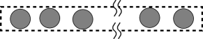
Figure 6: A schematic illustration of a quasi-one-dimensional system with periodic boundary conditions in both directions. The broken lines indicate periodic boundary conditions at that boundary.

Fig. 7 is the small positive Lyapunov exponent region of the Lyapunov spectrum normalized by the maximum Lyapunov exponent $\lambda_{1}\approx 1.33$, including its stepwise region, for a quasi-one-dimensional system with periodic boundary conditions in both the directions. The global shape of the Lyapunov spectrum is given in the inset in this figure. We used the values of the system parameters chosen at the end of the preceding section. At least 5 steps consisting 3 two-point steps and 2 four-point steps are clearly visible in this Lyapunov spectrum.

Figure 7: The stepwise structure of the Lyapunov spectrum normalized by the maximum Lyapunov exponent for a quasi-one-dimensional system with periodic boundary conditions in both directions. Inset: Full scale for the normalized Lyapunov spectrum. The circular dots are filled by black (gray) in the Lyapunov exponents corresponding to wavelike structures (a constant behavior) of the time-averaged Lyapunov vector components $\langle\delta q_{yj}^{(n)}\rangle$ shown in Fig. 8.

The two-point steps of the Lyapunov spectrum accompany wavelike structures in their corresponding Lyapunov vectors. Fig. 8 is the graphs of the time-averaged Lyapunov vector components $\langle\delta q_{yj}^{(n)}\rangle$ corresponding to the Lyapunov exponent $\lambda_{n}$, $n=149,147,146,141$ and $140$ as functions of the time-averaged position component $\langle q_{xj}\rangle$ normalized by the length $L_{x}$ (the graph [B1]). The Lyapunov exponents used for this figure are shown as the black or gray circles in Fig. 7. In this figure we also gave fittings of the numerical data by sinusoidal equations and a constant function. The fitting equations are $y=\alpha_{n}\cos(2\pi x+\beta_{n})$ for $n=147,146$ ( $(\alpha_{147},\beta_{147})=(-0.16132,-4.5575),\;(\alpha_{146},\beta_{146})=(-0.16125,0.14928)$ ), and $y=\alpha_{n}\cos(4\pi x+\beta_{n})$ for $n=141,140$ ( $(\alpha_{141},\beta_{141})=(-0.15775,-0.30581),\;(\alpha_{140},\beta_{140})=(0.15782,1.2666)$ ). Concerning these fitting parameters, it is important to note the relations $|\alpha_{147}|\approx|\alpha_{146}|$, $|\alpha_{141}|\approx|\alpha_{140}|$, $\beta_{146}-\beta_{147}\approx 3\pi/2$ and $\beta_{140}-\beta_{141}\approx\pi/2$, meaning that the two wavelike structures in the same two-point step are orthogonal to each other. In Fig. 8 we also draw a graph of the averaged Lyapunov vector component $\langle\delta q_{yj}^{(n)}\rangle$ as a function of the normalized position $\langle q_{xj}\rangle/L_{x}$ corresponding to the second zero Lyapunov exponent $\lambda_{149}$, which is roughly speaking constant, and is fitted by a constant function $y=\alpha_{149}$ with the fitting parameter value $\alpha_{149}=0.018901$. These results suggest a conjecture for the approximate form of the Lyapunov vector component $\delta q_{yj}^{(n(k))}$ corresponding to the Lyapunov exponents $\lambda_{n(k)}$ and $\lambda_{n(k)-1}$ in the same $k$-th two-point step counting from the zero Lyapunov exponents as

$$\left\{\delta q_{yj}^{(n(k))},\;\delta q_{yj}^{(n(k)-1)}\right\}\approx$$

$$\left\{\alpha_{k}\cos\left(\frac{2\pi k}{L_{x}}q_{xj}+\beta_{k}\right),\;\alpha_{k}\sin\left(\frac{2\pi k}{L_{x}}q_{xj}+\beta_{k}\right)\right\},$$

(3)

$j=1,2,\cdots,N$ with constants $\alpha_{k}$ and $\beta_{k}$. (Note that in this paper we always count the sequence of steps of Lyapunov spectra looking from the zero Lyapunov exponents, so, for example, the two-point step consisting of the Lyapunov exponents $\lambda_{147}$ and $\lambda_{146}$ ($\lambda_{141}$ and $\lambda_{140}$) in the Lyapunov spectrum shown in Fig. 8 is the first (second) two-point step.) It may be noted that the constant $\alpha_{k}$ in Eq. (3) should be determined by the normalization condition of the Lyapunov vector, which is used in the Benettin algorithm to calculate the Lyapunov spectrum and Lyapunov vectors in this paper.

Figure 8: Time-averaged Lyapunov vector components $\langle\delta q_{yj}^{(n)}\rangle$ as functions of the time-average $\langle q_{xj}\rangle/L_{x}$ of the normalized $x$-component of the spatial coordinate of the $j$-th particle corresponding to the $n$-th Lyapunov exponent $\lambda_{n}$ for the quasi-one-dimensional system with the periodic boundary conditions in both directions ($n=149,147,146,141$ and $140$). The corresponding Lyapunov exponents are shown as the black- and gray-filled circles in Fig. 7. The numerical data are fitted by a constant function and sinusoidal functions.

It should be emphasized that the wavelike structures in Figs. 3 and 8 correspond to the two-point steps of the Lyapunov spectrum. We cannot recognize such a clear wavelike structure in the graph of the Lyapunov vector component $\langle\delta q_{yj}^{(n)}\rangle$ as a function of the position $\langle q_{xj}\rangle$ corresponding to the four-point steps of the Lyapunov spectrum. This suggests that the physical meaning of the four-point steps is different from the two-point steps, and we should consider a different quantity to investigate as a structure of Lyapunov vectors corresponding to the four-point steps of the Lyapunov spectrum. Now, as one of the important results of this paper, we show that wavelike structures in the quantities $\delta q_{yj}^{(n)}/p_{yj}$ as functions of $q_{xj}$ and the collision number appear in the four-point steps of the Lyapunov spectrum. As a motivation to introduce the quantity $\delta q_{yj}^{(n)}/p_{yj}$ to investigate its structure, we note that the small perturbation of the spatial coordinates of the particles in the direction of the orbit, namely the small perturbation $\delta\mathbf{q}\propto\mathbf{p}$, leads to a zero-Lyapunov exponent, so that the quantities $\delta q_{yj}^{(n)}/p_{yj}$, $j=1,2,\cdots,N$ should give a constant value corresponding to this zero Lyapunov exponent. This is the common feature as the quantity $\delta q_{yj}^{(n)}$, which shows a constant behavior corresponding to one of the zero-Lyapunov exponents owing to the conservation of center of mass, and whose wavelike structure we have already discussed.

Before showing graphs of the quantities $\delta q_{yj}^{(n)}/p_{yj}$, we discuss some difficulties in the investigation of wavelike structure in these quantities. It is much harder to get the wavelike structure of these quantities corresponding to the four-point steps of the Lyapunov spectrum compared to the quantities $\delta q_{yj}^{(n)}$ corresponding to the two-point steps of the Lyapunov spectrum, for at least two reasons. As the first reason, fluctuation in the wavelike structure of the quantities $\delta q_{yj}^{(n)}/p_{yj}$ is much bigger than in the wavelike structure of the quantities $\delta q_{yj}^{(n)}$, partly because such a fluctuation is magnified in the case of a small absolute value of the quantity $p_{yj}$ appearing in the denominator of the quantity $\delta q_{yj}^{(n)}/p_{yj}$. Secondly, the wavelike structure of the quantity $\delta q_{yj}^{(n)}/p_{yj}$, at least the magnitude of its wave, oscillates periodically in time, whereas the wavelike structure of the quantities $\delta q_{yj}^{(n)}$ in Fig. 8 are stationary at least over more than $100N$ collisions. This fact gives an upper bound on the time period (or the collision number interval) over which we can take the time-average of the quantities $\delta q_{yj}^{(n)}/p_{yj}$ in order to suppress the fluctuations and get their clear wavelike structures. In this paper we express the local time-averages of the quantities $\delta q_{y}^{(n)}/p_{yj}$ and $q_{xj}$ as $\langle\delta q_{yj}^{(n)}/p_{yj}\rangle_{t}$ and $\langle q_{xj}\rangle_{t}$, respectively, with the suffix $t$ to remind us that they can change in time.

Figure 9: Local time-averaged quantities $\langle\delta q_{yj}^{(n)}/p_{yj}\rangle_{t}$ as functions of the normalized position $\langle q_{xj}\rangle_{t}/L_{x}$ and the collision number $n_{t}$ corresponding to (a) the Lyapunov exponent $\lambda_{142}$ in the first four-point step and (b) the Lyapunov exponent $\lambda_{139}$ in the second four-point step in the same collision number interval $[543000,548100]$. The system is the quasi-one-dimensional system with the periodic boundary conditions in both directions, and the corresponding Lyapunov exponents are indicated by arrows in Fig. 7. In the contour plots on the bottoms of these three-dimensional plots, red dotted lines, black solid lines and blue broken lines correspond to the values $\langle\delta q_{yj}^{(n)}/p_{yj}\rangle_{t}=0.08,0$ and $-0.08$, respectively.

Figure 10: Contour plots of the local-time averaged quantities $\langle\delta q_{yj}^{(n)}/p_{yj}\rangle_{t}$ as functions of the normalized position $\langle q_{xj}\rangle_{t}/L_{x}$ and the collision number $n_{t}$ corresponding to the first four-point step consisting of the Lyapunov exponents $\lambda_{n}$, $n=145,144,143$ and $142$ in the same collision number interval $[538500,548100]$. Here red dotted lines, black solid lines and blue broken lines correspond to the values $\langle\delta q_{yj}^{(n)}/p_{yj}\rangle_{t}=0.08,0$ and $-0.08$, respectively. The system is the quasi-one-dimensional system with the periodic boundary conditions in both directions, and the corresponding Lyapunov exponents used in this figure are indicated by the brace under circles in Fig. 7.

In this and the next sections we will give the many graphs of $\delta q_{yj}^{(n)}/p_{yj}$ as functions of $q_{xj}$ and the collision number by taking their local time-averages, so here we summarize how we calculate the data for those graphs from a technical point of view. First we take the arithmetic time-average $\langle\delta q_{yj}^{(n)}/p_{yj}\rangle_{t}$ and $\langle q_{xj}\rangle_{t}$ of the quantities $\delta q_{yj}^{(n)}/p_{yj}$ and $q_{xj}$, respectively, using their values just after particle collisions over $4N$ collisions ($8N$ collisions), but if the absolute value $|p_{yj}|$ of the momentum is less than 10 percent (5 percent) of the averaged momentum amplitudes $\sqrt{2ME/N}$ then we exclude the quantity $\delta q_{yj}^{(n)}/p_{yj}$ at that time from samples to take this local time-average, in the models of this section and the subsection IV.1 (in the models of the subsections IV.2 and IV.3). (Therefore the sample number for taking the arithmetic averages can be less than $4N$ ($8N$) in the models of this section and the subsection IV.1 (in the models of the subsections IV.2 and IV.3).) On this local time-averages we can still get more than ten locally time-averaged datas for different times in one period of the time-oscillations for the graphs in the slowest time-oscillating movement of the quantity $\delta q_{yj}^{(n)}/p_{yj}$ corresponding to a step of the Lyapunov spectra, for example, corresponding to the first four-point step of the model in this section. In this paper we consider the graph of the quantity $\langle\delta q_{yj}^{(n)}/p_{yj}\rangle_{t}$ as a function of $\langle q_{xj}\rangle_{t}$ and $n_{t}$ which is the first collision number of the collision number interval taking the local time averages $\langle\cdots\rangle_{t}$.

Figure 9(a) and (b) is the graphs of the quantity $\langle\delta q_{yj}^{(n)}/p_{yj}\rangle_{t}$ as functions of the normalized position $\langle q_{xj}\rangle_{t}/L_{x}$ and the collision number $n_{t}$ (the graph [B2]), corresponding to the Lyapunov exponents $\lambda_{n}$, $n=145$ and $139$, respectively, indicated by arrows in Fig. 7. These two graphs correspond to Lyapunov exponents in different four-point steps and are given in the same collision number interval $[543000,548100]$. In the graph corresponding to the Lyapunov exponent $\lambda_{145}$ ($\lambda_{139}$) we can recognize a spatial wavelike structure with the spatial wavelength $1$ ($1/2$) oscillating in time. The time-oscillating period corresponding to the Lyapunov exponent $\lambda_{139}$ is about half of the period of the oscillation corresponding to the Lyapunov exponent $\lambda_{145}$. These graphs, especially Fig. 9(b), are the most difficult graphs to recognize the structures from their three-dimensional plots in this paper, and in order to recognize the structures the contour plots given in the bottoms of these three-dimensional plots may be helpful. In these contour plots we color-coded mountain regions ($\langle\delta q_{yj}^{(n)}/p_{yj}\rangle_{t}>0$) and valley regions ($\langle\delta q_{yj}^{(n)}/p_{yj}\rangle_{t}>0$) of the time-oscillating wavelike structure of the quantities $\langle\delta q_{yj}^{(n)}/p_{yj}\rangle_{t}$ by the red dotted contour lines of $\langle\delta q_{yj}^{(n)}/p_{yj}\rangle_{t}=0.08$ and the blue broken contour lines of $\langle\delta q_{yj}^{(n)}/p_{yj}\rangle_{t}=-0.08$, respectively, separating them by the black solid contour lines of $\langle\delta q_{yj}^{(n)}/p_{yj}\rangle_{t}=0$.

Now we consider a relation among the quantities $\langle\delta q_{yj}^{(n)}/p_{yj}\rangle_{t}$ corresponding to Lyapunov exponents in the same four-point step. Fig. 10 is the contour plots of the quantity $\langle\delta q_{yj}^{(n)}/p_{yj}\rangle_{t}$ as functions of the normalized position $\langle q_{xj}\rangle_{t}/L_{x}$ and the collision number $n_{t}$ corresponding to the first four-point step consisting of the Lyapunov exponents $\lambda_{n}$, $n=145,144,143$ and $142$ in the same collision number interval $[538500,548100]$. Here red dotted lines, black solid lines and blue broken lines correspond to $\langle\delta q_{yj}^{(n)}/p_{yj}\rangle_{t}=0.08,0$ and $-0.08$, respectively. It is clear that in these four graphs their spatial wavelengths (given by the system length $L_{x}$) and time-oscillating periods (given by a constant $\mathcal{T}_{0}$) are almost the same as each other. On the other hand we can recognize that the position of the nodes of the spatial waves of the graphs 10(a) and 10(b), as well as the nodes of the spatial waves of the graphs 10(c) and 10(d), coincide with each other approximately, and the phase difference between the spatial waves of the graphs 10(a) and 10(c) is $\pi/2$ approximately. Besides, the node of the time-oscillation of the wave-amplitude of the graphs 10(a) and 10(c), as well as the nodes of the time-oscillation of the wave-amplitude of the graphs 10(b) and 10(d), coincide with each other approximately, and the phase difference between time-oscillations of the graphs 10(a) 10(b) is about $\pi/2$. These points are summarized in Fig. 11, which is the schematic illustration of the phase relations among the time-oscillating wavelike structures of the quantity $\langle\delta q_{yj}^{(n)}/p_{yj}\rangle_{t}$, Here the phase [P1], [P2], [P3] and [P4] correspond to Figs. 10(a), (b), (c) and (d), respectively. These observations suggest that the Lyapunov vector components $\delta q_{yj}^{(\tilde{n}(k))}$, $\delta q_{yj}^{(\tilde{n}(k)-1)}$, $\delta q_{yj}^{(\tilde{n}(k)-2)}$ and $\delta q_{yj}^{(\tilde{n}(k)-3)}$ corresponding to the Lyapunov exponents constructing the $k$-th four-point step are approximately expressed as

$$\left\{\delta q_{yj}^{(\tilde{n}(k))},\;\delta q_{yj}^{(\tilde{n}(k)-1)},\;\delta q_{yj}^{(\tilde{n}(k)-2)},\;\delta q_{yj}^{(\tilde{n}(k)-3)}\right\}\approx$$

$$\left\{\tilde{\alpha}_{k}p_{yj}\cos\left(\frac{2\pi k}{L_{x}}q_{xj}\!+\!\tilde{\beta}_{k}\right)\cos\left(\frac{2\pi k}{\mathcal{T}_{0}}n_{t}\!+\!\tilde{\gamma}_{k}\right),\right.$$

$$\tilde{\alpha}_{k}p_{yj}\cos\left(\frac{2\pi k}{L_{x}}q_{xj}\!+\!\tilde{\beta}_{k}\right)\sin\left(\frac{2\pi k}{\mathcal{T}_{0}}n_{t}\!+\!\tilde{\gamma}_{k}\right),$$

$$\tilde{\alpha}_{k}p_{yj}\sin\left(\frac{2\pi k}{L_{x}}q_{xj}\!+\!\tilde{\beta}_{k}\right)\cos\left(\frac{2\pi k}{\mathcal{T}_{0}}n_{t}\!+\!\tilde{\gamma}_{k}\right),$$

$$\left.\tilde{\alpha}_{k}p_{yj}\sin\left(\frac{2\pi k}{L_{x}}q_{xj}\!+\!\tilde{\beta}_{k}\right)\sin\left(\frac{2\pi k}{\mathcal{T}_{0}}n_{t}\!+\!\tilde{\gamma}_{k}\right)\right\},$$

(4)

$j=1,2,\cdots,N$, with constants $\tilde{\alpha}_{k}$, $\tilde{\beta}_{k}$ and $\tilde{\gamma}_{k}$. Here $\mathcal{T}_{0}$ is the period of the time-oscillation of the quantity $\delta q_{yj}^{(\tilde{n}(k))}/p_{yj}$ in the first four-point step. (In this paper we use the quantity $\mathcal{T}_{0}$ as the period of the particle-particle collision number, but we can always convert it into the real time interval approximately by multiplying it with the mean free time, which is, for example, about $0.0248$ in the model of this section.) It may be emphasized that the level of approximation in Eq. (4) for the four-point steps may be worse than in Eq. (3) for the two-point steps.

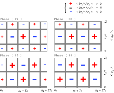
Figure 11: Schematic illustration of the phase relations among the four time-oscillating wavelike structures of the quantities $\langle\delta q_{yj}^{(n)}/p_{yj}\rangle_{t}$ as functions of the position $\langle q_{xj}\rangle_{t}$ and the collision number $n_{t}$, corresponding to the first four-point step in the same collision number interval. The spatial wavelength and the period of the time-oscillations are given by $L_{x}$ and $\mathcal{T}_{0}$, respectively. Thick gray lines means node lines, the region indicated by a red plus sign ($+$) is the region where the quantity $\langle\delta q_{yj}^{(n)}/p_{yj}\rangle_{t}$ is positive, and the region indicated by a blue minus sign ($-$) is the region where the quantity $\langle\delta q_{yj}^{(n)}/p_{yj}\rangle_{t}$ is negative. The phases [P3] and [P4] differ from the phases [P1] and [P2] by a phase shift of $\pi/2$ in the spatial direction. The phases [P1] and [P3] differ from the phases [P2] and [P4] by a phase shift of $\pi/2$ in time.

IV Quasi-One-Dimensional Systems with a Hard-wall Boundary Condition

In this section we consider quasi-one-dimensional systems with boundary conditions including a hard-wall boundary condition. Noting that there are two directions in which we have to introduce the boundary conditions, we consider the three cases of systems; [A2] the case of periodic boundary conditions in the $x$-direction and hard-wall boundary conditions in the $y$-direction, [A3] the case of hard-wall boundary conditions in the $x$-direction and periodic boundary conditions in the $y$-direction, and [A4] the case of hard-wall boundary conditions in both the directions. To adopt the hard-wall boundary condition means that there is no momentum conservation in the direction connected by hard-walls, so it allows us to discuss the role of momentum conservation in the stepwise structure of the Lyapunov spectrum by comparing models having a hard-wall boundary conditions with models having periodic boundary conditions. We will get different stepwise structures for the Lyapunov spectra in the above three cases and the case of the preceding section, and the investigation of Lyapunov vectors corresponding to steps of the Lyapunov spectra leads to relating and to categorizing them with each other.

In the systems with a hard-wall boundary condition we should carefully choose the width $L_{x}$ and the height $L_{y}$ of the systems for meaningful comparisons between the results in the systems with different boundary conditions. It should be noted that in systems with pure periodic boundary conditions, the centers of particles can reach to the periodic boundaries, while in hard-wall boundary conditions the centers of particles can only reach within a distance $R$ (the particle radius) of the hard-wall boundaries. In this sense the effective region for particles to move in the system with hard-wall boundary conditions is smaller than in the corresponding system with periodic boundary conditions, if we choose the same lengths $L_{x}$ and $L_{y}$. In this section the lengths $L_{x}$ and $L_{y}$ of the systems with a hard-wall boundary condition are chosen so that the effective region for particle to move is the same as in the pure periodic boundary case considered in the previous section, and are given by $(L_{y},L_{x})=(2R(1+10^{-6})+2R,1.5N(L_{y}-2R))$ in the case [A2], $(L_{y},L_{x})=(2R(1+10^{-6}),1.5NL_{y}+2R)$ in the case [A3] and $(L_{y},L_{x})=(2R(1+10^{-6})+2R,1.5N(L_{y}-2R)+2R)$ in the case [A4]. These choices of the lengths $L_{x}$ and $L_{y}$ also lead to the almost same mean free time in the four different boundary condition cases. In the cases of [A2] and [A4] with this choice of the system width $L_{y}$, in principle there is a space to exchange the particle positions in the $x$-direction (namely, strictly speaking these cases do not satisfy the second condition of Eq. (1) ), but the space is extremely narrow (that is $2R\times 10^{-6}$) so that it is almost impossible for particle positions to actually be exchanged.

IV.1 The case of periodic boundary conditions in the $x$-direction and hard-wall boundary conditions in the $y$-direction

The first case is the quasi-one-dimensional system with periodic boundary conditions in the $x$-direction and with hard-wall boundary conditions in the $y$-direction (the boundary case [A2]). A schematic illustration of this system is given in Fig. 12 in which periodic boundary conditions and hard-wall boundary conditions are represented as bold solid lines and broken lines, respectively.

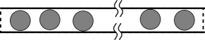
Figure 12: A schematic illustration of a quasi-one-dimensional system with periodic boundary conditions in the $x$-direction and hard-wall boundary conditions in the $y$-direction. The broken line on the boundary means to take periodic boundary conditions, and the solid line on the boundary means to take hard-wall boundary conditions.

Figure 13: Stepwise structure of the Lyapunov spectrum normalized by the maximum Lyapunov exponent for the quasi-one-dimensional system with periodic boundary conditions in the $x$-direction and hard-wall boundary conditions in the $y$-direction. Inset: Full scale of the normalized Lyapunov spectrum.

Figure 13 is the Lyapunov spectrum normalized by the maximum Lyapunov exponent $\lambda_{1}\approx 1.30$ for this system. In this figure we showed a small positive region of the Lyapunov spectrum including its stepwise structures, while the full scale of the positive branch of the Lyapunov spectrum is shown in the inset. In this system the $y$-component of the total momentum is not conserved because of the hard-wall boundary conditions in the $y$-direction, so there are only 4 zero-Lyapunov exponents in this system. This figure shows clearly that the steps of the Lyapunov spectrum consist of four-point steps only, and there is no two-point step in the Lyapunov spectrum which appears in the model discussed in the previous section. Besides, we cannot recognize a wavelike structure in the graph of Lyapunov vector components $\langle\delta q_{yj}^{(n)}\rangle$ as a function of the position $\langle q_{xj}\rangle$ (the graph [B1]) in this model. A comparison of this fact with results in the previous model suggests that the two-point step of the Lyapunov spectrum in the previous section should be strongly connected to the conservation of the $y$-component of the total momentum.

Figure 14: Local time-averaged quantities $\langle\delta q_{yj}^{(n)}/p_{yj}\rangle_{t}$ as functions of the normalized position $\langle q_{xj}\rangle_{t}/L_{x}$ and the collision number $n_{t}$ corresponding to the Lyapunov exponents $\lambda_{148}$ and $\lambda_{144}$ in the same collision number interval $[390600,396000]$. The system is the quasi-one-dimensional system with periodic boundary conditions in the $x$-direction and hard-wall boundary conditions in the $y$-direction, and the corresponding Lyapunov exponents are indicated by arrows in Fig. 13. Contour plots on the bottoms of these three-dimensional plots are given by red dotted lines, black solid lines and blue broken lines corresponding to the values $\langle\delta q_{yj}^{(n)}/p_{yj}\rangle_{t}=0.08,0$ and $-0.08$, respectively.

Figure 15: Contour plots of the time-averaged quantities $\langle\delta q_{yj}^{(n)}/p_{yj}\rangle_{t}$ as functions of the normalized position $\langle q_{xj}\rangle_{t}/L_{x}$ and the collision number $n_{t}$ corresponding to the first four-point step consisting of the Lyapunov exponents $\lambda_{n}$, $n=148,147,146$ and $145$ in the same collision number interval $[385800,396000]$. The system is the quasi-one-dimensional system with periodic boundary conditions in the $x$-direction and hard-wall boundary conditions in the $y$-direction, and the corresponding Lyapunov exponents are indicated by the brace under circles in Fig. 13. Here red dotted lines, black solid lines and blue broken lines correspond to the values $\langle\delta q_{yj}^{(n)}/p_{yj}\rangle_{t}=0.08,0$ and $-0.08$, respectively.

We consider a relation between the four-point steps in the model of this section and in the model of the previous section by investigating the graph of the quantity $\langle\delta q_{yj}^{(n)}/p_{yj}\rangle_{t}$ as a function of the normalized position $\langle q_{xj}\rangle_{t}/L_{x}$ and the collision number $n_{t}$ (the graph [B2]). Fig. 14 is such graphs, and corresponds to the Lyapunov exponent $\lambda_{148}$ in the first four-point step ( Fig. 14(a) ) and the Lyapunov exponent $\lambda_{144}$ in the second four-point step ( Fig. 14(b) ), which are indicated by arrows in Fig. 13, in the same collision number interval $[390600,396000]$. The wavelike structures of these graphs have a wavelength $1/i$ for the $i$-th four-point steps. The time-oscillating period corresponding to the Lyapunov exponent $\lambda_{148}$ is almost the same as the period $\mathcal{T}_{0}$ of the first four-point steps of the previous model, and is approximately twice as long as the time-oscillating period in the Lyapunov exponent $\lambda_{144}$ of this model. These features are common with the four-point steps in the models of the previous section, suggesting that the four-point steps of the Lyapunov spectrum in this model correspond to the four-point steps in the model of the previous section. We can also show that the quantities $\langle\delta q_{yj}^{(n)}/p_{yj}\rangle_{t}$ corresponding to the zero Lyapunov exponents $\lambda_{150}$ and $\lambda_{149}$ are constants as functions of $\langle q_{xj}\rangle_{t}$ and $n_{t}$ approximately.

Now we proceed to investigate the graph of the quantities $\langle\delta q_{yj}^{(n)}/p_{yj}\rangle_{t}$ corresponding to the Lyapunov exponents in the same four-point steps of the Lyapunov spectrum. Fig. 15 is the contour plots of these quantities as functions of the normalized position $\langle q_{xj}\rangle_{t}/L_{x}$ and the collision number $n_{t}$, corresponding to the first four-point step consisting of the Lyapunov exponents $\lambda_{n}$, $n=148,147,146$ and $145$, in the same collision number interval $[385800,396000]$. The corresponding Lyapunov exponents are indicated by the brace under circles in Fig. 13. In this case the contour lines of $\langle\delta q_{yj}^{(n)}/p_{yj}\rangle_{t}=0$ seem to be slanting, but if we pay attention of the mountain regions and the valley regions in these graphs then we can realize that the structure of these four graphs are similar to the contour plots of the four graphs in Fig. 10 for the previous model. Therefore the phase relations among the time-oscillating wavelike structures of the quantity $\langle\delta q_{yj}^{(n)}/p_{yj}\rangle_{t}$ can be summarized in the schematic illustration given in Fig. 11 like in the previous model. This suggests an approximate expression for the Lyapunov vector components given by Eq. (4), for Lyapunov vector components $\delta q_{yj}^{(n)}$ corresponding to the Lyapunov exponents of the four-point steps in this model.

IV.2 The case of hard-wall boundary conditions in the $x$-direction and periodic boundary conditions in the $y$-direction

As the next system we consider a quasi-one-dimensional system with hard-wall boundary conditions in the $x$-direction and periodic boundary conditions in the $y$-direction (the boundary case [A3]). A schematic illustration of such a system is given in Fig. 16 with solid lines for the hard-wall boundary conditions and broken lines for the periodic boundary conditions.

Figure 16: A schematic illustration of a quasi-one-dimensional system with hard-wall boundary conditions in the $x$-direction and periodic boundary conditions in the $y$-direction. The solid lines for the boundary means to take hard-wall boundary conditions, and broken lines for the boundary means to take periodic boundary conditions.

In this system the $x$-component of the total momentum is not conserved, so the total number of the zero-Lyapunov exponents is 4. Fig. 17 is a small positive region of the Lyapunov spectrum normalized by the maximum Lyapunov exponent $\lambda_{1}\approx 1.30$, including its stepwise structure, while its whole positive part of the Lyapunov spectrum is given in the inset. The stepwise structure of the Lyapunov spectrum is clearly different from the model of the previous subsection, and consists of two-point steps interrupted by isolated single Lyapunov exponents. (We call the isolated single Lyapunov exponents interrupting the two-point steps the ”one-point steps” in this paper from now on, partly because they are connected to the two-point steps in the model of Sect. III as will shown in this subsection.) As discussed in Sect. III the Lyapunov spectrum for the model with periodic boundary conditions in both directions has two-point steps and four-point steps, and it is remarkable that to adopt the hard-wall boundary conditions in the $x$-direction and to destroy the total momentum conservation in this direction halves the step-widths of both kinds of steps.

Figure 17: Stepwise structure of the Lyapunov spectrum normalized by the maximum Lyapunov exponent for the quasi-one-dimensional system with hard-wall boundary conditions in the $x$-direction and periodic boundary conditions in the $y$-direction. Inset: Full scale of the normalized Lyapunov spectrum. The circle dots filled by black (gray) are the Lyapunov exponents accompanying wavelike structure (a constant behavior) of the Lyapunov vector components $\langle\delta q_{yj}^{(n)}\rangle$ partly shown in Fig. 18.

Fig. 18 is the graphs of the time-averaged Lyapunov vector components $\langle\delta q_{yj}^{(n)}\rangle$ as functions of the normalized position $\langle q_{xj}\rangle/L_{x}$ (the graph [B1]), corresponding to the one-point steps. We can clearly recognize wavelike structures in these graphs, and in this sense the one-point steps in this model should be strongly related to the two-point steps in the model of Sect. III. The Lyapunov exponents accompanying wavelike structure of this kind of graphs are shown in Fig. 17 as black-filled circle dots, meaning that they are the one-point steps. In Fig. 17 we also filled the circle dots by gray for one of the zero-Lyapunov exponents in which the graph of the Lyapunov vector components $\langle\delta q_{yj}^{(n)}\rangle$ as a function of the position $\langle q_{xj}\rangle$ is constant approximately. However it is important to note that the wavelength of the wave corresponding to the $i$-th one-point step in this model is $2/i$, not $1/i$ like in the model of Sect. III. We fitted the graphs corresponding to the Lyapunov exponents $\lambda_{n}$, $n=149,148,145$ and $142$ by the functions $y=\alpha_{149},\alpha_{148}\cos(\pi x+\beta_{148}),\alpha_{145}\cos(2\pi x+\beta_{145}),\alpha_{142}\cos(3\pi x+\beta_{142})$ respectively, with $\alpha_{n}$ and $\beta_{n}$ as fitting parameters. Here the values of the fitting parameters are chosen as $\alpha_{149}=0.11547$, $(\alpha_{148},\beta_{148})=(0.16213,-0.0089778)$, $(\alpha_{145},\beta_{145})=(-0.16202,-0.01007)$ and $(\alpha_{142},\beta_{142}=(-0.15945,0.0089148)$. The graphs are very nicely fitted by a constant or the sinusoidal functions, and lead to the form

$$\delta q_{yj}^{(n(k))}\approx\alpha_{k}^{\prime}\cos\left(\frac{\pi k}{L_{x}}q_{xj}+\beta_{k}^{\prime}\right),$$ (5)

$j=1,2,\cdots,N$, of the Lyapunov vector component $\delta q_{yj}^{(n(k))}$ corresponding to the Lyapunov exponents $\lambda_{n(k)}$ in the $k$-th one-point step with constants $\alpha_{k}^{\prime}$ and $\beta_{k}^{\prime}$.

Figure 18: Time-averaged Lyapunov vector components $\langle\delta q_{yj}^{(n)}\rangle$ corresponding to the $n$-th Lyapunov exponent $\lambda_{n}$, $n=149,148,145$ and $142$, as functions of the time-averaged particle position $\langle q_{xj}\rangle/L_{x}$ normalized by the system length $L_{x}$. The system is the quasi-one-dimensional system with hard-wall boundary conditions in the $x$-direction and periodic boundary conditions in the $y$-direction, and the corresponding Lyapunov exponents are shown as the black- and gray-filled circles in Fig. 17. The numerical data are fitted by a constant and sinusoidal functions.

Now we investigate the remaining steps, namely the two-point steps of the Lyapunov spectrum. Corresponding to these two-point steps of the Lyapunov spectrum, the graphs of the quantity $\langle\delta q_{yj}^{(n)}/p_{yj}\rangle_{t}$ as functions of the normalized position $\langle q_{xj}\rangle_{t}/L_{x}$ and the collision number $n_{t}$ (the graph [B2]) show spatial wavelike structures oscillating in time. It is shown in Fig. 19 for those graphs corresponding to Lyapunov exponents (indicated by arrows in Fig. 17) in different two-point step, in the same collision number interval $[222000,232200]$. The spatial wavelength of the waves corresponding to the $i$-th two-point step is $2/i$, which is twice as long as the wavelength of waves of the four-point steps in the models in Sect. III and the previous subsection. The period of time-oscillation of the wave corresponding to the $i$-th two-point step of the Lyapunov spectrum is approximately given by $\mathcal{T}_{0}^{\prime}/i$ with a constant $\mathcal{T}_{0}^{\prime}$. This kind of graph corresponding to one of the zero-Lyapunov exponents, namely $\lambda_{150}$, is almost constant.

Figure 19: Local time-averaged quantities $\langle\delta q_{yj}^{(n)}/p_{yj}\rangle_{t}$ as functions of the normalized position $\langle q_{xj}\rangle_{t}/L_{x}$ and the collision number $n_{t}$ corresponding to the Lyapunov exponents $\lambda_{n}$, $n=147,144$ and $141$ in the same collision number interval $[222000,232200]$. The system is the quasi-one-dimensional system with hard-wall boundary conditions in the $x$-direction and periodic boundary conditions in the $y$-direction, and the corresponding Lyapunov exponents are indicated by arrows in Fig. 17. Contour plots on the bottoms of these three-dimensional plots are given by red dotted lines, black solid lines and blue broken lines corresponding to the values $\langle\delta q_{yj}^{(n)}/p_{yj}\rangle_{t}=0.08,0$ and $-0.08$, respectively.

It is important to note a relation between the time-oscillating period $\mathcal{T}_{0}$ of the preceding two models and the time-oscillating period $\mathcal{T}_{0}^{\prime}$ of the model in this section. Noting that in Figs. 9(a), 14(a) and 19(a) we plotted about one period of the time-oscillation of the wavelike structures of the quantities $\langle\delta q_{yj}^{(n)}/p_{yj}\rangle_{t}$ in the collision time intervals [543000,548100], [390600,396000] and [222000,232200], respectively, we can get an approximate relation $\mathcal{T}_{0}^{\prime}\approx 2\mathcal{T}_{0}$.

Figure 20: Contour plots of the local time-averaged quantities $\langle\delta q_{yj}^{(n)}/p_{yj}\rangle_{t}$ as functions of the normalized position $\langle q_{xj}\rangle_{t}/L_{x}$ and the collision number $n_{t}$ corresponding to the first two-point step consisting of the Lyapunov exponents $\lambda_{n}$, $n=147$ and $146$ in the same collision number interval $[212400,232200]$. The system is the quasi-one-dimensional system with hard-wall boundary conditions in the $x$-direction and periodic boundary conditions in the $y$-direction, and the corresponding Lyapunov exponents are indicated by the brace under circles in Fig. 17. Here red dotted lines, black solid lines and blue broken lines correspond to the values $\langle\delta q_{yj}^{(n)}/p_{yj}\rangle_{t}=0.08,0$ and $-0.08$, respectively.

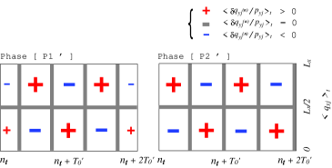
Figure 21: Schematic illustration of the phase relations among the time-oscillating wavelike structures of the quantities $\langle\delta q_{yj}^{(n)}/p_{yj}\rangle_{t}$ as functions of the position $\langle q_{xj}\rangle_{t}$ and the collision number $n_{t}$, corresponding to the first two-point step in the same collision number interval. Thick gray lines means node lines, the region indicated by a red plus sign ($+$) is the region where the quantity $\langle\delta q_{yj}^{(n)}/p_{yj}\rangle_{t}$ is positive, and the region indicated by a blue minus sign ($-$) is the region where the quantity $\langle\delta q_{yj}^{(n)}/p_{yj}\rangle_{t}$ is negative. The phase of [P1’] is shifted in time from the phase of [P2’] by $\pi/2$.

The next problem is to investigate the graphs of the quantities $\langle\delta q_{yj}^{(n)}/p_{yj}\rangle_{t}$ as a function of the position $\langle q_{xj}\rangle_{t}$ and the collision number $n_{t}$ in the same two-point step of the Lyapunov spectrum. Fig. 20 is the contour plots of such graphs for the first two-point step consisting of the Lyapunov exponents $\lambda_{n}$, $n=147$ and $146$, which is indicated by a brace under circles in Fig. 17, in the same collision number interval $[212400,232200]$. It should be noted that the positions of the nodes of two spatial waves belonging to the same two-point step almost coincide with each other. However the phases of the time-oscillations of the amplitudes of the waves are shifted by about $\pi/2$ with each other. The phase relations of the graphs 20(a) and (b) is visualized in the schematic illustration given in Fig. 21 of the time-oscillating wavelike structures of the quantities $\langle\delta q_{yj}^{(n)}/p_{yj}\rangle_{t}$ corresponding to the first two-point step in the same collision number interval. Here the phase [P1’] and [P2’] correspond to Figs. 20(a) and (b), respectively. A similar investigation of the Lyapunov vectors shows that the time-oscillating wavelike structures for the second two-point steps are like the phases [P1] and [P2] of Fig. 11 except that the period $\mathcal{T}_{0}$ in Fig. 11 should be replaced with the oscillating period $\mathcal{T}_{0}^{\prime}$ of this model. These results suggest that the two-point steps in this model correspond to the four-point steps in the models of the previous subsection and Sect. III, except for differences in the values of their wavelengths and time-oscillating periods. After all we get a conjecture that the Lyapunov vector components $\delta q_{yj}^{(\tilde{n}(k))}$ and $\delta q_{yj}^{(\tilde{n}(k)-1)}$ corresponding to the Lyapunov exponents constructing the $k$-th two-point step are approximately expressed as

$$\left\{\delta q_{yj}^{(\tilde{n}(k))},\;\delta q_{yj}^{(\tilde{n}(k)-1)}\right\}\approx$$

$$\left\{\tilde{\alpha}_{k}^{\prime}\;p_{yj}\cos\left(\frac{\pi k}{L_{x}}q_{xj}\!+\!\tilde{\beta}_{k}^{\prime}\right)\cos\left(\frac{\pi k}{\mathcal{T}_{0}}n_{t}\!+\!\tilde{\gamma}_{k}^{\prime}\right),\right.$$

$$\left.\tilde{\alpha}_{k}^{\prime}\;p_{yj}\cos\left(\frac{\pi k}{L_{x}}q_{xj}\!+\!\tilde{\beta}_{k}^{\prime}\right)\sin\left(\frac{\pi k}{\mathcal{T}_{0}}n_{t}\!+\!\tilde{\gamma}_{k}^{\prime}\right)\right\},$$ (6)

$j=1,2,\cdots,N$ with constants $\tilde{\alpha}_{k}^{\prime}$, $\tilde{\beta}_{k}^{\prime}$ and $\tilde{\gamma}_{k}^{\prime}$, noting the time-oscillating period $\mathcal{T}_{0}^{\prime}\approx 2\mathcal{T}_{0}$.

IV.3 The case of hard-wall boundary conditions in both directions

The last model is the case of hard-wall boundary conditions in both directions (the boundary case [A4]). A schematic illustration of this system is given in Fig. 22 in which the solid line of the boundary means to take hard-wall boundary conditions.

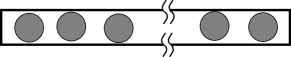
Figure 22: A schematic illustration of a quasi-one-dimensional system with hard-wall boundary conditions in both directions. The solid line of the boundary means to take the hard-wall boundary conditions.

A small positive region of the Lyapunov spectrum normalized by the maximum Lyapunov exponent $\lambda_{1}\approx 1.28$ is given in Fig. 23. The graph for the full scale of the positive branch of the normalized Lyapunov spectrum is also given in the inset of this figure. In this system the total momentum is not conserved any more, and the total number of zero-Lyapunov exponents is 2. The stepwise structure of the Lyapunov spectrum consists of two-point steps only. In this model a wavelike structure in the Lyapunov vector component $\langle\delta q_{yj}^{(n)}\rangle$ as a function of the position $\langle q_{xj}\rangle$ (the graph [B1]) is not observed.

Figure 23: Stepwise structure of the Lyapunov spectrum normalized by the maximum Lyapunov exponent for a quasi-one-dimensional system with hard-wall boundary conditions in both directions. Inset: Full scale of the normalized Lyapunov spectrum.

Fig. 24 is the graphs of the quantities $\langle\delta q_{yj}^{(n)}/p_{yj}\rangle_{t}$ as functions of the normalized position $\langle q_{xj}\rangle_{t}/L_{x}$ and the collision number $n_{t}$ (the graph [B2]), corresponding to the Lyapunov exponents $\lambda_{n}$, $n=149,147$ and $145$, in the same collision number interval $[235200,246000]$. The corresponding Lyapunov exponents are indicated by arrows in Fig. 23. This figure for the two-point steps of the Lyapunov spectrum shows a similar wavelike structure to the wavelike structure of the quantities $\langle\delta q_{yj}^{(n)}/p_{yj}\rangle_{t}$ in the model of the previous subsection, although one may think that fluctuations of these graphs in this model are much smaller than in the previous model. This suggest that the two-point steps of the Lyapunov spectrum in Fig. 23 are similar to the two-point steps in the model of the previous subsection. The wavelength of the spatial waves and the the periods of the time-oscillations corresponding to the $i$-th two-point step are $2/i$ and $\mathcal{T}_{0}^{\prime}/i$, respectively, and the time-oscillating period of the first two-point step is given approximately by the same period $\mathcal{T}_{0}^{\prime}$ $(\approx 2\mathcal{T}_{0})$ as in the model of the previous subsection. It may also be noted that this kind of graph corresponding to the zero-Lyapunov exponent $\lambda_{150}$ is almost constant.

Figure 24: Local time-averaged quantities $\langle\delta q_{yj}^{(n)}/p_{yj}\rangle_{t}$ as functions of the normalized position $\langle q_{xj}\rangle_{t}/L_{x}$ and the collision number $n_{t}$ corresponding to the Lyapunov exponents $\lambda_{n}$, $n=149,147$ and $145$ in the same collision number interval $[235200,246000]$. The system is the quasi-one-dimensional system with hard-wall boundary conditions in both directions, and the corresponding Lyapunov exponents are indicated by arrows in Fig. 23. Contour plots on the bottoms of these three-dimensional plots are given by red dotted lines, black solid lines and blue broken lines corresponding to the values $\langle\delta q_{yj}^{(n)}/p_{yj}\rangle_{t}=0.08,0$ and $-0.08$, respectively.

Fig. 25 is the contour plots of the quantities $\langle\delta q_{yj}^{(n)}/p_{yj}\rangle_{t}$ as functions of the normalized position $\langle q_{xj}\rangle_{t}/L_{x}$ and the collision number $n_{t}$ corresponding to the Lyapunov exponents $\lambda_{n}$, $n=149$ and $148$ in the first two-point step of the Lyapunov spectrum in the same collision number interval $[223800,246000]$. The corresponding Lyapunov exponents are indicated by the brace under circles in Fig. 23. Similarly to the previous model, the nodes of two spatial waves corresponding to the same two-point step almost coincide with each other, and the phase of the time-oscillation of the wave amplitudes is shifted by about $\pi/2$. This also says that the phase relations of the graphs 25(a) and (b) is the types of the phases [P1’] and [P2’] in Fig. 21. In a similar way we can see that the time-oscillating wavelike structures for the second two-point steps of the Lyapunov spectrum for this model are like the phases [P1] and [P2] of Fig. 11 by replacing the period $\mathcal{T}_{0}$ of Fig. 11 with the time-oscillating period $\mathcal{T}_{0}^{\prime}\approx 2\mathcal{T}_{0}$ of this model. These suggest an approximate expression for the Lyapunov vector components given by Eq. (6), for Lyapunov vector components $\delta q_{yj}^{(n)}$ corresponding to the Lyapunov exponents of the $k$-th two-point steps in this model. The fact that the only difference between the model in this subsection and the model in the previous subsection is the boundary conditions in the $y$-direction suggests that the one-point steps of the model in the previous subsection come from the conservation of the $y$-component of the total momentum.

Figure 25: Contour plots of the local time-averaged quantities $\langle\delta q_{yj}^{(n)}/p_{yj}\rangle_{t}$ as functions of the normalized position $\langle q_{xj}\rangle_{t}/L_{x}$ and the collision number $n_{t}$ corresponding to the first two-point step consisting of the Lyapunov exponents $\lambda_{n}$, $n=149$ and $148$ in the same collision number interval $[223800,246000]$. The system is the quasi-one-dimensional system with hard-wall boundary conditions in both directions, and the corresponding Lyapunov exponents are indicated by the brace under circles in Fig. 23. Here, red dotted lines, black solid lines and blue broken lines correspond to the values $\langle\delta q_{yj}^{(n)}/p_{yj}\rangle_{t}=0.08,0$ and $-0.08$, respectively.

Table 1: The stepwise structures of the Lyapunov spectra and the associated wavelike structures of the Lyapunov vectors in the four boundary cases considered in this paper. The boundary cases [A1], [A2], [A3] and [A4] were considered in the sections III, IV.1, IV.2 and IV.3, respectively. In this table, $\mathcal{S}$ is the number of points in the step (or the number of the zero Lyapunov exponents in the line specified by the label ”$\lambda_{n}=0$”), $\mathcal{L}$ is the wavelength of spatial wavelike structure, and $\mathcal{T}$ is the period of time-oscillation of the wave, $L_{x}$ is the length of the quasi-one-dimensional rectangle, and $\mathcal{T}_{0}$ is constant.

Boundary case [A1]

Boundary case [A2]

Boundary case [A3]

Boundary case [A4]

mode

$\mathcal{S}$

$\mathcal{L}$

$\mathcal{T}$

$\mathcal{S}$

$\mathcal{L}$

$\mathcal{T}$

$\mathcal{S}$

$\mathcal{L}$

$\mathcal{T}$

$\mathcal{S}$

$\mathcal{L}$

$\mathcal{T}$

$\lambda_{n}=0$

6

-

-

4

-

-

4

-

-

2

-

-

$\delta q_{yj}^{(n)}$

2

$L_{x}$/1

-

-

-

-

1

2$L_{x}$/1

-

-

-

-

$\delta q_{yj}^{(n)}/p_{yj}$

4

$L_{x}$/1

$\mathcal{T}_{0}$/1

4

$L_{x}$/1

$\mathcal{T}_{0}$/1

2

2$L_{x}$/1

$2\mathcal{T}_{0}$/1

2

2$L_{x}$/1

$2\mathcal{T}_{0}$/1

$\delta q_{yj}^{(n)}$

2

$L_{x}$/2

-

-

-

-

1

2$L_{x}$/2

-

-

-

-

$\delta q_{yj}^{(n)}/p_{yj}$

4

$L_{x}$/2

$\mathcal{T}_{0}$/2

4

$L_{x}$/2

$\mathcal{T}_{0}$/2

2

2$L_{x}$/2

$2\mathcal{T}_{0}$/2

2

2$L_{x}$/2

$2\mathcal{T}_{0}$/2

$\delta q_{yj}^{(n)}$

$\vdots$

$\vdots$

$\vdots$

$\vdots$

$\vdots$

$\vdots$

1

2$L_{x}$/3

-

-

-

-

$\delta q_{yj}^{(n)}/p_{yj}$

$\vdots$

$\vdots$

$\vdots$

$\vdots$

$\vdots$

$\vdots$

2

2$L_{x}$/3

$2\mathcal{T}_{0}$/3

2

2$L_{x}$/3

$2\mathcal{T}_{0}$/3

$\vdots$

$\vdots$

$\vdots$

$\vdots$

$\vdots$

$\vdots$

$\vdots$

$\vdots$

$\vdots$

$\vdots$

$\vdots$

$\vdots$

$\vdots$

V Conclusion and Remarks

In this paper we have discussed numerically the stepwise structure of the Lyapunov spectra and its corresponding wavelike structures for the Lyapunov vectors in many-hard-disk systems. We concentrated on the quasi-one-dimensional system whose shape is a very narrow rectangle that does not allow exchange of disk positions. In the quasi-one-dimensional system we can get a stepwise structure of the Lyapunov spectrum in a relatively small system, for example, even in a 10-particle system, whereas a fully two-dimensional system would require a much more particles. In such a system we have considered the following two problems: [A] How does the stepwise structure of the Lyapunov spectra depend on boundary conditions such as periodic boundary conditions and hard-wall boundary conditions? [B] How can we categorize the stepwise structure of the Lyapunov spectra using the wavelike structure of the corresponding Lyapunov vectors? To consider the problem [A] also means to investigate the effects of the total momentum conservation law on the stepwise structure of the Lyapunov spectra. In this paper we considered four types of the boundary conditions; [A1] periodic boundary conditions in the $x$- and $y$-directions, [A2] periodic boundary conditions in the $x$-direction and hard-wall boundary conditions in the $y$-direction, [A3] hard-wall boundary conditions in the $x$-direction and periodic boundary conditions in the $y$-direction, and [A4] hard-wall boundary conditions in the $x$- and $y$-directions, in which we took the $y$-direction as the narrow direction of the rectangular shape of the system. With each boundary case we obtained different stepwise structures of the Lyapunov spectra. In each boundary condition we also considered graphs of the following two quantities; [B1] the $y$-component $\delta q_{yj}^{(n)}$ of the spatial coordinate part of the Lyapunov vector of the $j$-th particle corresponding to the Lyapunov exponent $\lambda_{n}$ as a function of the $x$-component $q_{xj}$ of the spatial component of the $j$-th particle, and [B2] the quantity $\delta q_{yj}^{(n)}/p_{yj}$ with the $y$-component $p_{yj}$ of the momentum coordinate of the $j$-th particle as a function of the position $q_{xj}$ and the collision number $n_{t}$. These quantities $\delta q_{yj}^{(n)}$ and $\delta q_{yj}^{(n)}/p_{yj}$ give constant values in some of zero-Lyapunov exponents, at least approximately. We found that the steps of the Lyapunov spectra accompany a wavelike structure in the quantity $\delta q_{yj}^{(n)}$ or $\delta q_{yj}^{(n)}/p_{yj}$, depending on the kind of steps of the Lyapunov spectra. A time-dependent oscillating behavior appears in the wavelike structure of the quantity $\delta q_{yj}^{(n)}/p_{yj}$, whereas the wavelike structure of the quantity $\delta q_{yj}^{(n)}$ is essentially stationary. Fluctuations of these quantities $\delta q_{yj}^{(n)}$ and $\delta q_{yj}^{(n)}/p_{yj}$ disturb their clear oscillatory structures, so we took a time-average of these quantities (a local time-average for the quantity $\delta q_{yj}^{(n)}/p_{yj}$ because of its time-oscillating behavior, and a longer time-average for the quantity $\delta q_{yj}^{(n)}$ because it is much more stationary in time than the quantity $\delta q_{yj}^{(n)}/p_{yj}$) to get their dominant wavelike structures. In Table. 1 we summarize our results about the characteristics of the stepwise structures of the Lyapunov spectra and the wavelike structures of the Lyapunov vectors in the four boundary cases [A1], [A2], [A3] and [A4]. In Lyapunov exponents in each step of the Lyapunov spectra the wavelike structures of the quantity $\delta q_{yj}^{(n)}$ or $\delta q_{yj}^{(n)}/p_{yj}$ are approximately orthogonal to each others in space (in the sense of Eq. (3)), in space and time (in the sense of Eq. (4)) or in time (in the sense of Eq. (6)), and this fact suggests that the wavelike structure of these quantities are sufficient to categorize the stepwise structure of the Lyapunov spectra in the quasi-one-dimensional systems considered in this paper.

Different from a purely two-dimensional model such as a square system in which each particle can collide with any other particle, in the quasi-one-dimensional model a separation between the stepwise region and the smoothly changing region of the Lyapunov spectrum is not clear. In Ref. Tan02 this point was explained as being caused by the fact that particles interact only with the two nearest-neighbor particles, whereas in the purely two-dimensional low-density system particles can interact with more than two particles.

In this paper we considered the quasi-one-dimensional systems only. However there should be many interesting other situations in which we can investigate structures of the Lyapunov spectrum and the Lyapunov vectors. For example, we may investigate the effect of the rotational invariance of the system on such structures by considering a two-dimensional system with a circle shape. One might also investigate the system in which the orbit is not deterministic any more, in order to know whether the deterministic orbit plays an important role in the stepwise structure of the Lyapunov spectrum or not. It may also be important to investigate the dependence of the stepwise structures of the Lyapunov spectra on the spatial dimension of the system, for example, to investigate any structure of the Lyapunov spectra for purely one- or three-dimensional many particle systems. (Note that the quasi-one-dimensional systems considered in this paper are still two-dimensional systems in the sense of the phase space dimension.) These problems remain to be investigated in the future.

References

- (1) P. Gaspard, Chaos, scattering and statistical mechanics (Cambridge University press, 1998).
- (2) J. R. Dorfman, An introduction to chaos in nonequilibrium statistical mechanics (Cambridge University press, 1999).
- (3) Ch. Dellago, H. A. Posch, and W. G. Hoover, Phys. Rev. E 53, 1485 (1996).
- (4) Lj. Milanović, H. A. Posch, and Wm. G. Hoover, Mol. Phys. 95, 281 (1998).
- (5) H. A. Posch and R. Hirschl, in Hard ball systems and the Lorentz gas, edited by D. Szász (Springer, Berlin, 2000), p. 279.
- (6) S. McNamara and M. Mareschal, Phys. Rev. E 63, 061306 (2001).
- (7) H. A. Posch and Ch. Forster, in Lecture Notes on Computer Science, edited by P. M. A. Sloot et al. (Springer-Verlag, Berlin, 2002), p. 1170.
- (8) K. Kaneko, Physica 23 D, 436 (1986).
- (9) K. Ikeda and K. Matsumoto, J. Stat. Phys. 44, 955 (1986).
- (10) I. Goldhirsch, P. -L. Sulem, and S. A. Orszag, Physica 27D, 311 (1987).
- (11) M. Falcioni, U. M. B. Marconi, and A. Vulpiani, Phys. Rev. A 44, 2263 (1991).
- (12) T. Konishi and K. Kaneko, J. Phys. A: Math. Gen. 25, 6283 (1992).
- (13) M. Yamada and K. Ohkitani, Phys. Rev. E 57, R6257 (1998).
- (14) A. Pikovsky and A. Politi, Phys. Rev. E 63, 036207 (2001).
- (15) Y. Y. Yamaguchi and T. Iwai, Phys. Rev. E 64, 066206 (2001).
- (16) T. Taniguchi, C. P. Dettmann, and G. P. Morriss, J. Stat. Phys. 109, 747 (2002).
- (17) T. Taniguchi and G. P. Morriss, Phys. Rev. E 65, 056202 (2002).
- (18) J. -P. Eckmann and O. Gat, J. Stat. Phys. 98, 775 (2000).
- (19) S. McNamara and M. Mareschal, Phys. Rev. E 64, 051103 (2001).
- (20) A. de Wijn and H. van Beijeren, in International Workshop and Seminar on Microscopic Chaos and Transport in Many-Particle Systems (Max-Planck-Institut für Physik komplexer Systeme, Dresden, Germany, 2002), (unpublished).
- (21) Ch. Forster and H. A. Posch, in International Workshop and Seminar on Microscopic Chaos and Transport in Many-Particle Systems (Max-Planck-Institut für Physik komplexer Systeme, Dresden, Germany, 2002), (unpublished).
- (22) V. I. Arnold, Mathematical methods of classical mechanics, 2nd ed. (Springer-Verlag, 1989).
- (23) G. Benettin, L. Galgani, and J. -M. Strelcyn, Phys. Rev. A 14, 2338 (1976).
- (24) I. Shimada and T. Nagashima, Prog. Theor. Phys. 61, 1605 (1979).
- (25) H. van Beijeren, A. Latz, and J. R. Dorfman, Phys. Rev. E 57, 4077 (1998).