QUASI-INTEGRABILITY IN A CLASS OF SYSTEMS

GENERALIZING THE PROBLEM OF TWO FIXED CENTERS

A. ALBOUY

IMCCE

77, av. Denfert-Rochereau, 75014 Paris, France

albouy@bdl.fr

T.J. STUCHI

Instituto de Física, Universidade Federal do Rio de Janeiro

Caixa Postal 68528

21941-972, Rio de Janeiro, Brazil

tstuchi@if.ufrj.br

Abstract. The problem of two fixed centers is a classical integrable problem, stated and integrated by Euler in 1760. The integrability is due to the unexpected first integral $G$. Some straightforward generalizations of the problem still have the generalization of $G$ as a first integral, but do not possess the energy integral. We present some numerical integrations suggesting that in the domain of bounded orbits the behavior of these a priori non hamiltonian systems is very similar to the behavior of usual quasi-integrable systems.

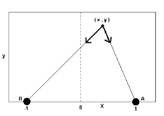
Figure 1: In Euler problem as well as in the generalizations we present, a particle at the position $(x,y)$ evolves under the action of two centers A and B, with respective coordinates $(1,0)$ and $(-1,0)$.

The equations. Euler’s problem in the plane (see Figure 1) is defined by the system of differential equations

$$\ddot{x}=-a(x_{A},y)x_{A}-b(x_{B},y)x_{B},\quad\ddot{y}=-a(x_{A},y)y-b(x_{B},y)y.$$

The two fixed centers are the points $(1,0)$ and $(-1,0)$, and the moving particle is the point $(x,y)$. We have set $x_{A}=x-1$, $x_{B}=x+1$,

$$a(\xi,\eta)=m_{A}(\xi^{2}+\eta^{2})^{-3/2},\qquad b(\xi,\eta)=m_{B}(\xi^{2}+\eta^{2})^{-3/2}.$$

The problem can be defined in the 3-dimensional space in the same way, and is also integrable, as was noticed by Euler. However, we will restrict ourselves to the planar case.

The first step in Euler’s integration was to exhibit two independent first integrals of the motion. One is the energy

$$H=(\dot{x}^{2}+\dot{y}^{2})/2-\tilde{a}(x_{A},y)-\tilde{b}(x_{B},y),$$

with $\tilde{a}(\xi,\eta)=m_{A}(\xi^{2}+\eta^{2})^{-1/2}$, $\tilde{b}(\xi,\eta)=m_{B}(\xi^{2}+\eta^{2})^{-1/2}$. We will call the second one Euler’s integral:

$$G=C_{A}C_{B}-2\tilde{a}(x_{A},y)x_{A}+2\tilde{b}(x_{B},y)x_{B},$$

with $C_{A}=x_{A}\dot{y}-y\dot{x}$, $C_{B}=x_{B}\dot{y}-y\dot{x}$. Euler continued the integration, eliminating the second derivatives in (1) using the first integrals, and separating the variables.

Our generalization is simply to consider system (1) in the case where $a$ and $b$ are any homogeneous functions of degree $-3$. Indeed, we want to put a little restriction on these homogeneous functions. We will suppose that both differential forms $\xi a(\xi,\eta)(\xi d\eta-\eta d\xi)$ and $\eta a(\xi,\eta)(\xi d\eta-\eta d\xi)$ are exact forms on the plane minus the origin, and that the same is true when we change $a$ in $b$. This hypothesis comes from the study of the problem of one fixed center (see [2] and [3]). It is not a strong restriction: the forms are already closed, so the condition on each function is just the cancellation of two scalar quantities, namely the integrals of both forms on a closed path around the origin.

It can be shown that any function $a(\xi,\eta)$ satisfying the above conditions comes from a function $A(\xi,\eta)$ homogeneous of degree $1$ as follows. Let us denote by $A_{\xi}$, $A_{\eta}$ the first derivatives of the function $A$ and by $A_{\xi\xi}$, $A_{\xi\eta}$, $A_{\eta\eta}$ the second derivatives. Then

$$a(\xi,\eta)=\eta^{-2}A_{\xi\xi}=-\xi^{-1}\eta^{-1}A_{\xi\eta}=\xi^{-2}A_{\eta\eta}.$$

The function $a(\xi,\eta)$ in Euler’s case $(2)$ is obtained in this way from the function $A=m_{A}(\xi^{2}+\eta^{2})^{1/2}$. We also have $A_{\xi}=\xi\tilde{a}$. It was discovered by the first author that $G$ persists in the form

$$G=C_{A}C_{B}-2A_{\xi}(x_{A},y)+2B_{\xi}(x_{B},y),$$

where $B(\xi,\eta)$ and $B_{\xi}(\xi,\eta)$ are associated to the function $b$ in the same way as $A$ and $A_{\xi}$ are associated to $a$. In general, no integral takes the place of the energy integral.

Quasi-integrability. We report our numerical exploration of these generalized Euler’s problems, showing three examples that seem to us significant. In all cases we met, the result is either escape or quasi-integrable behavior. The third experiment displays some islands suggesting non integrability. Magnifying the neighborhood of a saddle point, a domain of irregular dynamics can be observed.

The obvious choice for a Poincaré section is to fix the integral $G$ and take, for example, $y=0$ $(\dot{y}>0)$. In each case, we show the iterates of some points of this Poincaré mapping, the central orbit in the section and some typical quasiperiodic orbit. All the orbits in a given field of forces have the same value of Euler’s integral. Since the examples have very large orbits, we have taken throughout the numerical experiments a somewhat arbitrary cut-off criterion given by the value of any coordinate or velocity greater than a thousand. In all the examples, we have taken $A(\xi,\eta)=(5\xi^{2}-\xi\eta+5\eta^{2})/10r$, where $r=\sqrt{\xi^{2}+\eta^{2}}$, which corresponds to $a(\xi,\eta)=(5\xi^{2}+3\xi\eta+5\eta^{2})/10r$.

First example. Figures 2 to 4 correspond to $B(\xi,\eta)=-(\xi^{3}-3\xi\eta^{2})/4r^{2}+r$, and thus $b(\xi,\eta)=-2(3\xi\eta^{2}-\xi^{3})/r^{6}+r^{-3}$. The Poincaré map is close to a linear map, on a whole domain delimited by the escape criterion. This is quite strange. An explanation for this phenomena comes from geometrical considerations. We have chosen the plane as the domain for the motion, but there is a natural bigger domain for this kind of systems. It is the manifold of half lines drawn from the origin in a $3-$dimensional vector space. Our plane is from this point of view just one half of the natural domain, a hemisphere chosen arbitrarily. Escaping orbits appear as orbits cut by the boundary of the hemisphere (in the classical Kepler problem, hyperbolas appear in the same way as cut ellipses). The theoretical grounds for this remark may be found in [4].

Second example. In Figures 5 to 7, we have chosen $B=4(\xi^{4}+\eta^{4})^{1/4}$, $b=12\xi^{2}\eta^{2}(\xi^{4}+\eta^{4})^{-7/4}$. Here the section displays a wide domain with strong torsion but we are still very close from an integrable system. This rises the question: what are the integrable systems nearby? We know very few cases where our generalized Euler problem is integrable, namely the classical case and its projective transformations defined in [4] (which correspond for example to replace $\xi^{2}+\eta^{2}$ in Eq. (2) for $b$ by any homogeneous quadratic expression in $\xi$, $\eta$, and leave $a$ as it is.) Because we needed to get sufficiently many bounded orbits we were probably forced to stay close from integrable cases.

Third example and final comments. In Figures 8 to 11, we have chosen $B=(3\xi^{2}-\xi\eta+3\eta^{2})/3r$, $b=(\xi^{2}+\xi\eta+\eta^{2})/r^{5}$. Here the system behaves as a typical conservative system close to an integrable system. We are more accustomed to observe this in the class of hamiltonian systems, and one can argue that maybe the system is hamiltonian for some symplectic form. We do not believe so, and rather relate this quasi-integrability to KAM theory applied to reversible systems (see [5], Theorem 2.9). Our systems are clearly reversible.

Acknowledgments. We thank Prof. H. Cabral and the Departamento de Matemática da Universidade Federal de Pernambuco for their hospitality, Prof. A. Neishtadt for stimulating comments, and Prof. Carles Simó for his rk78 code and his very useful comments.

References

[1] L. Euler, De motu corporis ad duo centra virium fixa attracti, Problème. Un corps étant attiré en raison réciproque quarrée des distances vers deux points fixes donnés trouver les cas où la courbe décrite par ce corps sera algébrique. Opera Omnia, S. 2, vol 6. (1764, 1765, 1760) pp. 209–246, 247–273, 274–293

[2] A. Albouy, Lectures on the two-body problem, Classical and Celestial Mechanics: The Recife Lectures, H. Cabral F. Diacu editors, volume “in press”, Princeton University Press

[3] G. Darboux, Sur une loi particulière de la force signalée par Jacobi, Note 11 au cours de mécanique de Despeyrous, tome premier, A. Hermann, Paris (1884)

[4] P. Appell, Sur les lois de forces centrales faisant décrire à leur point d’application une conique quelles que soient les conditions initiales, American Journal of Mathematics 13 (1891) pp. 153–158

[5] J. Moser, Stable and Random Motions in Dynamical Systems, With Special Emphasis on Celestial Mechanics, Princeton University Press (1973)

Figure 2: Example 1; $B=-(\xi^{3}-3\xi\eta^{2})/4r^{2}+r$; $G=5.50433086$. Poincaré section $(y=0,\dot{y}>0)$, from the central periodic orbit to the neighborhood of the last torus before cut-off.

Figure 3: Example 1 again. Configuration space of the periodic orbit: $x=2.352375$, $\dot{x}=0.3621675$ and $\dot{y}=1.050626$.

Figure 4: Example 1. The configuration space of the last orbit shown in the Poincaré section just before our escape criterion is satisfied: $x=3.469875$, $\dot{x}=0.3621675$ and $\dot{y}=0.99058834$.

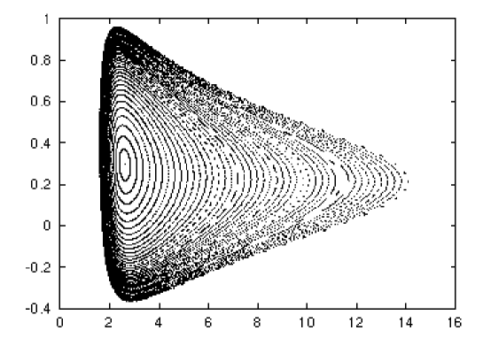
Figure 5: Example 2; $B=-(\xi^{3}-3\xi\eta^{2})/4r^{2}+r$; $G=10.9200094$. Same Poincaré section as Figure 2, showing again a phase space foliated by invariant tori up to the escape orbit.

Figure 6: Example 2. The configuration space of the periodic orbit with initial conditions $x=2.6$, $\dot{x}=0.2934$ and $\dot{y}=0.8249589$.

Figure 7: Example 2. Top: A typical torus at $x=6.1$, $\dot{x}=0.2934$ and $\dot{y}=0.3290253$; Bottom: A detail of the last torus before escape with initial conditions $x=13.6$, $\dot{x}=0.2934$ and $\dot{y}=0.145976133$.

Figure 8: Example 3; $B=(3\xi^{2}-\xi\eta+3\eta^{2})/3r$; $G=1.55230255$. Top: Poincaré section as in Figure 2 starting at the central periodic orbit up to escaping orbits; Bottom: The configuration space of the central periodic orbit $x=4.0005$, $\dot{x}=0.191860239$ and $\dot{y}=0.191860239$.

Figure 9: A magnification of Example 3 Poincaré Section showing four islands of a chain with fourteen islands.

Figure 10: A torus very near the separatrix and its section for Example 3.

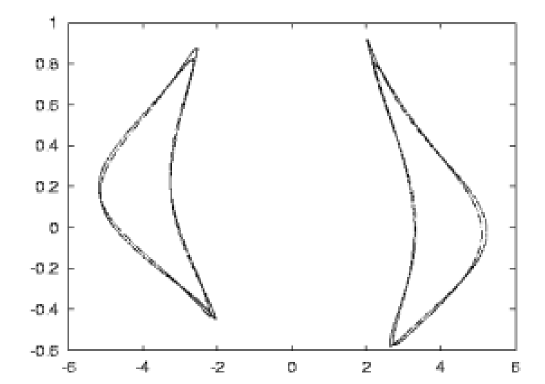
Figure 11: Example 3. Top: The neighborhood of the islands of the Poincaré section; Bottom: Its stochastic zones indicating the absence of integrability.