Derivative moments in turbulent shear flows
Abstract
We propose a generalized perspective on the behavior of high-order
derivative moments in turbulent shear flows by taking account of
the roles of small-scale intermittency and mean shear, in addition
to the Reynolds number. Two asymptotic regimes are discussed with
respect to shear effects. By these means, some existing
disagreements on the Reynolds number dependence of derivative
moments can be explained. That odd-order moments of transverse
velocity derivatives tend not vanish as expected from elementary
scaling considerations does not necessarily imply that small-scale
anisotropy persists at all Reynolds numbers.
PACS: 47.27.Ak, 47.27.Jv ,47.27.Nz
I Introduction
The postulate of local isotropy [1] implies an invariance with respect to spatial rotations of the statistical properties of small scales of turbulence. Even though the large scales are anisotropic in all practical flows, it is thought that the small scales at high Reynolds numbers are shielded from anisotropy because of their separation by a wide range of intermediate scales. At any finite Reynolds number, some residual effects of small-scale anisotropy may linger, but all proper measures of anisotropy are expected to decrease rapidly with Reynolds number. An understanding of the rate at which small scales tend towards isotropy is a basic building block in turbulence theory.
A particularly appealing manner of generating large-scale anisotropy is by a homogeneous shear characterized by a constant shear rate , where is the mean velocity in the streamwise direction , and is the direction of the shear. During the last few years, nearly homogeneous shear flows, both experimental [2, 3, 4] and numerical, [5, 6, 7] have examined the rate at which local isotropy is recovered with respect to the Taylor microscale Reynolds number, . The notation is standard: , is the velocity fluctuation in the longitudinal direction , , , is the kinematic viscosity and denotes a suitably defined average. The discussion has often been focused on the behavior of normalized odd moments of transverse velocity derivatives defined as
| (1) |
where is a positive integer. The velocity derivatives are small-scale quantities, and symmetry considerations of local isotropy demand that the odd moments of transverse velocity derivatives be zero. In practice, they should decrease with relatively rapidly. Though the postulate of local isotropy does not by itself stipulate this rate, simple estimates can be made by retaining the spirit of local isotropy and making further assumptions. Let us assume that the non-dimensional moments depend on some power of the shear, which is the ultimate source of anisotropy in homogeneous shear flows, and non-dimensionalize the shear dependence by a time scale formed by the energy dissipation rate and fluid viscosity ; this non-dimensionalization accords with Kolmogorov’s first hypothesis that small-scale properties depend solely on and . We may then write
| (2) |
where it is further assumed that and is the large scale of turbulence. Lumley [8] considered a linear dependence on the shear (i.e., ). This yields an inverse power of for the decay of all odd moments. The choice accounts for the dependence of the sign of the odd moments on the sign of in a simple manner.
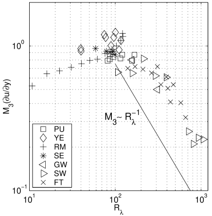
The existing experimental and numerical data on the skewness of the transverse velocity derivative are collected in Fig. 1. Data from any given source seem to fit a power-law of the form
| (3) |
with differing from one set of data to another. Though the power-law is not a particularly good fit for the totality of the data, the average roll-off seems to be less steep than the inverse power discussed above. Atmospheric data at much higher Reynolds numbers [9, 10] are consistent with this slower rate of decay.
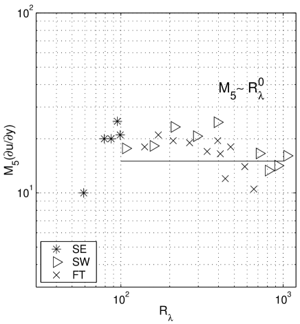
The situation with respect to the hyperksewness, , is as follows. Two independent laboratory experiments in nearly homogeneous shear flows [3, 4] draw different conclusions on the behavior of . On the one hand, Shen and Warhaft [4] find no dependence on in the range between and . On the other hand, Ferchichi and Tavoularis [3] regard their data to be essentially consistent with expectations of local isotropy. (For one perspective on this difference, see Warhaft and Shen [11]). A collection of all known data is given in Fig. 2. The overall impression from the figure is that, while there is probably a weak decreasing trend for , the hyperskewness does not diminish perceptibly even when is as high as 1000. Shen and Warhaft [4] measured the seventh normalized moment of the velocity derivative and found that it increased with instead of decreasing.
Such findings have been interpreted (e.g., Refs. 4 and 5) to mean that, in the presence of large-scale shear, small-scale anisotropy persists to very high Reynolds numbers. The intent of this paper is to clarify, at least partially, the simultaneous role played by shear, intermittency and the Reynolds number—all of which have an impact on trends displayed by odd derivative moments.
We now consider in Sec. II the issue of intermittency versus anisotropy. In Sec. III, we highlight the effects of shear by discussing the limiting cases of large shear and local isotropy, and argue that determines the state of the flow only partially. In Sec. IV the derivative skewness data are plotted in the plane spanned by the non-dimensional shear parameter and , where we use the definition
| (4) |
This broader perspective may help resolve some seemingly contradictory claims on the recovery of isotropy of small scales.
II Intermittency versus anisotropy
A large number of measurements have shown convincingly that high-order moments of small-scale features of turbulence increase with . Consider the longitudinal velocity derivative . The product of its second moment and fluid viscosity is essentially the energy dissipation, which is known to remain independent of when exceeds some moderately high value (see Refs. 14,15). On the other hand, all high-order moments of longitudinal velocity gradients grow with (see, for example, the compilation in Ref. 16 of the data on the flatness factor of ). Sixth and higher order moments increase at increasingly faster rates with . These growths are attributed to the intermittency of small-scale turbulence. At the present level of our understanding, intermittency is independent of anisotropy effects. Therefore, just as the growth of high-order even moments with increasing is unrelated to anisotropy, it is legitimate to ask if, at least in part, the slower-than-expected decay—or even modest growth—of odd moments, may be related to intermittency.
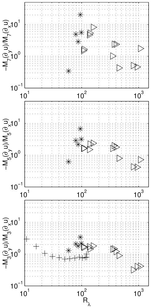
To separate intermittency effects from those of anisotropy, at least in some approximate way, it is useful to plot the ratio . It is plausible to assume that the -growth due to intermittency effects is the same for the moments of and for the moments of , the intermittency effects of odd moments of are cancelled in these ratios by those of . Though this not a rigorous statement, it is useful to see the outcome. Figure 3 shows the results. It is clear, despite large scatter, that all the moments show a tendency to diminish with Reynolds number. The odd-moments in Fig. 3 are normalized by powers of their respective variances. It would have been desirable to plot ratios of unnormalized, or “bare”, moments of the two derivatives, but Ref. 4 does not include those data. In any case, this should not make much difference because is essentially a constant at high Reynolds numbers.
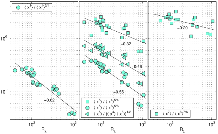
This same issue can be rephrased and reexamined in a somewhat different light. When we consider the moments such as skewness and hyperskewness, we usually normalize them by the appropriate power of the variance of the variable. This is perfectly reasonable for Gaussian or near-Gaussian variables, but not so for intermittent quantities with highly stretched tails. Perhaps a more reasonable alternative is to consider how an odd moment of a certain order varies with respect to the even moment just below or just above, or the geometric mean of those just below and just above. We illustrate the results of this consideration for the third, fifth and seventh order moments of in Fig. 4. The lack of data on the eight moment of makes the analysis of the seventh moment incomplete. Nevertheless, it is clear that all these alternative ways of normalization show substantial decay. It is hard to be precise about the rates of decay, partly because of the large scatter and partly because the incomplete manner in which the seventh moments have been analyzed, but it is conceivable that increasingly high-order moments, within a given normalizing scheme, decay more slowly. At the least, a careful discussion of the restoration of anisotropy requires the proper inclusion of intermittency effects. This is our first point.
III Shear effects in two limiting cases
It is reasonable to suppose that, to a first approximation, the mean shear and the viscosity determine the gross state of the flow. Expressing time units in terms of , length units in terms of the integral length scale , and the mean profile as , we get
| (5) | |||||
| (6) |
where and is unit vector in the streamwise direction . The volume forcing is denoted by . The two parameters may be expected to set the steady state fluctuation level and energy dissipation rate. It also follows that the derived parameters and adjust themselves dynamically, in ways that are understood only partially, to the imposed values of and . We then expect
| (7) | |||||
| (8) |
where and are unknown functions of their arguments.
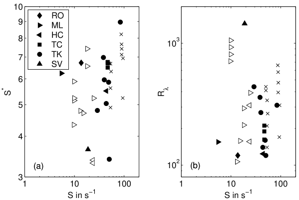
All the homogeneous shear experiments to be discussed below have been done in air. This fixes the viscosity to be approximately constant, so we can test the dependence of and on the shear rate . The relevant plots (Figs. 5 (a) and (b)) show no obvious trend but only large scatter. This scatter may be related in part to the fact that in some of the experiments, leading to nonstationarity. Here is the production of turbulent kinetic energy, defined as for homogeneous shear. In part, it demonstrates that the flow might depend additionally on initial conditions, , or the type of driving of small-scale fluctuations characterized globally by an input energy. From Eq. (5), the latter is given by
| (9) |
We then get more complex relations such as
| (10) | |||||
| (11) |
If we add to Figs. 5 the atmospheric data from Refs. 9 and 10, the situation becomes even more complex. However, it is likely that, in such inhomogeneous flows, one has to take into account secondary factors such as convective effects (though conditions in which they are modest can always be chosen carefully). In laboratory experiments, secondary effects might arise from the use of specific passive or active grids for the generation of turbulence. Further differences can arise when measuring at a fixed point instead of following the downstream evolution. This discussion merely underlines the inadequacy of as the sole indicator of the state of the flow. At the least, we have to possess some knowledge of the other parameters influencing the state of the flow before drawing firm conclusions on the recovery of isotropy.
To keep matters simple, we will focus below on homogeneously sheared flows. Because the initial conditions are not known in all quantifiable details, we shall tentatively stipulate a simple generalization of Eq. (1) in the form
| (12) |
and regard other effects as superimposed “noise” [25]. If so, we should investigate the behavior of the derivative moments by keeping one of the two parameters fixed while varying the other, for example by fixing and varying . This is the topic of the next section. However, it is useful to preface this consideration by examining two limiting behaviors in which some inequalities between and can be established.
A Large shear case
Consider the case of large shear rate for which the coupling of the mean shear to the small-scale flow dominates. In the rapid distortion limit, namely , Eq. (5) becomes linear because the viscous term as well as the term can be dropped, so that any shear rate dependence can be eliminated by the rescaling of the variables, e.g. .
Our dimensional estimates are related to large but finite shear rates. For this case, the term representing the coupling of the turbulent velocity component to the mean shear is important and large in comparison to the nonlinear advective transport. Our situation corresponds to the case in which
| (13) |
For the homogeneous shear flow, we get for the left-hand-side of this equation
| (14) |
In the last step above, we have used the fact that the root-mean-square velocity in the streamwise direction is larger than that in the shear direction, as has been found in all numerical and physical experiments. The term on the right hand side can be estimated roughly as where the scale is characteristic of turbulent velocity gradients, and can therefore be assumed to be of the order of the Taylor microscale, . We then require
| (15) |
With and , and the constant for sufficiently large , we get
| (16) |
In reality, depends weakly on . For example, Sreenivasan [23] has examined the data and concluded that , where , is a good empirical fit. Since this dependence is quite weak, we have taken to be a constant for simplicity. Presumably, if Eq. (14) holds, the effects of shear will always be felt no matter how high the Reynolds number.
B Local isotropy limit
At the other extreme is the case in which local isotropy can be expected, a priori, to prevail. A suitable criterion (see Corrsin [24]) is that a sufficiently large separation should exist between the shear time scale, , and the Kolmogorov time scale, . This can be written as
| (17) |
or as
| (18) |
With and we obtain
| (19) |
The implication is that local isotropy prevails for all substantially smaller than 0.35. For all other conditions, one should expect that the magnitude of will play some role in determining how high an is required for local isotropy to prevail. This explicit dependence on shear has been noted for passive scalars by Sreenivasan and Tavoularis;[26] see their figures 2 and 3.
IV The - phase diagram
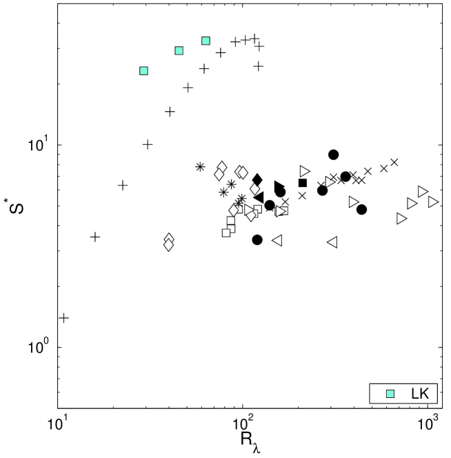
We now plot in Fig. 6 all available data on the skewness of the transverse derivative, , on a phase plane consisting of and . The conventional normalization factors in the definition of are the total turbulent energy and its dissipation rate. This can be done quite readily for the numerical data, but experiments usually provide information only on the streamwise component of the turbulent energy and on the energy dissipation estimate from the local isotropy formula, . The error made in this estimate for the energy dissipation depends[23] on the magnitudes of shear and , but it appears to be a reasonable approximation for the present conditions. We have recalculated for all numerical data the energy dissipation rate as in experiments. It is clear from the figure that there is no simple correlation between the two parameters and .
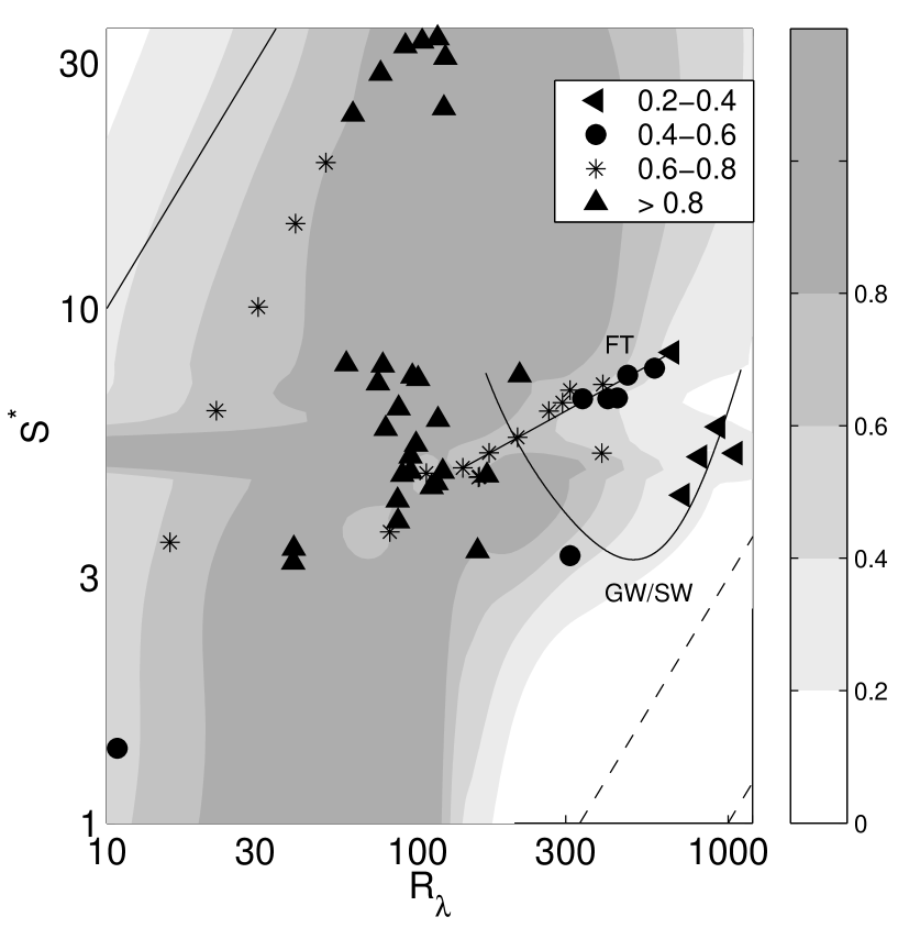
We have replotted the same data in Fig. 7. Different symbols correspond now to different magnitudes of the skewness, as indicated in the legend, and not to different experiments. Superimposed are islands in shades of grey to obtain a rough idea of the surface plot of . We used an interpolation routine with local thin plate splines that can reconstruct a surface from scattered data.[28] The data are sparse in most of the regions of the plane so any surface-fitting routine will introduce some peculiarities. For reasons explained above, we can expect that the derivative skewness will become small in the local isotropy limit (lower right corner) and that the values will grow above 0.8 in the large shear case (upper left corner). Although the latter fact is not reflected by the surface fit because the data points are absent there and almost all data points are in the intermediate region, we think that the surface plot is not unreasonable.
This plot offers additional perspectives. For instance, Fig. 1 is just a projection of the data on to the axis and masks the fundamental effect of the applied shear (among other effects). We have marked in this figure the trends of the data sets of Warhaft and co-workers (parabolic solid line labelled by GW/SW) and of Ferchichi and Tavoularis (straight line labelled by FT), respectively. They show that the two experiments follow different paths: while the Ferchichi-Tavoularis data run directly down the ‘mountain range’, the Shen-Warhaft data seem to run in a kind of spiral around the ‘mountain’, presumably resulting in a slower decay of the skewness when projected on to the axis. Finally, the two limiting regimes of Sec. III are also plotted. The local isotropy limit is not reached for any of the data. The large shear case is reached for very large . A threshold grows when increases; alternatively, local isotropy requires larger if the shear parameter is larger.
V Concluding remarks
Considerable attention has been paid recently to the fact that in shear flows the moments of transverse velocity derivatives do not vanish with Reynolds number as fast as was expected. We have introduced two considerations for interpreting these observations, invoking small-scale intermittency and the magnitude of the shear parameter. These two effects work in combination with the Reynolds numbers in determining the magnitudes of odd moments of velocity derivatives. The fact that the odd moments, when normalized by an appropriate power of the variance (a procedure steeped in studies of Gaussian processes), decay more slowly than expected should not be considered a priori as incontrovertible evidence against local isotropy. We believe that the broader perspective of this paper may explain some seeming contradictions that exist in the literature.
The conclusions we draw in this paper would be more definitive if the data spanned much higher Reynolds number range. This can be done with adequate resolution only in atmospheric flows at present. The existing measurements are in conformity with the discussion here, but it is difficult to be definitive because of the usual problems that often exist in atmospheric measurements. On the other hand, it seems quite feasible in numerical simulations to fix the Reynolds number and vary the shear parameter, even though the Reynolds number range may be limited. Such a study will tell us more about the restoration (or otherwise) of small-scale isotropy.
In the recent past, various efforts have been made to understand the effects of anisotropy through an SO(3) decomposition of structure functions and other tensorial objects (see Ref. 29 for the basic theoretical idea and Refs. 30-32 for implementations of the idea and further references). The method offers a transparent way of determining the degree of anisotropy in turbulent statistics. The relation between that effort and the present global picture needs to be explored.
ACKNOWLEDGMENTS
We thank A. Pumir and Z. Warhaft for providing raw numbers for some of their published figures, and acknowledge fruitful discussions with A. Bershadskii, S. Chen, J. Davoudi, B. Eckhardt, R.J. Hill, S. Kurien, S.B. Pope, I. Procaccia (especially) and Z. Warhaft. J.S. was supported by the Feodor-Lynen Fellowship Program of the Alexander-von-Humboldt Foundation and Yale University. The work was supported by the NSF grant DMR-95-29609. Numerical calculations were done on a Cray T90 at the John von Neumann-Institut für Computing and on the IBM Blue Horizon at the San Diego Supercomputer Center. We are grateful to both institutions for support.
REFERENCES
- [1] A. N. Kolmogorov, “The local structure of turbulence in incompressible viscous fluid for very large Reynolds numbers,” Dokl. Akad. Nauk SSSR 30, 301 (1941).
- [2] S. Garg and Z. Warhaft, “On small scale statistics in a simple shear flow,” Phys. Fluids 10, 662 (1998).
- [3] M. Ferchichi and S. Tavoularis, “Reynolds number effects on the fine structure of uniformly sheared turbulence,” Phys. Fluids 12, 2942 (2000).
- [4] X. Shen and Z. Warhaft, “The anisotropy of the small scale structure in high Reynolds number () turbulent shear flow,” Phys. Fluids 12, 2976 (2000).
- [5] A. Pumir, “Turbulence in homogeneous shear flows,” Phys. Fluids 8, 3112 (1996).
- [6] J. Schumacher and B. Eckhardt, “On statistically stationary homogeneous shear turbulence,” Europhys. Lett. 52, 627 (2000).
- [7] J. Schumacher, “Derivative moments in stationary homogeneous shear turbulence,” J. Fluid Mech. 441, 109 (2001).
- [8] J. L. Lumley, “Similarity and the turbulent energy spectrum,” Phys. Fluids 10, 855 (1967).
- [9] B. Dhruva and K. R. Sreenivasan, “Is there scaling in high-Reynolds-number turbulence?,” Prog. Theo. Phys. Supp. 130, 103 (1998).
- [10] S. Kurien and K. R. Sreenivasan, “Anisotropic scaling contributions to high-order structure functions in high-Reynolds-number turbulence,” Phys. Rev. E 62, 2206 (2000).
- [11] Z. Warhaft and X. Shen, “Some comments on the small scale structure of turbulence at high Reynolds number,” Phys. Fluids 13, 1532 (2001).
- [12] B. L. Sawford and P. K. Yeung, “Eulerian acceleration statistics as a discriminator between Lagrangian stochastic models in uniform shear flow,” Phys. Fluids 12, 2033 (2000).
- [13] M. M. Rogers, P. Moin, and W. C. Reynolds, “The structure and modeling of the hydrodynamic and passive scalar fields in homogeneous turbulent shear flow,” Report No. TF-25, Department of Mechanical Engineering, Stanford University (1986).
- [14] K. R. Sreenivasan, “On the scaling of the turbulence energy dissipation rate,” Phys. Fluids 27, 1048 (1984).
- [15] K. R. Sreenivasan, “An update on the dissipation rate in homogeneous turbulence,” Phys. Fluids 10, 528 (1998).
- [16] K. R. Sreenivasan and R. A. Antonia, “The phenomenology of small-scale turbulence,” Annu. Rev. Fluid Mech. 29, 435 (1997).
- [17] W. G. Rose, “Results of an attempt to generate a homogeneous turbulent shear flow,” J. Fluid Mech. 25, 97 (1966).
- [18] P. J. Mulhearn and R .E. Luxton, “The development of turbulence structure in a uniform shear flow,” J. Fluid Mech. 68, 577 (1975).
- [19] V. G. Harris, J. A. H. Graham, and S. Corrsin, “Further experiments in nearly homogeneous turbulent shear flow,” J. Fluid Mech. 81, 657 (1977).
- [20] S. Tavoularis and S. Corrsin, “Experiments in nearly homogeneous turbulent shear flow with a uniform mean temperature gradient. Part 1,” J. Fluid Mech. 104, 311 (1981).
- [21] S. Tavoularis and U. Karnik, “Further experiments on the evolution of turbulent stresses and scales in uniformly sheared turbulence,” J. Fluid Mech. 204, 457 (1989).
- [22] S. G. Saddoughi and S. V. Veeravalli, “Local isotropy in turbulent boundary layers at high Reynolds number,” J. Fluid Mech. 268, 333 (1994).
- [23] K. R. Sreenivasan, “The energy dissipation rate in turbulent shear flows,” in Developments in Fluid Mechanics and Aerospace Sciences, edited by S.M. Deshpande, A. Prabhu, K.R. Sreenivasan & P.R. Viswanath, Interline Publishers, pp. 159–190, 1995.
- [24] S. Corrsin, “Local isotropy in turbulent shear flow,” N.A.C.A. Res. Memo. RM 58B11 (1958).
- [25] In the context of Kolmogorov’s refined similarity hypotheses, a similar suggestion was made by P. Gualtieri, C. M. Casciola, R. Benzi, G. Amati and R. Piva, “Scaling laws and intermittency in homogeneous shear flow,” Phys. Fluids 14, 583 (2002). These authors considered the parameter plane set up by two length scales, both of which contained the shear length . Thus, they were not separating shear effects from other effects.
- [26] K. R. Sreenivasan and S. Tavoularis, “On the skewness of the temperature derivative in turbulent flows,” J. Fluid Mech. 101, 783 (1981).
- [27] M. J. Lee, J. Kim, and P. Moin, “Structure of turbulence at high shear rate,” J. Fluid Mech. 216, 561 (1990).
- [28] R. Franke, “Smooth interpolation of scattered data by local thin plate splines,” Comput. Math. Appl. 8, 273 (1982).
- [29] I. Arad, V. S. L’vov, and I. Procaccia, “Correlation functions in isotropic and anisotropic turbulence: The role of the symmetry group,” Phys. Rev. E 59, 6753 (1999).
- [30] I. Arad, B. Dhruva, S. Kurien, V.S. L’vov, I. Procaccia and K.R. Sreenivasan, “Extraction of anisotropic contributions in turbulent flows,” Phys. Rev. Lett. 81, 5330 (1998).
- [31] I. Arad, L. Biferale, I. Mazzitelli and I. Procaccia, “Disentangling scaling properties in anisotropic and inhomogeneous turbulence,” Phys. Rev. Lett. 82, 5040 (1999).
- [32] S. Kurien and K.R. Sreenivasan, ”Measures of anisotropy and the universal properties of turbulence”, in Les Houches Summer School Proceedings 2000, Springer-EDP Publishers, pp. 53-111, 2001.