Stages of Energy Transfer in the FPU Model

Joseph A. Biello, Peter R. Kramer, and Yuri V. Lvov

Department of Mathematical Sciences

Rensselaer Polytechnic Institute

301 Amos Eaton Hall

110 8th Street

Troy, NY 12180, USA

Abstract. The (alpha) version of the Fermi-Pasta-Ulam is revisited through direct numerical simulations and an application of weak turbulence theory. The energy spectrum, initialized with a large scale excitation, is traced through a series of distinct qualitative phases en route to eventual equipartition. Weak turbulence theory is applied in an attempt to provide an effective quantitative description of the evolution of the energy spectrum. Some scaling predictions are well-confirmed by the numerical simulations.

1. Introduction

One of the very first uses of electronic computing machines was Fermi, Pasta, and Ulam’s simulation of wave propagation in a weakly nonlinear lattice model [16]. They were expecting to observe that the weak coupling of the normal modes of the system would induce a redistribution of energy from an initial large-scale excitation to an equal sharing (equipartition) of energy among all normal modes after some time. As is well known, they were instead surprised to see the system display regular behavior characteristic of integrable systems, with the initial state recurring on a rather short time scale. This discovery shifted attention to its explanation and ramifications [19, 32] for several decades. In the last two decades, however, the Fermi-Pasta-Ulam (FPU) model has once again been utilized as a test model for numerically illustrating and exploring standard concepts in statistical mechanics [10]. The peculiar near-integrable behavior observed by Fermi, Pasta, and Ulam is characteristic of their model only for systems which are sufficiently small in size and energy. There exist well-defined regimes for which the FPU model is weakly nonlinear but stochastic [11, 24, 35], and it is in these regimes that one can hope to connect the outcome of direct numerical simulations with statistical mechanical concepts [10], such as relaxation to equipartition [10, 15, 31, 36], entropy production [10, 14, 15, 23, 31, 36], chaos as manifested by positive Lyapunov exponents [2, 10, 13, 35, 37], universal behavior of statistical functions [14, 15, 23, 36, 37] and virial relations [3, 4]. The reason for using the FPU model for this purpose is that it is one of the simplest and most natural one-dimensional nonlinear models for statistical mechanics which can be conceived. An interesting alternative of comparable simplicity which has been the subject of recent research is the truncated Burgers model [1, 28, 30].

Our intent is to use the FPU model to scrutinize a “weak turbulence” (WT) theory, a nonequilibrium statistical mechanical theory which attempts to describe the dynamical energy transfer among normal modes in a weakly nonlinear, dispersive, extended system [5, 6, 18, 20, 33, 34, 40]. The theory has been developed over the last four decades to describe the energy transfer in wave dynamics primarily in fluids and plasmas [33, 34, 40], among other novel applications such as semiconductors [25, 26, 27].

These systems are generally too complex for effective comparison of the weak turbulence theory with direct numerical simulations. Only in recent years has a simple one-dimensional model with features representative of such fluid systems been explored by Cai, Majda, McLaughlin, and Tabak [7, 8, 29] to examine the assumptions underlying WT theory. We propose to apply the FPU model for a similar purpose, though the issues on which we focus are distinct. The implications of our studies for the framework of WT theory will be taken up in other works [21].

Here we will present the content of our findings as they inform the relaxation process in the FPU model in the stochastic but weakly nonlinear regime. We will restrict attention to the $\alpha$ version of FPU model, which has purely quadratic nonlinearity in the equations of motion (Section 2). The $\beta$ version (with cubic nonlinearity) seems to be the subject of more work [3, 15, 22, 31, 35, 36], but the $\alpha$ version has attributes which make it more suitable for a first test case for WT theory. Most of the previous statistical mechanical work concerning the FPU models of which we are aware focuses primarily on computing particular statistical measures of the process, such as the time until equipartition is reached [15, 36], the Lyapunov exponents characterizing the degree of chaos [10, 13, 35, 37], or more exotic quantities characterizing the geometry of the trajectories [2, 11]. Another recent line of research has been tracing the path of energy transfer starting from a small set of excited modes [12, 38, 39]. Because the WT theory has the potential to describe the process of energy transfer in the system from beginning to end, we have instead sought to characterize the entire evolution of the energy spectrum from large-scale excitation to eventual equipartition. We will consider the energy transfer in spectral terms, in contrast to the physical space viewpoint developed for the $\beta$-FPU model by Lichtenberg and coworkers [31].

The energy spectrum in the $\alpha$-FPU model approaches equilibrium through a series of qualitatively distinct phases which we illustrate in Section 3. At the initial time, the energy is concentrated in a small set of low-wavenumber modes. This energy then proceeds to higher wavenumbers first through a standard superharmonic cascade, and then shifts to a nonlocal transfer of energy from low wavenumbers to a band of intermediate wavenumber modes. The energy in this intermediate wavenumber band then rolls back through an inverse cascade to lower wavenumbers again. This process then creates approximate equipartition only over a set of modes extending up to a cutoff wavenumber, beyond which the energy content falls off exponentially rapidly [9, 17]. We refer to the location of the transition between the flat and rapidly decaying parts of the energy spectrum as the “knee.”

After presenting this pictorial “life history” of a large-scale excitation in the $\alpha$-FPU system, we present in Section 4 some specific quantitative predictions of WT theory and compare them with the numerical results. At the coarsest level, WT theory suggests the presence of two nonlinear time scales. Over the first nonlinear time scale, energy is exchanged through triads of modes which remain resonant over this time scale. A consideration of the resonances in the dispersion relation indicates that only modes of sufficiently small wavenumber can participate in nearly resonant triads [37]. This in turn suggests that this triad interaction phase should correspond to the formation of the partial equipartition up to the knee. The subsequent relaxation of the energy spectrum to global equipartition requires the slower energy exchange among resonant quartets of normal modes, which are much more abundant. Our present focus is on the triad interaction phase.

An adaptation of the WT theory allows predictions of both the order of magnitude of the time scale and the location of the knee which agree excellently with direct numerical simulation.

2. Fermi-Pasta-Ulam Model

The Fermi-Pasta-Ulam (FPU) model is a model for a one-dimensional collection of particles with massless, weakly anharmonic (nonlinear) springs connecting them to each other. Letting $\{q_{j}\}_{j=1}^{N}$ and $\{p_{j}\}_{j=1}^{N}$ denote the position and momentum coordinates of an $N$-particle chain, we can define the FPU model Hamiltonian:

$$H=\sum\limits_{j=1}^{N}\left(\frac{p_{j}^{2}}{2m}+\kappa\frac{(q_{j}-q_{j+1})^{2}}{2}+\alpha\frac{(q_{j}-q_{j+1})^{3}}{3}+\beta\frac{(q_{j}-q_{j+1})^{4}}{4}\right)$$ (1)

Here we assumed periodic boundary conditions $p_{N+1}=p_{1}$ and $q_{N+1}=q_{1}$. Equivalently, the beads are connected in a circular arrangement. The parameter $m$ denotes the particle mass, while $\kappa$, $\alpha$, and $\beta$ are coefficients involving the spring properties.

The equations of motion are the standard Hamilton’s equations:

$$\dot{q}_{j}=\frac{\partial{{H}}}{\partial p_{j}},\ \ \dot{p}_{j}=-\frac{\partial{{H}}}{\partial q_{j}}$$ (2)

We will here focus on the $\alpha$-FPU model for which $\alpha\neq 0$ and the quartic term is absent ($\beta=0$). We nondimensionalize the system with respect to the spring constant $\kappa$, the mass $m$, and the energy density $H/N$. Retaining the original symbols for the nondimensionalized variables $p_{j}$ and $q_{j}$, we obtain the nondimensionalized Hamiltonian and equations of motion:

$${\mathcal{H}} = \frac{1}{2}\sum\limits_{j=1}^{N}\left({p_{j}^{2}}+(q_{j}-q_{j+1})^{2}\right)+\frac{\epsilon}{3}\sum\limits_{j=1}^{N}(q_{j}-q_{j+1})^{3}$$ (3)

$$\dot{q}_{j} = p_{j}$$

$$\dot{p}_{j} = \left(q_{j-1}-2q_{j}+q_{j+1}\right)\left(1+\epsilon(q_{j-1}-q_{j+1})\right)$$

Our choice of nondimensionalization implies that

$${\mathcal{H}}=N$$ (4)

for all times. The fundamental nondimensional parameter measuring the strength of the nonlinearity is

$$\epsilon\equiv\alpha\sqrt{\frac{H}{N}}.$$

In order to study the transfer of energy among different scales, we represent the system in terms of Fourier modes:

$$\left(\begin{array}[]{c}q_{l}\\ p_{l}\end{array}\right)=\frac{1}{N}\sum\limits_{k=-\frac{N}{2}+1}^{N/2}\left(\begin{array}[]{c}Q_{k}\\ P_{k}\end{array}\right)\exp{\left(\frac{-2\pi ikl}{N}\right)}$$ (9)

$$\left(\begin{array}[]{c}Q_{k}\\ P_{k}\end{array}\right)=\sum\limits_{l=1}^{N}\left(\begin{array}[]{c}q_{l}\\ p_{l}\end{array}\right)\exp{\left(\frac{2\pi ikl}{N}\right)}$$ (14)

The Hamiltonian in the new variables reads

$${\mathcal{H}} = \frac{1}{2N}\sum\limits_{k=-\frac{N}{2}+1}^{\frac{N}{2}}\left[|P_{k}|^{2}+\omega_{k}^{2}|Q_{k}|^{2}\right]$$

$$\qquad+\frac{\epsilon}{3N^{2}}\sum\limits_{k_{1},k_{2},k_{3}=-\frac{N}{2}+1}^{\frac{N}{2}}V_{k_{1},k_{2},k_{3}}Q_{k_{1}}Q_{k_{2}}Q_{k_{3}}\delta_{k_{1}+k_{2}+k_{3},0},$$

where the dispersion relation is given by

$$\omega_{k}=2\left|\sin{\left(\frac{\pi k}{N}\right)}\right|,$$ (16)

the nonlinear coupling coefficients are

$$V_{k_{1},k_{2},k_{3}}=-i\,\mathrm{sgn}\,(k_{1}k_{2}k_{3})\omega_{k_{1}}\omega_{k_{2}}\omega_{k_{3}},\ \ \ k_{1}+k_{2}+k_{3}=0,$$ (17)

and

$$\delta_{i,j}\equiv\begin{cases}1&\mbox{if }i=j\mod N,\\ 0&\mbox{else.}\end{cases}$$

is a periodized version of the Kronecker delta function.

To quantify the amplitude of activity of the FPU chain at different scales, we define the harmonic energy contribution of each Fourier mode:

$$E_{h,k}(t)\equiv\frac{1}{2N}\left[|P_{k}|^{2}+\omega_{k}^{2}|Q_{k}|^{2}\right].$$

Energy equipartition implies $E_{h,k}$ is independent of $k$ (and $t$). The total harmonic contribution to the energy is

$$E_{h}(t)\equiv\sum_{k=-N/2+1}^{N/2}E_{h,k}(t).$$

3. Numerical Simulation of Relaxation from Initial Large-Scale Excitation

The equations of motion in (3) were integrated using a fourth order Runge-Kutta time stepping routine. Since the equations are local in physical space, all calculations were performed there. FFTs were employed only for data analysis. All simulations conserved energy to within $10^{-3}$ after the full length of the simulation whereas total momentum and particle position were conserved to machine accuracy. With a specified number of excited initial modes, the amplitude and phase of the Fourier coefficients are each chosen from a uniform distribution so that, on average, each mode would be initialized with the same energy. The initial data is then normalized according to Eq. (4). The results of all experiments are averaged over 10–20 independent realizations of the initial data; these relatively small ensembles proved sufficient to elucidate the results.

Figure 1 shows a sequence of ensemble averaged spectra for a lattice of length $N=512$ and nonlinearity strength $\epsilon=0.03$ at times $t=0$, $50$, $100$, $200$, $400$, $1000$, $2500$, $5000$, $10^{4}$, displaced for ease of viewing. The evolution proceeds from a set of $50$ initially excited modes to a superharmonic cascade to all wave numbers with exponentially decreasing energy by $t=50$. By $t=100$ the initial band has transferred much of its energy to intermediate wavenumbers, forming a slight hump. Thereafter, this hump of energy rolls back via an inverse cascade to low wavenumbers. At $t=10^{4}$, the energy spectrum exhibits a plateau at low wavenumbers and an exponential falloff at higher wavenumbers. This last spectrum is the motivation for the term “knee”, below which the waves are in equipartition and above which they are not substantially excited [9, 17]. After $t=10^{4}$ the spectrum evolves over much longer time scales, eventually arriving at equipartition throughout.

Figure 2 shows a similar experiment with a larger ensemble (20 realizations), $N=512$ and $\epsilon=0.05$. The initial excitation band is very much smaller, including only 20 waves. Again spectra are displaced and in this example are shown at $t=0,10^{3},2\times 10^{3},4\times 10^{3},8\times 10^{3},2\times 10^{4},5\times 10^{4},10^{5}$. Energy is driven first to an intermediate range of wavenumbers which saturate. Subsequently, an inverse cascade of energy extends the band of equilibration backward to lower wavenumbers until $t\sim 8\times 10^{3}$, at which point only the lowest wavenumber has yet to reach equipartition. At $t=5\times 10^{4}$ the spectrum is quasi-stationary, equipartition being achieved among all wavenumbers less than $k_{\mathrm{knee}}$. The energy in larger wavenumbers decreases rapidly. At $t=10^{5}$ the highest modes begin to acquire energy. Eventually the whole spectrum will arrive at equipartition; this process is outside of the scope of the current work.

4. Scaling Predictions

A renormalized WT theory derived in [21] predicts that significant three wave interaction should occur in a band

$$|k|\leq k_{\mathrm{knee}}\sim N\sqrt{\epsilon}$$ (18)

on a time scale

$$T_{3}\sim\epsilon^{-3/2}.$$ (19)

This theory only applies when the lattice size is large enough ($N\gg\epsilon^{-1/2}$) and the number of initially excited modes is an order unity fraction of the knee width $k_{\mathrm{knee}}$, so that the renormalized energy spectrum remains self-consistently of order unity during this phase of evolution.

A useful statistical measure for our purposes is the spectral entropy, defined as

$$S(t)=-\sum_{k}\frac{E_{h,k}(t)}{E_{h}(t)}\log\left(\frac{E_{h,k}(t)}{E_{h}(t)}\right).$$

This provides a measure of the effective number of excited normal modes at any given time, $n_{\mathrm{eff}}(t)\equiv e^{S(t)}$ [10, 14, 24, 31, 36]. Figure 3 shows rescaled plots of this spectral entropy as a function of time. The onset of the quasi-stationary phase, after the end of the three-wave evolution, is clearly evident. The knee width $k_{\mathrm{knee}}\approx 1.5N\sqrt{\epsilon}$ is determined as an average of $n_{\mathrm{eff}}$ over a time window shortly after the entropy ends its rapid rise. This scaling relationship is robust against various choices of initial bandwidth excitations. The time to reach partial equipartition $T_{3}$, however, does depend sensitively on the choice of initial data. As discussed above, the WT theory producing the scaling prediction (19) assumes the initial data is excited over a band of wavenumbers which is an order unity fraction of the knee width. To test the prediction (19), then, we choose the system to have initially $\frac{1}{2}k_{\mathrm{knee}}\approx 0.75N\sqrt{\epsilon}$ excited modes. (The evolution depicted in Figure 1 comes from initial data of this form, whereas the example in Figure 2 was initialized with a considerably smaller band of excited modes). The time scale $T_{3}$ for the system to reach partial equipartition is determined automatically as the first time at which $n_{\mathrm{eff}}(t)$ achieves the value $k_{\mathrm{knee}}=1.5N\sqrt{\epsilon}$.

4.1. Effect of strength of nonlinearity

Ensembles of FPU lattices with lattice length $N=512$ were integrated for values of $\epsilon$ ranging from $10^{-3}$ to $10^{-1}$. Figures 4 and 5 show excellent agreement with the $\epsilon$ scaling dependences (18) and (19) predicted by the renormalized WT theory. The scaling $k_{\mathrm{knee}}\sim\epsilon^{1/2}$ had also been previously observed in [37].

4.2. Effect of lattice size

The renormalized WT theory also predicts that the knee width should scale with lattice size (Eq. (18)) whereas the three wave time scale should not (Eq. (19)). These properties are compatible with a thermodynamic limit. In figure 3 the logarithm of the fraction of modes to the total lattice size is plotted against time for seven ensembles of experiments with increasing lattice size $N=32,64,128,256,1024,2048,4096$, and fixed $\epsilon=0.1$. These experiments were again initialized with half the number of modes of the predicted knee. Three features of this plot stand out most clearly. First, the spectral entropy follows a universal evolution [14, 36] for lattice sizes larger than $N=128$. Secondly, the number of excited modes exponentially increases with time prior to three wave equilibrium. Finally, for $N=32$ (where the initial number of excited modes is approximately $7$) there is no equilibrium, but rather quasi-periodic behavior. In fact, a shadow of this behavior is present for $N=64$ and $128$ also. These are reminiscent of the integrability discovered in Fermi, Pasta and Ulam’s original work [16], and indicate the breakdown of the WT theory scaling predictions for small lattice sizes.

5. Conclusion

We have emphasized some of the long-lived transient features of the evolution of the energy spectrum in the $\alpha$-FPU model. Weak turbulence theory has been successful in predicting scaling exponents concerning the achievement of partial equipartition. In the future, we will endeavor to explain other dynamical aspects, such as the formation of the energy hump at intermediate wavenumbers and subsequent inverse cascade, in similar quantitative terms.

6. Acknowledgements

The authors would like to thank David Cai and Gregor Kovačič for helpful discussions. JAB is supported by an NSF VIGRE postdoctoral research fellowship DMS 9983646, PRK is supported by an NSF grant DMS-A11271, and YVL is partially supported by NSF Career grant DMS 0134955 and ONR YIP grant N000140210528.

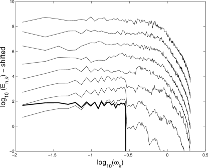
Figure 1. Temporal evolution of spatial FPU energy spectrum versus mode frequency for an ensemble of experiments on a lattice of length $N=512$. Subsequent spectra are shifted upward for ease of viewing. Times are, initial (thick line), $t=50,100,200,400,1000,2500,5000,10^{4}$. Intermediate times show an inverse cascade whereas late times clearly show a knee, above which energy decays rapidly.

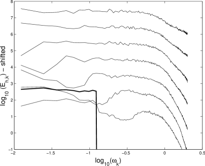
Figure 2. Temporal evolution of spatial FPU energy spectrum with lattice length $N=512$. Subsequent spectra are shifted upward for ease of viewing. Times are, initial (thick line), $t=10^{3},2\times 10^{3},4\times 10^{3},8\times 10^{3},2\times 10^{4},5\times 10^{4},10^{5}$ A narrower initial spectrum yields a more pronounced inverse cascade at intermediate times. At late times high wavenumbers begin to acquire more energy.

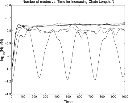
Figure 3. $\log_{10}(n_{\mathrm{eff}}(t)/N)$ versus time for lattice lengths $N=32,64,128,256,1024,2048,4096$, $\epsilon=0.1$. The simulations with large lattice length lie along one another in confirmation of the universal scaling predictions (18) and (19). Lattices with $N\leq 128$ show some mild quasi-periodicity whereas the simulation $N=32$ clearly shows the quasi-periodic behavior of the original FPU simulations [16].

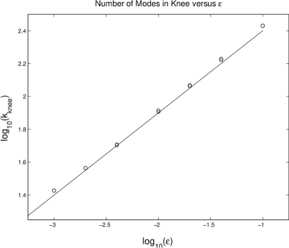
Figure 4. Knee width, $\log_{10}(k_{\mathrm{knee}})$ versus $\log_{10}(\epsilon)$ for $N=512$ and initial data chosen at half the predicted knee width. The line represents the scaling law $k_{\mathrm{knee}}=1.5\epsilon^{1/2}N$.

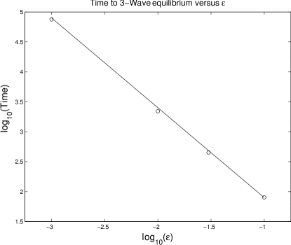
Figure 5. Time to three-wave equilibrium, $\log_{10}(T_{3})$ versus $\log_{10}(\epsilon)$ for $N=512$ and initial data chosen at half the predicted knee width. The line represents the scaling law $T_{3}=2.5\varepsilon^{-3/2}$.

References

- [1] Rafail V. Abramov, Gregor Kovačič, and Andrew J. Majda. Hamiltonian structure and statistically relevant conserved quantities. to appear in Communications on Pure and Applied Mathematics, 2002.
- [2] Carlo Alabiso and Mario Casartelli. Quasi-harmonicity and power spectra in the FPU model. J. Phys. A, 33(5):831–839, 2000.
- [3] Carlo Alabiso and Mario Casartelli. Normal modes on average for purely stochastic systems. J. Phys. A, 34:1223–1230, 2001.
- [4] Carlo Alabiso, Mario Casartelli, and Paolo Marenzoni. Nearly separable behavior of Fermi-Pasta-Ulam chains through the stochasticity threshold. J. Statist. Phys., 79(1/2):451–471, 1995.
- [5] D. J. Benney and P. Saffman. Nonlinear interaction of random waves in a dispersive medium. Proc. Roy. Soc. London, 289(1418):301–320, January 25 1966.
- [6] J. Benney and A. C. Newell. Random wave closure. Stud. in Appl. Math., 48:1, 1969.
- [7] David Cai, Andrew J. Majda, David W. McLaughlin, and Esteban G. Tabak. Spectral bifurcations in dispersive wave turbulence. Proc. Nat. Acad. Sci. USA, 96(25):14216–14221, December 7 1999.
- [8] David Cai, Andrew J. Majda, David W. McLaughlin, and Esteban G. Tabak. Dispersive wave turbulence in one dimension. Phys. D, 152/153:551–572, 2001. Advances in nonlinear mathematics and science.
- [9] A. Carati and L. Galgani. Theory of dynamical systems and the relations between classical and quantum mechanics. Found. Phys., 31(1):69–87, 2001. Invited papers dedicated to Martin C. Gutzwiller, Part II.
- [10] Lapo Casetti, Monica Cerruti-Sola, Marco Pettini, and E. G. D. Cohen. The Fermi-Pasta-Ulam problem revisited: stochasticity thresholds in nonlinear Hamiltonian systems. Phys. Rev. E (3), 55(6, part A):6566–6574, 1997.
- [11] Monica Cerruti-Sola and Marco Pettini. Phase space geometry and stochasticity thresholds in hamiltonian dynamics. Phys. Rev. E, 62(5):6078–6081, November 2000.
- [12] G. Christie and B. I. Henry. Resonance energy transfers in the induction phenomena in quartic Fermi-Pasta-Ulam. Phys. Rev. E, 58(3):3045–3054, September 1998.
- [13] Thierry Dauxois, Stefano Ruffo, and Alesandro Torcini. Modulational estimate for the maximal Lyapunov exponent in Fermi-Pasta-Ulam chains. Phys. Rev. E, 56(6):R6229–R6232, December 1997.
- [14] J. De Luca, A. J. Lichtenberg, and S. Ruffo. Universal evolution to equipartition in oscillator chains. Phys. Rev. E, 54(3):2329–2333, September 1996.
- [15] J. De Luca, A. J. Lichtenberg, and S. Ruffo. Finite times to equipartition in the thermodynamic limit. Phys. Rev. E, 60(4):3781–3786, October 1999.
- [16] E. Fermi, J. Pasta, and S. Ulam. Studies of nonlinear problems. In Alan C. Newell, editor, Proceedings of the Summer Seminar, sponsored by the American Mathematical Society and the Society for Industrial and Applied Mathematics, held at Clarkson College of Technology, Potsdam, N.Y., 1972, pages 143–156. American Mathematical Society, Providence, R.I., 1974. Los Alamos Sci. Lab. Rep. No. LA-1940 (1955).
- [17] Luigi Galgani, Antonio Giorgilli, Andrea Martinoli, and Stefano Vanzini. On the problem of energy equipartition for large systems of the Fermi-Pasta-Ulam type: analytical and numerical estimates. Phys. D, 59(4):334–348, 1992.
- [18] K. Hasselmann. On the non-linear energy transfer in a gravity-wave spectrum. I. General theory. J. Fluid Mech., 12:481–500, 1962.
- [19] Eryk Infeld and George Rowlands. Nonlinear waves, solitons and chaos. Cambridge University Press, Cambridge, second edition, 2000.
- [20] B. B. Kadomtsev. Plasma turbulence. Academic Press, New York, 1965.
- [21] Peter R. Kramer, Joseph A. Biello, and Yuri Lvov. Application of weak turbulence theory to fpu model. submitted to this volume, September 2002.
- [22] Xavier Leoncini and Alberto Verga. Dynamical approach to the microcanonical ensemble. Phys. Rev. E, 64(6):066101, November 7 2001.
- [23] C. Y. Lin, S. N. Cho, C. G. Goedde, and S. Lichter. When is a one-dimensional lattice small? Phys. Rev. Lett., 82(2):259–262, January 11 1999.
- [24] Roberto Livi, Marco Pettini, Stefano Ruffo, Massimo Sparpaglione, and Angelo Vulpiani. Equipartition threshold in nonlinear large Hamiltonian systems: The Fermi-Pasta-Ulam. Phys. Rev. A, 31(2):1039–1045, February 1985.
- [25] Y. V. Lvov, R. Binder, and A. C. Newell. Quantum weak turbulence with applications to semiconductor lasers. Physica D, 121:317–343, 1998.
- [26] Yuri V. Lvov. Finite flux solutions of the quantum Boltzmann equation and semiconductor lasers. Phys. Rev. Lett., 84(9):1894–1897, February 28 2000.
- [27] Yuri V. Lvov and Alan C. Newell. Semiconductor lasers and kolmogorov spectra. Phys. Lett. A, 235:499–503, November 17 1997.
- [28] A. Majda and I. Timofeyev. Statistical mechanics for truncations of the burgers-hopf equation: A model for intrinsic stochastic behavior with scaling. Milan J. Math., 70(1):39–96, 2002.
- [29] A. J. Majda, D. W. McLaughlin, and E. G. Tabak. A one-dimensional model for dispersive wave turbulence. J. Nonlinear Sci., 7(1):9–44, 1997.
- [30] Andrew J. Majda and Ilya Timofeyev. Remarkable statistical behavior for truncated Burgers-Hopf dynamics. Proc. Natl. Acad. Sci. USA, 97(23):12413–12417 (electronic), 2000.
- [31] V. V. Mirnov, A. J. Lichtenberg, and H. Guclu. Chaotic breather formation, coalescence, and evolution to energy equipartition in an oscillatory chain. Physica D, 157:251–282, 2001.
- [32] Alan C. Newell. Solitons in mathematics and physics. Society for Industrial and Applied Mathematics (SIAM), Philadelphia, Pa., 1985.
- [33] Alan C. Newell. Wave turbulence is almost always intermittent at either small or large scales. To appear in Stud. in Appl. Math, 2001.
- [34] Alan C. Newell, Sergey Nazarenko, and Laura Biven. Wave turbulence and intermittency. Phys. D, 152/153:520–550, 2001. Advances in nonlinear mathematics and science.
- [35] P. Poggi and S. Ruffo. Exact solutions in the FPU oscillator chain. Phys. D, 103(1-4):251–272, 1997. Lattice dynamics (Paris, 1995).
- [36] Pietro Poggi, Stefano Ruffo, and Holger Kantz. Shock waves and time scales to reach equipartition in the Fermi-Pasta-Ulam model. Phys. Rev. E (3), 52(1, part A):307–315, 1995.
- [37] D. L. Shepelyanksy. Low-energy chaos in the Fermi-Pasta-Ulam problem. Nonlinearity, 10:1331–1338, 1997.
- [38] K. Yoshimura. Mode instability in one-dimensional anharmonic lattices: Variational equation approach. Phys. Rev. E, 59(3):3641–3654, March 1999.
- [39] K. Yoshimura. Parametric resonance energy exchange and induction phenomenon in a one-dimensional nonlinear oscillator chain. Phys. Rev. E (3), 62(5, part A):6447–6461, 2000.
- [40] V. E. Zakharov, V. S. L’vov, and G. Falkovich. Kolmogorov Spectra of Turbulence, volume 1. Springer-Verlag, Berlin, 1992.