Sand stirred by chaotic advection

Abstract

We study the spatial structure of a granular material, $N$ particles subject to inelastic mutual collisions, when it is stirred by a bidimensional smooth chaotic flow. A simple dynamical model is introduced where four different time scales are explicitly considered: i) the Stokes time, accounting for the inertia of the particles, ii) the mean collision time among the grains, iii) the typical time scale of the flow, and iv) the inverse of the Lyapunov exponent of the chaotic flow, which gives a typical time for the separation of two initially close parcels of fluid. Depending on the relative values of these different times a complex scenario appears for the long-time steady spatial distribution of particles, where clusters of particles may or not appear.

Many different physical processes can be studied in the general framework of transport of finite-size particles by an external flow. Sand suspended on the surface of a river or driven by the wind, chemical pollutants advected by atmospheric flows, and impurities driven by oceanic currents, are just but a few of the many important real examples that fit into this.

Recently, much effort coming from the Chaotic Advection gen:adv and Turbulence gen:tur communities has been devoted to the study of advection of non-reacting inertial particles by chaotic or turbulent flows. Though some works considered the effect of elastic collisions, see for example collins , the obvious fact that in real systems collisions among particles dissipate kinetic energy into heat (inelastic collisions) has not been, to our knowledge, much subject of study. From another perspective, the so-called Granular Media community has also widely considered granular the properties of particles colliding inelastically, and externally driven, for example, by a shear flow or by vibrating periodically the container of the particles campbell . However, the influence of an external chaotic or turbulent flow seems to be overcome in the literature (see, however, shinbrot1 for the case of densely packed granular systems).

In this paper, we try to investigate numerically the full problem. Equivalently, we study the effect of collisions on inertial particles immersed in a flow showing chaotic advection aref , or rather, the properties of a dilute granular system (in the literature the term granular gas gas is widely used) under chaotic stirring. It is by now clear that transport behavior in the so-called Batcherlor’s regime, that is, in the range of scales between the smallest typical length scale of the velocity field and the characteristic diffusion length scale, is equivalent in a turbulent flow and a chaotic advection flow.

We introduce a simple model of granular material consisting of many particles subject to inelastic mutual collisions, and immersed in a smooth two-dimensional chaotic flow without gravity. Granular particles are assumed to be much heavier than fluid. In particular, we focus on the steady spatial structure of the system. It is known, in fact, that the presence of inertia can induce preferential concentration gen:adv ; gen:tur . One may ask what happens if the diffusive role of collisions (in the elastic limit) among particles is taken into account. At the same time is also well known that dissipative collisions originate particle clustering puglio . Therefore, in spite of its simplicity, we will see that the model shows many transitions from clustering to unclustering depending on the interplay between the inertia of the particles, the chaotic flow and the collisions.

We consider $N$ identical particles of mass $m=1$ on a two-dimensional domain $L\times L$ (with periodic boundary conditions) driven by an external velocity field ${\bf u}({\bf x},t)$

$$\frac{d{\bf v}_{i}(t)}{dt} =-\frac{1}{\tau}\left({\bf v}_{i}(t)-{\bf u}({\bf x}_{i}(t),t)\right),$$ (1a)

$$\frac{d{\bf x}_{i}(t)}{dt} ={\bf v}_{i}(t),$$ (1b)

where $i=1,...,N$, ${\bf v}_{i}$ is the velocity of the particle $i$, $\tau$ is the standard Stokes time, that depends on the particles diameter, viscosity, and densities of fluid and particles. Hence the term in the r.h.s of Eq. (1a) is simply a viscous Stokes drag. In addition the particles are subject to binary instantaneous inelastic collisions according to the rule

$$\mathbf{v}_{i(j)}^{\prime}=\mathbf{v}_{i(j)}-\frac{1+r}{2}((\mathbf{v}_{i(j)}-\mathbf{v}_{j(i)})\cdot\hat{\mathbf{n}})\hat{\mathbf{n}}$$ (2)

where $i$ and $j$ are the indexes of colliding particles, the primes denote the velocities after collision and $r\in[0,1]$ is the restitution coefficient ($r=1$ for the elastic case). This rule ensures the conservation of momentum, while the kinetic energy is dissipated if $r<1$.

Some further clarifications on the model are worth mentioning. In the absence of collisions the equations in (1) are simply the equations of motion of a rigid sphere in a flow where the Faxen corrections, the added mass term, and the Bernoulli term are neglected maxey . This is a consistent approximation when the particles of granular material are much heavier than that of the fluid, which is the case we are considering. Moreover, we adopt the Direct Simulation Monte Carlo (DSMC) scheme to integrate the dynamics of the system bird . The DSMC algorithm, widely used in numerical hydrodynamics, consists of a time discretization with fixed time step: in every time step there is a free flow-step and a collision step. In the free-flow step the motion of particles is integrated according to equations (1) without taking into account the possible collisions. In the collision step every particle has a probability of colliding with neighboring particles (in a disk with a radius smaller than the mean free path): the probability of particle $i$ to collide with particle $j$ is proportional to the relative velocity $|\mathbf{v}_{i}-\mathbf{v}_{j}|$. This scheme has been proved to converge to the solution of the Boltzmann equation of the corresponding hard disk gas and its key feature is (through the randomization of collisions) the assumption of Molecular Chaos, i.e. lack of correlations for colliding particles, $P(\mathbf{v}_{i},\mathbf{v}_{j},t)=P(\mathbf{v}_{i},t)P(\mathbf{v}_{j},t)$. It is important to note that this assumption does not rule out correlations at scales larger than the scale of a diameter, and the DSMC is often used to study vortices vortices and other instabilities. In the context of inelastic gases it has been previously used also for the investigation of the clustering phenomenon puglio .

A statistically stationary state is reached when the dissipation of energy because of the inelastic collisions is balanced with the continuous energy injection coming from the external flow note . We determine that the statistically stationary state is reached when the typical fluctuations of the total energy of the system, $E=\langle v_{i}^{2}\rangle$ (the so-called granular temperature), are rather small, typically some small percentage of $E$. As already mentioned, the properties of this state are the central objective of this work, with special emphasis to the clusterization of particles.

The formal introduction of the collision operator and adimensionalization of the dynamical system Eqs. (1a,1b) will help in order to see the relevance of the distinct terms. If we denote $T$ as the typical time of the flow, $L$ the typical length and $\bf F_{col}/\tau_{c}$ the collision operator, with $\tau_{c}$ the mean collision time, we can rewrite Eq. (1a) as follows

$$\frac{\tau}{T}\frac{d\hat{\bf v}_{i}}{d\hat{t}}=-(\hat{\bf v}_{i}-\hat{\bf u})+\frac{\tau}{\tau_{c}}\bf F_{col},$$ (3)

where $\hat{t}=t/T$, $\hat{\bf v}_{i}={\bf v}_{i}T/L$, and $\hat{\bf u}={\bf u}T/L$.

For our numerical studies we use the time periodic flow ${\bf u}({\bf x},t)=(u_{x}(x,y,t),u_{y}(x,y,t))$ given by:

$$u_{x} = 2\pi L\alpha/T\sin(2\pi y/L),$$

$$u_{y} = 0,$$ (4)

if $t$ mod $T<T/2$, and

$$u_{x} = 0,$$

$$u_{y} = -2\pi L\alpha/T\sin(2\pi x/L),$$ (5)

if $t$ mod $T>T/2$.

Periodic boundary conditions are assumed, and for $\alpha>0.4$ a unique chaotic region without KAM tori (numerically distinguishable) is obtained berthier . The Lyapunov exponent for the flow is given by $\lambda=1.96\ln(3.35\alpha)/T$ and introduces a new time scale, $\tau_{f}=1/\lambda$, for the exponential separation rate of close fluid parcels. Our results has been checked to be independent of the kind of flow. In particular, we have alternatively used the cellular flow derived from the stream function $\Psi(x,y,t)=U\sin(\frac{n\pi x+B\cos(\omega t)}{L})\sin(\frac{n\pi y}{L})$, where $U$ is the maximal velocity of the flow, $n$ the number of cells, $B$ the strength of the time dependent forcing and $\omega$ its frequency gollub .

Depending on the relative values of the above introduced time scales: $\tau$, $T$, $\tau_{f}$ and $\tau_{c}$, a very complex scenario appears for the spatial distribution of the particles in the stationary state. Some preliminary general results can be anticipated. For example, it seems obvious that when $\tau_{f}<\tau_{c}$ the exponential separation produced by the chaotic driving of the fluid may avoid any clusterization. The opposite may happen if $\tau_{c}<\tau_{f}$ as the mechanism of aggregation due to inelastic collisions resists the dispersing effect of the chaotic flow. However, as we will see it is also very important to take into account the compaction due to the inertia. In any case, discussing all the different possibilities (taking also into account some values of the parameter $r$) goes beyond the scope of this Paper. Thus, we just restrict ourselves to study some of the most interesting cases.

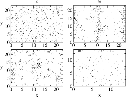
Figure 1: Spatial distribution of particles in the steady state, when the inertia is irrelevant (or almost), $\tau<T$. a) Case with no collisions. $T=10$, $\alpha=10$ ($\tau_{f}\approx 2$), and $\tau=0.1$. The number of particles is $N=500$ and the final time $500$. b) Same as before but with almost elastic collisions and $\tau_{c}<<\tau_{f}$. Here $r=0.99$, $\tau_{c}=0.01$, $\tau_{f}\approx 2$. c) Same as before but with inelastic collisions, $r=0.6$. d) Also the case of inelastic collisions, but now $\tau_{f}<<\tau_{c}$. The number of particles is $N=200$ and $T=0.2$, $\alpha=1$ ($\tau_{f}\approx 0.08$), $\tau=0.2$, $\tau_{c}=0.1$, and $r=0.1$. Final time also $500$ units.

First we consider the case of irrelevant inertia, $\tau<<T$. Obviously, in the absence of collisions, particles follow strictly the fluid and no aggregation appears (see Fig. 1a)). In fact, $\tau$ is the relaxation time of the particles to the driving flow; without collisions the particles are continuously flowing through the entire spatial domain since no KAM tori are present in the flow. However, everything changes when the collisions are taken into account. Thus, if $\tau_{c}<\tau$, the last term in Eq. (3) is the most relevant one. If we have also that $\tau_{c}<\tau_{f}$ an aggregation of the particles is always observed for any value of $r$ (even, and most noticeably, at $r=1$). This can be understood from Eq. (3), since now the velocity of the particles can be written as:

$$\hat{\bf v}\approx\hat{\bf u}+\frac{\tau}{\tau_{c}}\bf F_{col}.$$ (6)

Thus, the effect of collisions is similar to that of inertia when considered alone: the velocity of the particles is modified respect to that of the fluid parcels, then it is no longer compressible ($\bf\nabla\cdot\hat{\bf v}\neq 0$), and there are regions where particles aggregate. Figs. 1b) and 1c) show a pattern of the distribution of particles for $r=0.99$ and $r=0.6$, respectively. It is also very important to note here a specific behavior of elastic or quasi-elastic collisions ($r\approx 1$). The effect of multiple elastic collisions is equivalent to macroscopic diffusion, which, if large enough, may induce a dispersing mechanism that prevents clustering. Summing up, one can say that elastic collisions induce a clustering inertia-like effect, that disappears when diffusion is strong enough. Quantitatively this is controlled by the adimensional parameter $\tau/\tau_{c}$ since the macroscopic diffusivity $D\propto 1/\tau_{c}$. Increasing $\tau/\tau_{c}$ clustering like that of Fig. 1b) disappears and a homogeneous distribution is attained (see discussion below on the $P(m)$ function and Fig. 2a)).

On the contrary, when $\tau_{f}<\tau_{c}$ (and also $\tau_{c}<<\tau$) the strong chaoticity of the flow dominates and avoids the formation of any clustering in the system, see Fig. 1d). Finally, it is obvious from Eq.(3) that the limit $\tau<<\tau_{c}$ is equivalent to the absence of collisions, thus no clusterization appears.

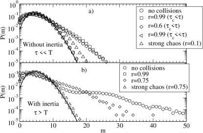
Figure 2: Distribution of clusters for the same cases shown in figure 1 (above) and 3 (below). Solid line is the analytical Poisson distribution.

A more quantitative analysis of clustering follows. This is performed via a particle-in-cell histogram, i.e., after dividing the system in $M$ small boxes (we use $N/M=5$) an histogram is made with the number of boxes containing $m$ particles, denoted the corresponding function as $P(m)$. For an homogeneous system of particles $P(m)$ is a Poisson distribution $exp(-\lambda)\lambda^{m}/m!$, where $\lambda=N/M$. As the clustering is stronger developed, the deviations from a Poissonian are more evident. Fig. 2a) calculates $P(m)$ for the patterns shown in Fig. 1, and one more case. We observe the appearance of clustering for $r<1$, and even for $r\approx 1$. Also, it is shown how for the elastic case the Poisson distribution is approached when $\tau/\tau_{c}<<1$.

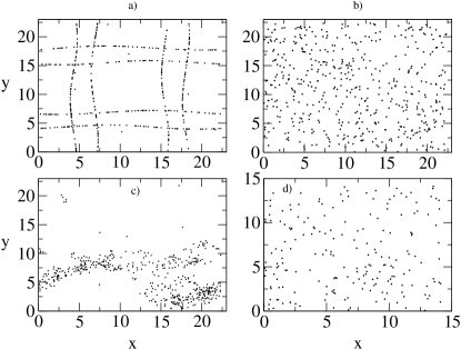
Figure 3: Spatial distribution of particles in the steady state, when the inertia is relevant, $\tau>T$. a) Corresponds to the case without collisions. Here $T=1$, $\alpha=0.5$, and $\tau=10$. The number of particles is $N=500$ and the final time $500$. b) Same as before but now with almost elastic collisions, with $\tau_{c}<<\tau_{f}$. Here $r=0.99$, $\tau_{c}=0.1$, $\tau_{f}\approx 1$. c) Same as before but with inelastic collisions, $r=0.75$ (here the final time is $175$ as the program breaks because of collapse earlier. d) Also the case of inelastic collisions, but now $\tau_{f}<<\tau_{c}$. The number of particles is $N=200$ and $T=0.2$, $\alpha=1$ ($\tau_{f}\approx 0.08$), $\tau=2$, $\tau_{c}=0.2$, and $r=0.75$. Final time also $500$ units.

It is very relevant to know the effect of collisions in the context of transport of inertial particles in chaotic flows. Therefore, we next consider the general case where the inertial term is relevant, $\tau>T$ (but otherwise $\tau$ small enough such that the l.h.s is not negligible with respect to first term in the r.h.s). It is well-known gen:tur that, in the absence of collisions, heavy particles accumulate in regions of low strain and high vorticity, the so-called preferential concentration phenomenon. In our case, the clustering steady pattern is shown in Fig. 3a). After including collisions one has: if $\tau<<\tau_{c}$ no effect is observed as the last term in the r.h.s of Eq. (3) can be neglected. A different behavior is observed when $\tau_{c}<<\tau$. Regardless of the value of $\tau_{f}$, in the limit of elastic collisions ($r\approx 1$) no aggregation of the particles is observed, Fig. 3b). As explained before, when $\tau/\tau_{c}$ is large, the continuous elastic colliding processes of the particles induce a diffusive effect that prevents clustering. On the contrary, as we go into the inelastic regime, $r<1$, the chaotic time scale, $\tau_{f}$, now plays a very important role. Thus, when $\tau_{c}<\tau_{f}$ particles aggregate although in a very different pattern to that obtained in the absence of collisions (Fig. 3c)). In particular, at variance with clustering in the absence of collisions (see Fig. 3a)), clusters are created and destroyed continuously, and moving with the flow. In this case, the particles aggregate thanks to the inelastic collisions and because the flow is not chaotic enough to disperse completely the clusters. The opposite is observed, Fig. 3d), when $\tau_{f}<\tau_{c}$; the clusters do not resist the dispersion of the flow and the density of particles is homogeneous. The corresponding $P(m)$ function is plotted in Fig. 2b).

For completeness, we briefly mention the limit $\tau>>T$. This is completely equivalent to a freely cooling granular gas since the external flow is irrelevant. Thus, clustering is usually observed for inelastic collisions goldhirsch .

In this letter we have studied numerically the stationary spatial structure of a granular material advected by a chaotic flow. We have seen that the relative importance of collisions, inertia and chaoticity of the flow gives rise to transitions from homogeneous to inhomogeneous density of grains. We think that our simple model is relevant for real physical phenomena that involve the transport of a large amount of heavy particles, like for example those appearing in many geophysical situations.

- (1) A. Babiano, J.H.E. Cartwright, O. Piro, and A. Provenzale, Phys. Rev. Lett. 84, 5764 (2000); T. Nishikawa, Z. Toroczkai, C. Grebogi and T. Tél, Phys. Rev. E 65, 026216 (2001).
- (2) T. Elperin, N. Kleeorin, and I. Rogachevskii, Phys. Rev. Lett. 77, 5373 (1996); E. Balkovsky, G. Falkovich, and A. Fouxon, Phys. Rev. Lett. 86, 2790 (2001); T. Elperin, N. Kleeorin, V. S. L’vov, I. Rogachevskii, and D. Sokoloff Phys. Rev. E 66, 036302 (2002).
- (3) W. Reade and L. Collins, Phys. Fluids 12, 2530 (2000).
- (4) H.M. Jaeger and S.R. Nagel, Science 255, 1523 (1992); H.M. Jaeger, S.R. Nagel and R.P. Behringer, Phys. Today April 1996; H.M. Jaeger, S.R. Nagel and R.P. Behringer, Rev. Mod. Phys. 68, 1259 (1996), and references therein.
- (5) C. S. Campbell, Annu. Rev. Fluid Mech. 22, 57 (1990).
- (6) G. Metcalfe, T. Shinbrot, J. McCarthy and J. M. Ottino, Nature 374, 39 (1995); T. Shinbrot, A.W. Alexander, and F.J. Muzzio, Nature 397, 675 (1999).
- (7) H. Aref, J. Fluid Mech. 143, 1 (1984); A. Crisanti, M. Falcioni, G. Paladin and A. Vulpiani, Riv. Nuov. Cim. 14, 1 (1991).
- (8) Granular Gases, volume 564 of Lectures Notes in Physics, T. Pöschel and S. Luding editors, Berlin Heidelberg, Springer-Verlag (2001).
- (9) A. Puglisi, V. Loreto, U. M. B. Marconi, A. Petri, and A. Vulpiani, Phys. Rev. Lett. 81, 3848 (1998).
- (10) M. Maxey and J. Riley, Phys. Fluids 26, 883 (1983); M. Maxey, J. Fluid Mech. 174, 441 (1987).
- (11) G. A. Bird, Molecular gas dynamics, Clarendon Press, Oxford, 1976.
- (12) T. Watanabe, H. Kaburaki and M. Yokokawa, Phys. Rev. E 49, 4060 (1994).
- (13) It should be noted that equations (1) represent a dissipative dynamical system, i.e. even in the case of non-interacting (or equivalently elastic) particles an attractor is always reached.
- (14) L. Berthier, J.-L. Barrat, and J. Kurchan Phys. Rev. Lett. 86, 2014 (2001).
- (15) T. H. Solomon and J. P. Gollub, Phys. Rev. A 38, 6280 (1988).
- (16) I. Goldhirsch and G. Zanetti, Phys. Rev. Lett. 70, 1619 (1993).