Forced Burgers Equation in an Unbounded Domain

Abstract

The inviscid Burgers equation with random and spatially smooth forcing is considered in the limit when the size of the system tends to infinity. For the one-dimensional problem, it is shown both theoretically and numerically that many of the features of the space-periodic case carry over to infinite domains as intermediate time asymptotics. In particular, for large time $T$ we introduce the concept of $T$-global shocks replacing the notion of main shock which was considered earlier in the periodic case (1997, E et al., Phys. Rev. Lett. 78, 1904). In the case of spatially extended systems these objects are no anymore global. They can be defined only for a given time scale and their spatial density behaves as $\rho(T)\sim T^{-2/3}$ for large $T$. The probability density function $p(A)$ of the age $A$ of shocks behaves asymptotically as $A^{-5/3}$. We also suggest a simple statistical model for the dynamics and interaction of shocks and discuss an analogy with the problem of distribution of instability islands for a simple first-order stochastic differential equation.
Key words: Burgers turbulence, stochastic forcing, shock discontinuities

I Introduction

The $d$-dimensional forced Burgers equation

$$\partial_{t}{\bm{u}}+\left({\bm{u}}\cdot\nabla\right){\bm{u}}=\nu\nabla^{2}{\bm{u}}-\nabla F({\bm{x}},t),\qquad{\bm{u}}=-\nabla\psi$$ (1)

which describes the dynamics of a stirred, pressure less and vorticity-free fluid, has found interesting applications in a wide range of non-equilibrium statistical physics problems. It arises, for instance, in cosmology where it is known as the adhesion model gss89 , in vehicular traffic css00 or in the study of directed polymers in random media bmp95 . The associated Hamilton–Jacobi equation, satisfied by the velocity potential $\psi$,

$$\partial_{t}\psi-\frac{1}{2}\left|\nabla\psi\right|^{2}=\nu\nabla^{2}\psi+F({\bm{x}},t),$$ (2)

has been frequently studied as a nonlinear model for the motion of an interface under deposition : when the forcing potential $F$ is random, delta-correlated in both space and time, Eq. (2) is the well-known Kardar–Parisi–Zhang (KPZ) equation kpz86 . The case with large-scale forcing was considered in Refs. s91 ; cy95 as a natural way to pump energy in order to maintain a statistical steady state. Burgers equation is then a simple model for studying the influence of well-understood structures (shocks, preshocks, etc) on the statistical properties of the flow. As it is well known, Eq. (1) in the limit of vanishing viscosity ($\nu\to 0$) displays after a finite time dissipative singularities, namely shocks, corresponding to discontinuities in the velocity field. In the presence of large-scale forcing, it was recently stressed for the one-dimensional case ekms97 ; ekms00 and also for higher dimensions ik01 ; bik02 , that the global topological structure of such singularities is strongly related to the boundary conditions associated to the equation. More precisely, when, for instance, space periodicity is assumed, a generic topological shock structure can be outlined. It plays an essential role in understanding the qualitative features of the statistically stationary regime.

So far, the singular structure of the forced Burgers equation was mostly investigated in the case of finite-size systems with periodic boundary conditions. It is however frequently of physical interest to investigate instances where the size of the domain is much larger than the scale, so as to examine, for example, the role of Galilean invariance p95 . The main goal of the present paper is to describe the singular structure of Burgers equation (1) in unbounded domains. To achieve this goal we consider the case of spatially periodic forcing with a forcing scale $L_{f}$ much smaller than the system size $L$. More precisely, we assume that the force is random and white in time, homogeneous, isotropic, smooth and $L$-periodic in space and investigate the limit $L/L_{f}\gg 1$, while keeping a constant injection rate of energy. Hence, for a fixed size of a system $L$ we consider a stationary regime corresponding to the limit $t\to\infty$ and then study the limit $L\to\infty$ with the ${\cal L}^{2}$ norm of the forcing growing like $L$. As we will see, most of the concepts associated to infinite time asymptotics introduced for the periodic case can be generalized in this limit as intermediate time asymptotics.

It is important to mention that the problem we are discussing has also another interpretation which has no direct relation to Burgers equation. In fact, we are studying the structure of singularities for variational problems associated to generic time-dependent Lagrangians in unbounded domains. From this point of view the random forcing is just a natural way to characterize generic time-dependence.

The paper is organized as follows. In Sec. II we give a brief exposition of the theory in the case of periodic forcing. In particular, we introduce the variational approach to Burgers turbulence and present results on the existence and the uniqueness of the main shock and the global minimizer. In Sec. III we introduce the notion of $T$-global shocks and describe their behavior in the time asymptotics $L_{f}/u_{\rm rms}\ll T\ll L/u_{\rm rms}$, where $u_{\rm rms}$ is the root-mean-square velocity. We also discuss theoretical and numerical results for the density of $T$-global shocks and the probability density function (PDF) of the age of shocks. In Sec. IV, we discuss an analogy with stability theory for one-dimensional stochastic ordinary differential equation (ODE) and present a simple statistical model for the interaction of shocks. Section V contains concluding remarks and, in particular, an interpretation of the results in terms of an inverse cascade. Most of the results of this paper are focusing on the one-dimensional case. We finish with a brief discussion of possible extensions to the multi-dimensional case.

II Periodic forcing

In the case of smooth spatially periodic forcing potential $F({\bm{x}},t)$, it was shown in the one-dimensional case ekms00 and for higher dimensions ik01 that a statistical steady state is reached at large times by the solution to the Burgers equation. Taking the initial time at $-\infty$, the velocity field is periodic in space and uniquely determined by the realization of the forcing. At an arbitrary time $t$, this unique solution can be expressed in terms of the following variational principle l57 ; o57 ; l82 involving the Lagrangian action $\cal A$ :

$${\bm{u}}({\bm{x}},t) = \nabla_{\bm{x}}\min_{{\bm{\gamma}}:{\bm{\gamma}}(t)=x}\left[{\cal A}\left(\bm{\gamma},t\right)\right],$$ (3)

$${\cal A}\left(\bm{\gamma},t\right) \equiv \int_{-\infty}^{t}\left[{1\over 2}\left|\dot{\bm{\gamma}}(\tau)\right|^{2}-F\left({\bm{\gamma}}(\tau),\tau\right)\right]d\tau.$$ (4)

The minimum in (3) is taken over all absolutely continuous curves ${\bm{\gamma}}(\tau)$ of ${\mathbb{R}}^{d}$ with $\tau\in(-\infty,t]$ such that ${\bm{\gamma}}(t)={\bm{x}}$. A curve minimizing the action in (3) is called a one-sided minimizer. It corresponds to a fluid particle trajectory which is not absorbed by shocks till time $t$. For all times $\tau<t$, such a minimizer is a trajectory of the dynamical system corresponding to the Lagrangian flow and thus satisfies the Newton equation

$$\ddot{\bm{\gamma}}(\tau)=-\nabla F({\bm{\gamma}}(\tau),\tau).$$ (5)

Since the force is potential and spatially periodic, the mean velocity

$$\bm{b}\equiv\frac{1}{L^{d}}\int_{[0,L]^{d}}\bm{u}({\bm{x}},t)d{\bm{x}}$$ (6)

is the first integral of (1). When the initial time is taken at $-\infty$, so that the statistically stationary regime is reached, the mean velocity $\bm{b}$ is the only information remaining from the initial condition. For simplicity, we consider in the sequel the case of a vanishing mean velocity ($\bm{b}=0$), but all the results remain true for arbitrary $\bm{b}$.

It is easy to show that for Lebesgue almost all $\bm{x}$ there exists a unique one-sided minimizer. The locations where there are more than one minimizer correspond to shock positions. Those are exactly the positions where the velocity potential $\psi({\bm{x}},t)$, which is a Lipschitz function, is not differentiable, so that the piecewise continuous velocity field ${\bm{u}}({\bm{x}},t)=-\nabla\psi({\bm{x}},t)$ has jump discontinuities. As $t\to-\infty$, all the one-sided minimizers which originated at time $t$ converge backward-in-time to the trajectory of the unique fluid particle which is never absorbed by a shock. This trajectory, denoted $\bm{\gamma}_{\rm gm}(\cdot)$, is called the global minimizer because it is an action-minimizing trajectory at any time. The statement about uniqueness of the global minimizer holds under some natural conditions on the forcing potential (see, e.g., Refs. ekms00 ; ik01 ). Shocks are generically born at some finite time and then grow and merge. There exist a particular shock structure, called the main shock ($d=1$) or the topological shock ($d>1$) which has always existed in the past. This shock can be constructed by unwrapping the picture to the whole space ${\mathbb{R}}^{d}$ (see Fig. 1 for the case $d=1$). We then obtain a lattice of periodic boxes, each of them containing a periodic image of the global minimizer and the topological shock corresponds to the set of ${\bm{x}}$-positions giving rise to several minimizers that approach different global minimizers belonging to different images of the periodic box.

Figure 1: Sketch of the unwrapped picture in space-time for $d=1$; each minimizer converges backward in time to one of the periodic image of the global minimizer. The main shock is defined as the location from which emanate two minimizers approaching different images of the global minimizer.

We focus now on the one-dimensional case with a space-periodic forcing potential of period $L$. In this case, the global minimizer is a hyperbolic trajectory of (5) and is thus associated to a smooth unstable manifold which is a smooth curve in the position-velocity phase-space $(x,u)$. The main shock is defined as the unique position giving rise to the left-most and the right-most one-sided minimizers approaching the global one backward-in-time. By definition, the trajectory of the global minimizer $\gamma_{\rm gm}(t)$ and the main shock trajectory $X_{\rm ms}(t)$ never intersect, so that they have to satisfy $X_{\rm ms}(t)<\gamma_{\rm gm}(t)<X_{\rm ms}(t)+L$. Hence, the large-scale displacement of the two-sided minimizer is the same as for the main shock. The Lagrangian flow (5) is a second-order stochastic ODE. Assuming the vanishing of the mean velocity $b$, one may be tempted to think that the displacement of a typical trajectory $\gamma(t)$ scales like the integral of the Brownian motion :

$$\left\langle\left(\gamma(t)-\gamma(0)\right)^{2}\right\rangle\propto|t|^{3}\quad\mbox{when }|t|\to\infty.$$ (7)

However this scaling does not apply to the minimizers because the particularity of such trajectories cannot be ignored. Indeed, when investigating the typical displacement of the global minimizer, we find that

$$\left\langle\left(\gamma_{\rm gm}(t)-\gamma_{\rm gm}(0)\right)^{2}\right\rangle\propto|t|\quad\mbox{when }|t|\to\infty.$$ (8)

This result was obtained by numerical study of the behavior at large times of the position of the main shock. This gives the large-time typical displacement of the position of the main shock which, as we have seen above, coincides up to a constant with the displacement of the global minimizer.

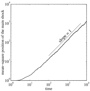
Figure 2: Average over 500 realizations of the position $X(t)$ of the main shock as a function of time for $b=0$ and a space-periodic forcing with period $L=L_{f}$.

For the numerical investigation, we chose a forcing which is the sum of independent random impulses acting at discrete “kicking” times bfk00 . Between successive kicks, the solution to the Burgers equation decays. This method is particularly efficient for obtaining the solution in the limit of vanishing viscosity, as one can use between kicks the fast Legendre transform method nv94 which is directly connected with the variational principle (3) and the Lagrangian picture of the flow. The position of the main shock is obtained by a Lagrangian method which is based on the analysis of the right-most and the left-most positions from which the two-sided minimizer is approached. Figure 2 shows the diffusive-like behavior of the main shock trajectory for a Gaussian forcing confined to the first three Fourier modes in the case when the mean velocity $b$ vanishes.

The diffusive behavior of the global minimizer has also a simple theoretical explanation. Indeed, the mean square displacement of the global minimizer can be expressed through its velocity as

$$\left\langle\left(\gamma_{\rm gm}(t)-\gamma_{\rm gm}(0)\right)^{2}\right\rangle=\left\langle\left(\int_{0}^{t}\dot{\gamma}_{\rm gm}(s)\,ds\right)^{2}\right\rangle,$$ (9)

where the velocity of the global minimizer $\dot{\gamma}_{\rm gm}(s)$ is a stationary random process. The hyperbolicity of the global minimizer implies that the time correlations for this process decay exponentially. Hence, there are just two possibilities: the mean-square displacement (9) either grows linearly with time, which gives (8), or it stays bounded in a limit $t\to\infty$. The latter behavior can be easily ruled out since the trajectory of the global minimizer does fluctuate.

III Statistics of $T$-scales in large-size systems and PDF for the age of shocks.

As we have discussed above, the existence of the main shock in the spatially periodic situation follows from a simple topological argument. The main shock is unique when the system is considered on the torus corresponding to its period (circle for $d=1$). However, if the system is considered on the whole real line (universal cover), then there exists, at each moment of time, an $L$-periodic one-dimensional lattice of main shocks. Each of these shocks is associated to two minimizers (left-most and right-most) which also form a periodic structure. In the case of the main shocks the distance between these two minimizers tends to $L$ as $t\to-\infty$. For all other shocks the corresponding distance tends to 0. In this sense, the main shocks are the only global shocks present in the system. There is also another way to characterize the main shock. Namely, the main shock is the only shock which existed forever in the past, that is, the main shock is infinitely old, contrary to all other (local) shocks, all of them being created at a finite time and hence having a finite age. In other words, local shocks can be traced backward in time only for a certain finite interval of time. The length of this time interval is what we call the age $A$ of the shock.

When we drop the periodicity condition and consider large-size systems, the main shock disappears. But one can still introduce the notion of $T$-global shocks, that is shocks which behave like the main shock when observed during a time scale of the order of $T$. As in the case of periodic boundary conditions, there are now also two equivalent ways to characterize $T$-global shock. Geometrically, one can again consider left-most and right-most minimizers associated to a given shock. After tracing them backward in time for time intervals longer than a certain “correlation time”, these two minimizers are getting close and start converging to each other exponentially fast. $T$-global shocks are defined as shocks for which this “correlation time” is larger than $T$. This means that for backward times $t\ll T$, one has $d(t)\gtrsim L_{f}$, where $d(t)$ is the distance between minimizers. Equivalently, one can say that $T$-global shocks have a finite age larger than $T$. Below, we study the statistics of the $T$-global shocks.

We start with a numerical investigation of the forced Burgers equation in a domain of a size $L$, much larger than the forcing length-scale $L_{f}$. The force is taken to be Gaussian, statistically homogeneous, white-noise in time and characterized by its covariance

$$\langle f(x+\ell,t+\tau)f(x,t)\rangle=B(\ell)\,\delta(\tau),$$ (10)

where $B$ is a smooth, $L$-periodic function. $L_{f}$ is the correlation length, chosen such that $B(\ell)$ is concentrated at scales $\ell<L_{f}\ll L$. The injection rate of energy per unit length is kept constant (i.e. we choose the space correlation such that $B(0)\propto L$). Such a hypothesis is essential because we found that it prevents any $L$ dependency of the root-mean-square velocity $u_{\rm rms}\equiv\left\langle u^{2}(x,t)\right\rangle^{1/2}$. We will now study the behavior of the statistically stationary solution for the intermediate time asymptotics $L_{f}/u_{\rm rms}\ll t\ll L/u_{\rm rms}$. For very large but finite $L$, the problem is well-defined and we can suppose that the initial condition is taken at $-\infty$, so that a statistical steady state is achieved for the solution of the Burgers equation.

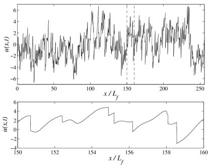
(a)

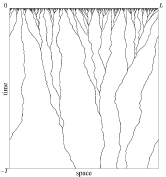
(b)

Figure 3: (a) Upper: snapshot of the velocity field for $L=256L_{f}$. Lower: zoom of the field in an interval of length $10L_{f}$, represented by dashed lines in the upper figure. (b) Minimizing trajectories in space time for the solution to the randomly forced Burgers equation periodic in space with period $L=256L_{f}$ and over a time interval of length $T=100$. The various trajectories are chosen sufficiently separated at time $t=0$ in order to lighten the picture. The minimizers converge to each other in a rather nonuniform manner, giving rise to a tree-like structure in space-time.

In order to obtain a sketch of the behavior of the solution, the limit of infinite aspect ratios $L/L_{f}$ is investigated numerically using a kicked forcing and the fast Legendre transform method (see Sec. II). Moreover, we consider here the case of a forcing whose spectrum is concentrated in the wavenumber intervals $|k|\in[\pi L_{f}/L,\,3\pi L_{f}/L]$. As we will see in Sec. V, the functional form of the forcing space correlation $B(\ell)$ at large scale $\ell\gg L_{f}$ plays an important role. Numerical observations suggest that, at any time in the statistical steady state (obtained after sufficiently long integration), the shape of the velocity profile is locally similar to the order-unity aspect ratio problem, duplicated over independent intervals of size $L_{f}$ (see Fig. 3(a)). More particularly, when tracking the trajectories of fluid particles backward in time, one can see that the convergence of the minimizers to each other is far from uniform. Figure 3(b) shows that the minimizers are forming different branches which are converging to each other backward in time, defining in space time a tree-like structure. Eventually, the number of branches decreases and a unique trunk emerges around the global minimizer. Note that the same type of behavior is also observed for shocks (see Fig. 4(a)) by running forward in time. The intermediate time asymptotics correspond to the time scale for which there is still a large number of such branches.

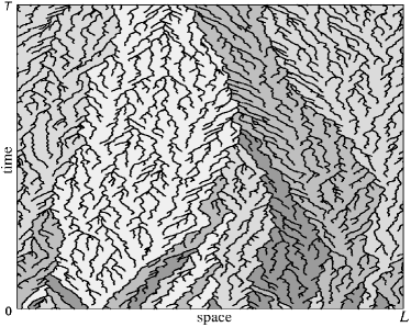
(a)

(b)

Figure 4: (a) Shock trajectories for aspect ratio $L/L_{f}=32$ and with $T=10$; the different gray areas correspond to the space-time domains associated to the different smooth pieces $\Omega_{j}$’s of the velocity field at time $t=0$. (b) Sketch of the space-time evolution of a given smooth piece $\Omega_{j}$ located between two shock trajectories $X_{1}(t)$ and $X_{2}(t)$ which merge at time $T_{j}$. The trajectories of some fluid particles are represented; the shock trajectories are represented as bold lines; the dashed curve represents the trajectory of the unique fluid particle that is simultaneously absorbed by both shocks $X_{1}$ and $X_{2}$ at the time of their merger. This trajectory is a $T$-global minimizer if $T_{j}>T$.

The velocity field at a given time, taken for convenience to be $t=0$, consists of smooth pieces separated by shocks. Let us denote by $\{\Omega_{j}\}$ the set of intervals in $[0,L)$, on which the solution $u(\cdot,0)$ is smooth. The boundaries of the $\Omega_{j}$’s are the shock positions. Each of these shocks is associated to a root-like structure formed by the trajectories of the various shocks which have merged at times $t<0$ to form the shock under consideration (see Fig. 4(a)). This root-like structure contains the whole history of the shock and in particular its age. Indeed, if the root has a finite depth, the shock under consideration has only existed for a finite time. A $T$-global shock is defined as a shock whose associated root is deeper than $-T$. One can give the dual definition for $T$-global minimizers. All the smoothness intervals $\Omega_{j}$ defined above, except that which contains the global minimizer, will be entirely absorbed by shocks after a finite time (see Fig. 4(b)). For each of these pieces, one can define a life-time $T_{j}$ as the time when the last fluid particle contained in this piece at time $t=0$ enters a shock. It corresponds to the first time for which the shock located on the left of this smooth interval at time $t=0$ merges with the shock located on the right. When the life-time of such an interval exceeds $T$, the trajectory of this latter fluid particle is called a $T$-global minimizer.

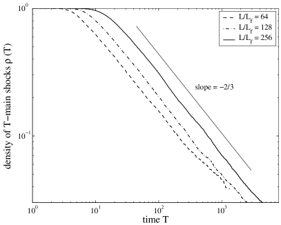
Figure 5: Density of $T$-global shocks as a function of $T$ for three different system sizes $L/L_{f}=64$, $128$ and $256$; average over 100 realizations.

Hence, for any age $T$, one can define a set of $T$-scale objects in the spatial domain $[0,L)$ at a given time $t$. We define their spatial density as the number of such objects divided by the size of the domain $L$. The density $\rho(T)$ of $T$-global shocks is investigated numerically in the kicked case by using a two-step method. Firstly, the simulation is run up to some large time $t$ for which the statistically stationary regime is reached; secondly, each shock present at time $t$ is tracked backward in time down to the instant of its creation, giving an easy way to determine the density $\rho(T)$. We also average numerical results with respect to the forcing realizations. It can be seen from Fig. 5, on which the density for three different aspect ratios $L=/L_{f}$ is presented, that the behavior of $\rho(T)$ is independent of $L$, and that it displays a power-law $\rho(T)\propto T^{-2/3}$ in the intermediate asymptotic range $L_{f}/u_{\rm rms}\ll T\ll L/u_{\rm rms}$.

We now present a simple phenomenological argument to explain the scaling exponent $2/3$. Consider the solution at a given time ($t=0$, for instance). Denote by $\ell(T)$ the typical spatial separation scale for two nearest $T$-global shocks. Obviously, $\ell(T)\sim 1/{\rho(T)}$. The mean velocity of a spatial segment of length $\ell$ is given by

$$b_{\ell}=\frac{1}{\ell}\int_{[y,\,y+\ell]}u(x,\,0)\,dx$$ (11)

Since the expected value $\left\langle u(x,\,0)\right\rangle=0$ it is natural to assume that for large $\ell$ one has the following asymptotics

$$\int_{[y,\,y+\ell]}u(x,\,0)\,dx\sim\sqrt{\ell},$$ (12)

which gives $b_{\ell}\sim\ell^{-1/2}$ for the mean velocity fluctuations. Consider now the rightmost minimizer corresponding to the left $T$-global shock and the leftmost minimizer related to the right one. Since there are no $T$-global shocks in between, it follows that the two minimizers we selected approach each other backward in time for times of the order of $-T$. This means that the backward-in-time displacement of a spatial segment of length $O(\ell)$ is itself $O(\ell)$ for time intervals of the order of $T$. The corresponding displacement is given as the sum of two competing effects: the first, a kind of drift induced by the local mean velocity $b_{\ell}$, is connected with the mean velocity fluctuations and gives a displacement $\propto b_{\ell}T$; the second effect is a standard diffusive contribution $\propto T^{1/2}$ related to the diffusive behavior of the minimizing trajectories. Taking both into account, we get

$$\ell\sim C_{1}T\ell^{-1/2}+C_{2}T^{1/2},$$ (13)

where $C_{1}$ and $C_{2}$ are numerical constants. It is easy to see that the dominant contribution comes from the first term. Indeed, if the second term dominates, i.e. $\ell\propto T^{1/2}$, the first term then gives a contribution of the order of $\ell^{3/2}$ which contradicts to (13). Hence, one should have $\ell\sim C_{1}T\ell^{-1/2}$, leading to the scaling behavior

$$\ell(T)\propto T^{2/3},\qquad\rho(T)\propto T^{-2/3}.$$ (14)

As we have already discussed above, $T$-global shocks are shocks older than $T$. Denote by $p(A)$ the PDF for the age of shocks. More precisely, $p(A)$ is a density in the stationary regime of a probability distribution of the age $A(t)$ of a shock, say the nearest to the origin. It follows from (14) that the probability of shocks whose age is larger than $A$ decays like $A^{-2/3}$, which implies the following asymptotics for the PDF $p(A)$:

$$p(A)\propto A^{-5/3}.$$ (15)

IV Two related statistical models

We next discuss a very close analogy between the problem just considered and the dynamical behavior of a simple first-order stochastic ODE. Consider the following one-dimensional stochastic Ito equation:

$$dX=f(X)\,dW(t),$$ (16)

where $0<C_{1}\leq f(x)\leq C_{2}<\infty$, $x\in{\mathbb{R}}$. We are interested in the stochastic flow generated by (16). In other words, the aim is to understand the dynamical properties in the large-time asymptotics of the trajectories corresponding to the solutions of (16) for different initial values. Let $X_{1}(t)$ and $X_{2}(t)$ with $t\geq 0$ be the two solutions associated to the initial values $X_{1}(0)=x_{1}$ and $X_{2}(0)=x_{2}$. It is well-known that the difference $[X_{1}(t)-X_{2}(t)]$ is a martingale which does not change its sign; this implies that the limit

$$c(x_{1},x_{2})\equiv\lim_{t\to\infty}\left[X_{1}(t)-X_{2}(t)\right]$$ (17)

exists and is finite.

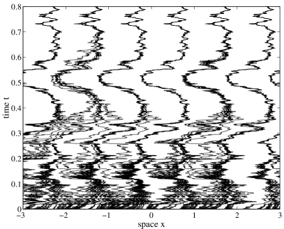
(a)

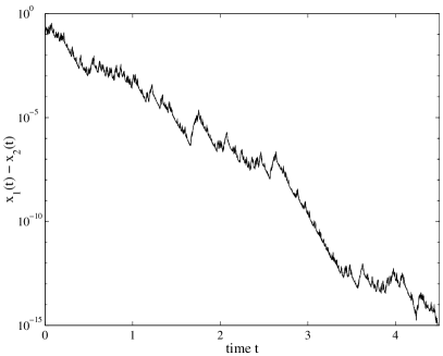
(b)

Figure 6: Behavior of the solutions to the stochastic ODE (16) for the periodic function $f(x)=2+\sin x$. (a) Unwrapped trajectories of the solutions converging to one of the periodic image. (b) Time behavior, for a given realization, of the separation between two trajectories $x_{1}(t)$ and $x_{2}(t)$ associated to two different initial conditions. The two trajectories approach each other exponentially fast with a non-random rate $\lambda$.

Consider first the case when $f(x)$ is periodic. It is easy to see that $c(x_{1},x_{2})$ has to be equal to a period of the function $f(x)$ (see, e.g., Fig. 6(a)). Let, for simplicity, the smallest period of $f(x)$ be equal to 1. Then, $c(x_{1},x_{2})$ can take only two values: either 0 or 1. In fact, it is possible to show (see Bax1 ; Bax2 ; Bax3 ; Cal ) that the following picture holds. There exists a random periodic sequence of points $x(k)=x_{*}(\omega)+k$, $k\in{\mathbb{Z}}$, $x_{*}\in[0,1)$ such that $c(x_{1},x_{2})=0$ for all $x_{1},x_{2}\in(x_{*}(\omega)+k,\,x_{*}(\omega)+k+1)$ and $c(x_{1},x_{2})=1$ for $x_{1}\in(x_{*}(\omega)+k-1,\,x_{*}(\omega)+k)$ and $x_{2}\in(x_{*}(\omega)+k,\,x_{*}(\omega)+k+1)$. Moreover, in both cases, the convergence is exponential:

$$\left|c(x_{1},x_{2})-\left(X_{1}(t)-X_{2}(t)\right)\right|\sim C\exp(-\lambda t),$$ (18)

where $\lambda>0$ is a non-random Lyapunov exponent (see Fig. 6(b)). The random variable $x_{*}(\omega)$ which determines the positions of the separation points $x(k)$ depends on the realization $\omega$ of the white noise $dW(t)$. If we consider the stochastic flow on the unit circle, then all the trajectories are stable except the one originating from $x_{*}(\omega)$. The stability is governed by the non-random positive Lyapunov exponent $\lambda$. In contrast, the trajectory which starts at $x_{*}(\omega)$ is unstable and pushes nearby trajectories away. Hence, $x_{*}(\omega)$ plays a role similar to that of the global minimizer for the Burgers equation with a spatially periodic force. An exponentially small neighborhood of it gets mapped into the whole unit circle apart from another exponentially small interval which is the image of the rest of the circle. This instability island around $x_{*}(\omega)$ is similar to the interval of fluid particles which are not absorbed by shocks until time $t$.

All the results above in the case of periodic $f(x)$ have been well-known for about 20 years and were presented here just to emphasize an analogy with the main shocks and minimizers for Burgers equation in a periodic situation. At the same time, the dynamical behavior in the non-periodic case is more complicated and much less studied. As we explain below, this behavior is also very similar to the dynamical picture governed by the repelling $T$-global shocks in the case of non-periodic Burgers equation. Since $f(x)$ is non-periodic $c(x_{1},x_{2})=0$ and all trajectories are asymptotic to each other as $t\to\infty$. However, as in the case of non-periodic Burgers equation, this convergence is very non-uniform. Although there are no globally unstable positions like $x(k)=x_{*}(\omega)+k$, for a given time scale $T\gg 1$, one still has exponentially small $T$-instability islands which separate different intervals of stability from each other. For a given time $T$, the image under the stochastic flow of the $T$-instability islands covers almost all the real line apart from exponentially small pieces which are images of the stability intervals. Those exponentially small pieces, which we call $T$-stability intervals play a role similar to that of the $T$-global shocks in Burgers turbulence. For a larger time scale $T_{1}\gg T$ a majority of $T$-instability island will become stable, while some of them will still be unstable. Those islands are in fact $T_{1}$-unstable. One can ask the same question as studied above about the asymptotics of the density of $T$-instability islands in the limit as $T\to\infty$. Our preliminary numerical results indicate that the density of $T$-instability islands scales as $T^{-1/2}$. Notice that this scaling is different from the scaling $T^{-2/3}$ in the case of Burgers equation. We believe that in the case of a stochastic flow the $T$-instability islands and the density of them can be defined and studied rigorously. The simplification is connected with the absence of a slow drift which one has for Burgers equation due to fluctuations of the average velocity. In the case of the stochastic flow the whole asymptotic dynamical picture is formed by just two factors: diffusion and hyperbolic contraction. As a result, the rigorous analysis of the model seems to be a realistic task.

We finally suggest a simple statistical model which captures the essential characteristics of the dynamics and the interactions of $T$-global shocks and $T$-stability intervals. We believe that this model is also quite interesting on its own. Consider an infinite system of particles on a one-dimensional integer lattice ${\mathbb{Z}}$. Two different particles cannot occupy the same site, and some sites are in general not occupied. Each particle is associated to an integer age $A\geq 0$. The model consists in describing a discrete time evolution of particles. To get a configuration of particles at the next step, we proceed as follows. First of all, with a probability $0<p<1$, we generate independently new particles in every non-occupied site and we set the age $A=0$ for all newly born particles. Then, each particle independently jumps, with a probability $1/2$, either to the right or to the left by a distance $1/2$ and we add $1$ to the age of all particles. Notice that, after one time step, the particles are located on the sites of the dual lattice. If there are two particles which jumped into the same point of the dual lattice, we then assume that the older one absorbs the younger, that is we ascribe to this site a particle whose age is the maximum of the two ages of the merging particles. It is easy to see that this dynamics reaches a statistical steady state and one can define an integer-valued random variable $A$ which is the age of the particle closest to the origin, say from the right. The probability distribution of this random variable, namely the asymptotics as $A\to\infty$ of the probability $p(A)$, is closely connected with the statistics of $T$-instability intervals for the non-periodic stochastic flow which we discussed above. A numerical study of the model suggests that $p(A)$ scales like $A^{-3/2}$ which corresponds to the scaling $T^{-1/2}$ for the density of $T$-instability islands. We postpone the detailed numerical and theoretical analysis of the non-periodic stochastic flow and the statistical model of interacting particles until a future publication.

V Concluding remarks

We have studied the inviscid randomly forced Burgers equation with non-periodic forcing on the whole real line started at $t=-\infty$. Our results indicate the existence of stationary regime which corresponds to the velocities of one-sided minimizers and suggest the following picture. At any given time $t$ (say $t=0$) and any given $x\in{\mathbb{R}}$, there exists at least one one-sided minimizer. However, due to fluctuations of the positions of one-sided minimizers, there are no global minimizers. This means that any fluid particle gets absorbed by a shock after a certain time. Any two one-sided minimizers are asymptotic to each other backwards-in-time, that is the distance between them tends to zero as $t$ tends to $-\infty$. However, this convergence is very nonuniform. For fixed $x,y\in{\mathbb{R}}$ one-sided minimizers which originated at $t=0$ in $x$ and $y$ will approach each other exponentially fast beyond a certain correlation time $T(x,y)$. This correlation time is of the order of the maximum $T$ for which a $T$-global shock exists between $x$ and $y$. One can say that $T$-global shocks form a hierarchical structure separating different stability domains from each other. By stability domains we understand intervals for which one-sided minimizers converge exponentially fast with a correlation time of the order of the turnover time $L_{f}/u_{\rm rms}$. The separation by $T$-global shocks form separation “walls” between these different stability intervals for times of the order of $-T$. For larger backward times, one-sided minimizers from the neighboring stability intervals are exponentially asymptotic to each other. Another interpretation of $T$-global shocks is connected with their time of creation. Every shock can be traced backward only for a finite time interval. For $T$-global shocks, this time interval which determines the age of the shock is larger than $T$. Since all shocks have a finite age, it follows that there are no true main shocks in the non-periodic situation. Our results suggest that the large-$T$ asymptotics of the density of $T$-global shocks follows the power-law $\rho(T)\propto T^{-2/3}$. This gives a power-law behavior with exponent ${5}/{3}$ for the PDF of the age of shocks: $p(A)\propto A^{-5/3}$. Another related exponent is connected with the absorption times, defined in the following way. The absorption time $T(\ell)$ is the time after which all fluid particles in the spatial interval $[-\ell/2,\,\ell/2]$ are absorbed by shocks. Using the duality between the forward-in-time behavior of fluid particles (minimizers) and the backward-in-time behavior of shocks, we find that the absorption times $T(\ell)\propto\ell^{3/2}$ at large $\ell$.

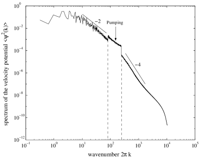
Figure 7: Spectrum $\langle\hat{\psi}^{2}(k)\rangle$ of the velocity potential in the stationary regime for the aspect ratio $L/L_{f}=128$. This spectrum contains two power-law ranges: at wavenumbers $k\gg L/L_{f}$, the traditional $\propto k^{-4}$ inertial range connected to the presence of shocks in the solution and, for $k\ll L/L_{f}$, an “inverse cascade” $\propto k^{-2}$ associated to the large-scale fluctuations of $\psi$

Notice that the power-law behavior of the density $\rho(T)$ of $T$-global shocks can be interpreted in term of a kind of inverse cascade in the spectrum of the solution (although there is no conserved energy-like quantity). Indeed, the fluctuations (12) of the mean velocity suggest that, for large-enough separations $\ell$, the velocity potential increment scales like

$$\left|\psi(x+\ell,\,t)-\psi(x,\,t)\right|\propto\ell^{1/2}.$$ (19)

This behavior is responsible for the presence of an intermediate power-law range with exponent $-2$ in the spectrum of the velocity potential at wavenumbers smaller than the forcing scale (see Fig. 7). This power-law range corresponds for the velocity spectrum to an equipartition of kinetic energy, meaning that the large-domain asymptotics may be considered in the same universality class as the KPZ problem for interface dynamics. It is also important to notice that, in order to obtain this $-2$ range at small wavenumbers, the spectrum of the forcing potential must go to zero faster than $k^{-2}$ as $k\to 0$. Otherwise, the leading behavior is non-universal and depends on the functional form of the forcing correlation.

The randomly forced Burgers equation in an unbounded domain with a different type of forcing was also considered in Ref. hk02 , where it was assumed that the forcing potential has at any time its global maximum and its global minimum in a prescribed compact part of the space. Such a forcing leads to a completely different behavior. In particular, in this case there exists a global minimizer located in a finite spatial interval for all times and all other minimizers are asymptotic to it in the limit $t\to\infty$.

We finally stress that, in this paper, we have mostly discussed the one-dimensional case. It is of particular interest to analyze the effects of non-compactness of the domain and the intermediate time asymptotics in higher dimensions. The notion of main shock is then replaced by that of topological shock ik01 ; bik02 , which are no more isolated points, but spatially extended objects. The natural problem in this setting is to study geometrical and statistical properties of the $T$-global shocks and to find the asymptotic behavior of their age distribution.

References

- (1) S.N. Gurbatov, A.I. Saichev and S.F. Shandarin, The large-scale structure of the Universe in the frame of the model equation of non-linear diffusion, Monthly Notices of the Royal Astronomical Society 236:385–402 (1989).
- (2) D. Chowdhury, L. Santen and A. Schadschneider, Statistical physics of vehicular traffic, Phys. Rep. 329:199–329 (2000).
- (3) J.-P. Bouchaud, M. Mézard and G. Parisi, Scaling and intermittency in Burgers turbulence, Phys. Rev. E 52:3656–3674 (2000).
- (4) M. Kardar, G. Parisi and Y.-C. Zhang, Dynamic scaling of growing interfaces, Phys. Rev. Lett. 56:889–892 (1986).
- (5) Ya.G. Sinai, Two results concerning asymptotic behavior of the solutions of the Burgers equation with force, J. Stat. Phys. 64:1–12 (1991).
- (6) A. Chekhlov and V. Yakhot, Kolomogorov turbulence in a random-force-driven Burgers equation, Phys. Rev. E 51:R2739–R2742 (1995).
- (7) W. E, K. Khanin, A. Mazel and Ya.G. Sinai, Probability distribution functions for the random forced Burgers equation, Phys. Rev. Lett. 78:1904–1907 (1997).
- (8) W. E, K. Khanin, A. Mazel and Ya.G. Sinai, Invariant measures for Burgers equation with stochastic forcing, Ann. Math. 151:877–960 (2000).
- (9) R. Iturriaga and K. Khanin, Burgers turbulence and random Lagrangian systems, Comm. Math. Phys., in press (2002).
- (10) J. Bec, R. Iturriaga and K. Khanin, Topological shocks in Burgers turbulence, Phys. Rev. Lett. 89:024501 (2002).
- (11) A. Polyakov, Turbulence without pressure, Phys. Rev. E 52:6183–6188 (1995).
- (12) P.D. Lax, Hyperbolic systems of conservation laws II, Commun. Pure Appl. Math. 10:537–566 (1957).
- (13) O. Oleinik, Discontinuous solutions of nonlinear differential equations, Uspekhi Mat. Nauk 12:3–73 (1957). (Russ. Math. Survey., Am. Math. Transl. Series 2 26:95–172).
- (14) P.-L. Lions, Generalized solutions of Hamilton–Jacobi equations, Research Notes in Math. 69, Pitman Advanced Publishing Program, Boston (1982).
- (15) J. Bec, U. Frisch and K. Khanin, Kicked Burgers turbulence, J. Fluid Mech. 416:239–267 (2000).
- (16) A. Noullez and M. Vergassola, A fast Legendre transform algorithm and applications to the adhesion model, J. Sci. Comp. 9: 259–281 (1994).
- (17) P.H. Baxendale, Stability and equilibrium properties of stochastic flows of diffeomorphisms. Diffusion processes and related problems in analysis, Vol. II (Charlotte, NC, 1990), 3–35, Progr. Probab. 27, Birkhäuser Boston, Boston, MA, 1992.
- (18) P.H. Baxendale, Asymptotic behaviour of stochastic flows of diffeomorphisms. Stochastic processes and their applications (Nagoya, 1985), 1–19, Lecture Notes in Math., 1203, Springer, Berlin, 1986.
- (19) P.H. Baxendale, Asymptotic behaviour of stochastic flows of diffeomorphisms: two case studies, Probab. Theory Relat. Fields 73:51–85 (1986).
- (20) A. Carverhill, Flows of stochastic dynamical systems: ergodic theory, Stochastics 14:273–317 (1985).
- (21) H.V. Hoang and K. Khanin, Random Burgers equation and Lagrangian systems in non-compact domains, submitted to Nonlinearity (2002).