Saddle points in the chaotic analytic function and Ginibre characteristic polynomial

Abstract

Comparison is made between the distribution of saddle points in the chaotic analytic function and in the characteristic polynomials of the Ginibre ensemble. Realising the logarithmic derivative of these infinite polynomials as the electric field of a distribution of coulombic charges at the zeros, a simple mean-field electrostatic argument shows that the density of saddles minus zeros falls off as $\pi^{-1}|z|^{-4}$ from the origin. This behaviour is expected to be general for finite or infinite polynomials with zeros uniformly randomly distributed in the complex plane, and which repel quadratically.

It is well-known that there are several similarities between the distributions of zeros of the ensemble of random polynomials which tend to the chaotic analytic function (discussed by Hannay 1998, 1996, Bleher, Shiffman and Zelditch 2000, Forrester and Honner 1999, Leboeuf 1999, Bogomolny, Bohigas and Leboeuf 1996) and the eigenvalues of Ginibre matrices (Ginibre 1965, Mehta 1991 chapter 15), both in the finite and infinite cases. To be more precise, for $N$ large and possibly $\infty,$ we compare the zeros of the chaotic analytic function polynomials (caf polynomials)

$$f_{N,{\rm caf}}(z)=\sum_{n=0}^{N}\frac{a_{n}z^{n}}{\sqrt{n!}},$$ (1)

where the $a_{n}$ are independent identically distributed complex circular gaussian random variables, with the eigenvalues of matrices in the Ginibre ensemble, defined to be $N\times N$ matrices with entries independent identically distributed complex circular gaussian random variables. The Ginibre analogue to equation (1) is the characteristic polynomial $f_{N,{\rm Gin}}(z).$ The zeros of the two $f_{N}$ share the following properties, as discussed in the above references:

• they are uniformly randomly distributed, with density $\sigma=1/\pi,$ within a disk centred on the origin of the complex plane, which has radius $\sqrt{N},$ and smoothed boundary (Ginibre with gaussian tail outside, caf with power law);

• within this disk, the distribution of zeros is statistically invariant to translation and rotation;

• the statistical properties of the zeros at a fixed radius $r$ do not change as $N$ increases, provided that $\sqrt{N}\gtrsim r+\mathcal{O}(1);$

• the two-point correlation functions $g_{{\rm caf}},g_{{\rm Gin}}$ for zeros separated by distance $|z_{1}-z_{2}|=r\lesssim\sqrt{N}-\mathcal{O}(1)$ within the disk are given by

  $$g_{{\rm caf}}(\sqrt{2}r) = [(\sinh^{2}r^{2}+r^{4})\cosh r^{2}-2r^{2}\sinh r^{2}]/\sinh^{3}r^{2},$$ (2)

  $$g_{{\rm Gin}}(r) = 1-\exp(-r^{2}).$$ (3)

  Both of these functions exhibit quadratic repulsion at the origin, are of order 1 (uncorrelated) for $r\gtrsim 1,$ and satisfy a screening relation: the integral of $\sigma g$ over the plane, after subtracting the uniform background density, is $-1;$

• the distribution of Ginibre zeros is equivalent to a two dimensional $N$-charge Coulomb gas in a harmonic oscillator potential $|z|^{2}/2,$ at a temperature corresponding to $\beta=2,$ whereas the caf zeros have an additional $N$-body potential.

Despite these similarities, there is no obvious explicit relation between these two ensembles.

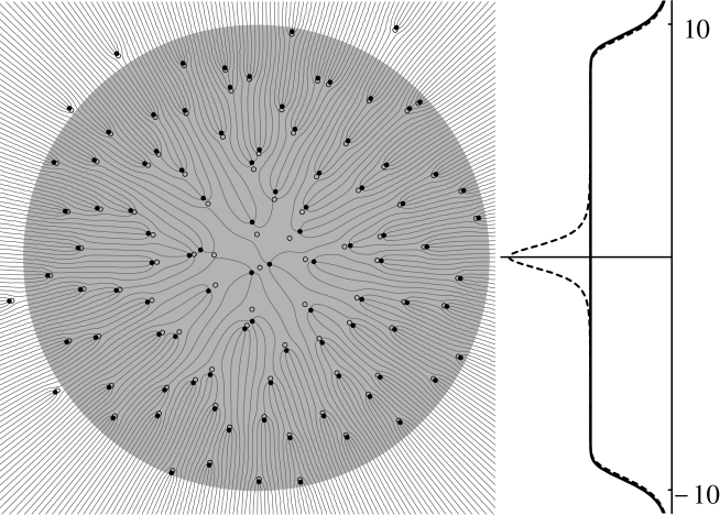
Figure 1: A sample distribution of zeros and saddles for a caf polynomial with $N=100.$ The zeros are represented by filled circles, the saddles by empty circles. The large disk has radius 10, indicating the area in which the distribution is isotropic. Lines of constant argument (equally spaced by $\pi/2$) are given by the curves; in the electrostatic analogy, they are electric field lines. The plot to the right shows the theoretical density of zeros $\sigma$ (full line) and saddles $\rho$ (dashed line) for $N=100,$ showing the saddle bump at the origin and the disk boundary smoothing (the saddle boundary lies just inside the zero boundary, giving one fewer saddles than zeros in all.

In this work, we consider the distribution of the saddle points of the polynomials $f_{{\rm caf}},f_{{\rm Gin}}$ (dropping the suffix $N$ unless necessary), that is, zeros of the derivative $\rmd f/\rmd z.$ The behaviour of the caf saddles is easy to determine, the Ginibre saddles less so. Numerical experiment shows that in both cases the saddle distribution roughly mimics the zero distribution, except for a surplus near the origin and a deficit near the disk edge. Using the electrostatic analogy, we shall see that the density of the saddles minus zeros has the same $1/\pi|z|^{4}$ tail away from the origin for each case, due to the quadratic repulsion of the zeros. Also, the cause and extent of the edge deficit will be clear.

The density of caf saddles $\rho$ can be found by replacing $f_{\rm caf}$ with $f_{\rm caf}^{\prime}$ in the formula for the density of zeros (Hannay 1996, Nonnenmacher and Voros 1998 equation (69)). When $|z|\lesssim\sqrt{N}-\mathcal{O}(1),$ the $N\to\infty$ formulae may be applied. In this case, the zero density $\sigma$ is $1/\pi$ (as mentioned above), and the saddle density is

$$\rho=\pi^{-1}\partial_{z}\partial_{z^{*}}\langle f_{{\rm caf}}^{\prime}(z)f_{{\rm caf}}^{\prime}(z)^{*}\rangle=\pi^{-1}(1+(1+|z|^{2})^{-2}).$$ (4)

This has, in addition to a uniform $1/\pi$ density, a ‘bump’ in the vicinity of the origin, which integrates to 1, and the saddle surplus is $\rho-\sigma=(\pi(1+|z|^{2})^{2})^{-1},$ which decays like $\pi^{-1}|z|^{-4}.$ For finite $N,$ of course, an order $N$ polynomial has $N-1$ saddles, not $N+1,$ implying that $\rho\approx 0$ for $|z|^{2}\gtrsim N-2,$ which is indeed the case when the calculation in equation (4) is performed for finite $N.$ The pattern of zeros and saddles for a sample caf polynomial with $N=100$ is shown in figure 1 (the pattern of Ginibre zeros and saddles look very similar), along with the corresponding plots of $\sigma$ and $\rho;$ the most obvious feature of this distribution is that zeros and saddles tend to occur in ‘bonded’ pairs, with the saddle positioned radially inwards from the zero, and the bond length decreases as $|z|$ increases. The pairing breaks down near the origin, indeed the ‘extra’ unbonded zero is in this neighbourhood.

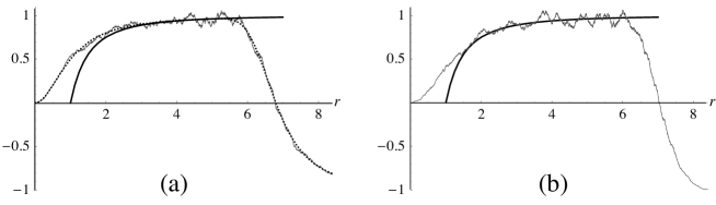
Figure 2: Plots of $\mathcal{N}(r)$ compared against the asymptotic theoretical fit: (a) caf, fitted with $1-1/r^{2}$ as in (6) (solid line) and the exact $\mathcal{N}$ from (4), (5) (dashed line); (b) Ginibre, fitted with $1-1/r^{2}$ as in (a). The data in each case are for 1000 random samples with $N=50$ (numerical errors tend to appear for Ginibre with $N$ significantly larger).

It proves to be more convenient to work with the cumulative number of saddles minus zeros within a radius $r=|z|,$ denoted by $\mathcal{N}(r),$ which is given by

$$\mathcal{N}(r) = 2\pi\int_{0}^{r}(\rho-\sigma)r^{\prime}\,\rmd r^{\prime}$$ (5)

$$\approx 1-1/r^{2}\quad\hbox{for caf, with $1\ll r\lesssim\sqrt{N}-\mathcal{O}(1).$}$$ (6)

It is our aim to show, using mean-field electrostatics, that this expression holds generally for polynomials with zeros distributed according to the bullet points above, including the Ginibre polynomials $f_{{\rm Gin}}.$ Figure 2 shows numerical plots of $\mathcal{N}(r)$ for simulations of both the caf and Ginibre polynomials, the caf fitting (6) as well as the exact theoretical curve (putting the finite form of (4) into (5)), the Ginibre, fitting with (6).

We start by recalling that the (two dimensional) electric field is represented by the logarithmic derivative of the polynomial $f,$ with $N$ zeros $z_{j},$ which electrostatically represent $N$ unit charges at positions $z_{j}$ in the plane. The logarithmic derivative $\mathcal{E}$ of $f$ is

$$\mathcal{E}(z)=\frac{\rmd\log f(z)}{\rmd z}=\sum_{j=1}^{N}\frac{1}{z-z_{j}},$$ (7)

which is Coulomb’s law in two dimensions (setting $q/2\pi\varepsilon_{0}=1$), and holds when there are arbitrarily many zeros/charges. The direction of the electric vector $\bi{E}$ is given by $\mathcal{E}^{*},$ i.e. $\bi{E}=({\rm Re}\mathcal{E},-{\rm Im}\mathcal{E}),$ and the direction of the field lines is given by the contours of constant argument of $f.$ The magnitude of the field $|\mathcal{E}|=|\bi{E}|,$ and saddles are the places where this is zero. It will also be useful to define the field due to all charges excluding a particular one at $z_{i},$

$$\mathcal{E}_{i}(z)=\sum_{j\neq i,j=1}^{N}\frac{1}{z-z_{j}}.$$ (8)

Saddles may therefore be thought of as the places where the field from a zero/charge balances the background field from all of the others. Consider a particular zero at $z_{i}$ with $\sqrt{N}-\mathcal{O}(1)\gtrsim|z_{i}|\gg 1.$ By Gauss’s law, the statistically disklike distribution of the zeros implies that the average field at $z_{i}$ due to the other charges is that due to a charge $\sigma\pi|z_{i}|^{2}$ at the origin (only zeros with modulus less than $|z_{i}|$ are relevant). This justifies electrostatically the observation from figure 1 that, for sufficiently large $z_{i},$ zeros and saddles are almost always paired, and that the saddle $s_{i}$ paired with the zero $z_{i}$ is near $z_{i},$ on the straight line between the zero and the origin. We denote the real positive ‘bond length’ $|z_{i}-s_{i}|$ by $b(s_{i})=b_{i}.$ This bond length function will be calculated below on the basis of the electrostatic model, ignoring statistical fluctuations (implying that $b(s_{i})$ is radial). This will yield $\mathcal{N}(r)$ by finding the number $\#(r)$ of bonds crossed by a circle of radius $r.$ Since for a polynomial, $\mathcal{N}(\infty)=-1$ and $\#(\infty)=0,$ we can set $\mathcal{N}(r)=\#(r)-1.$

The number $\#(r)$ is simply the number of zeros in the annulus whose inner radius $r$ is $|s_{i}|,$ and whose outer radius is $|s_{i}|+b(s_{i});$ any zero $z_{j}$ in this area will have a saddle with $|s_{j}|<|s_{i}|,$ and its bond $b_{j}$ will cross the circle of radius $|s_{i}|.$ Therefore, with $|s_{i}|=r,$ and realising that the zero density $\sigma$ is uniform,

$$\mathcal{N}(r)+1 = \#(r)=\sigma\pi[(b(r)+r)^{2}-r^{2}]$$ (9)

$$= b(r)^{2}+2rb(r).$$

The problem remains of how to calculate $b(r).$ The crudest approximation is to balance radially the field from $z_{i}$ with the field from the rest of the charges $\mathcal{E}_{i},$ again ignoring fluctuations. Using Coulomb’s law, and applying Gauss’s law at $|z_{i}|,$ gives $1/b_{i}=|z_{i}|$ or $b_{i}=1/|z_{i}|.$ Solving $b_{i}$ in terms of $|s_{i}|$ and putting into equation (9) does indeed give the required leading order terms $1-1/r^{2}$ in (6), but we have made two approximations in this argument which affect the value of $b_{i}$ at the required order. We show below that these two effects cancel each other.

The first approximation made is that Gauss’s law should really be applied at the saddle radius $|s_{i}|,$ not the zero radius $(|s_{i}|+b(s_{i})).$ Substituting this value into (9), however, gives $\mathcal{N}(r)=1+1/r^{2},$ not $1-1/r^{2}$ as desired. The second approximation is that the repulsion from $z_{i},$ embodied by the correlation function $g,$ has been neglected.

The crude approximation assumed that the field due to the charges other than $z_{i}$ to be due to a uniform jellium of density $\sigma.$ However, we know from the two-point correlation function $g$ (with the properties above) that zeros are repelled quadratically from a given one, and the background jellium is ‘dented’ around $z_{i},$ with the shape of the dent given around $z_{i}$ by $g(|z-z_{i}|).$ The correct field to use, in this case, is the mean of (8), not (7). Gauss’s law, now applied to the dent (since it is circularly symmetric around $z_{i}$), effectively weakens the field from $z_{i}.$ Including this correction as well, we have the implicit expression for $b$ (omitting $i$ subscripts):

$$\frac{1}{b}-\frac{2\pi\sigma}{b}\int_{0}^{b}(1-g(b^{\prime}))b^{\prime}\,\rmd b^{\prime}=s.$$ (10)

Since $b$ is very small (of the order of $1/s$), $g(b)$ is proportional to $b^{2}$ due to repulsion, and the $g(b^{\prime})$ part of the integrand may be neglected, integrating to $b^{2}/2$ to leading order; thus (10) implies

$$b_{i}\approx\frac{1}{|s_{i}|+b_{i}}=\frac{1}{|z_{i}|},$$ (11)

which is the same as that crudely derived above. Using this mean-field jellium approximation, we have therefore justified the numerical observation that $\mathcal{N}(r)\approx 1-1/r^{2},$ (equation (6)) and therefore the density of saddles minus zeros, to leading order, decays as $1/\pi r^{4}.$ We make the following observations:

• The main objection to this derivation, of course, is that statistical fluctuations have been neglected throughout the discussion. By Cauchy’s theorem, the exact saddle excess $\mathcal{N}(r)$ is $2\pi r\langle\sum(r-z_{j})^{-2}/\sum(r-z_{j})^{-1}\rangle,$ which we do not know how to evaluate. Both numerator and denominator fluctuate violently, and approximating the average of the ratio by the ratio of the averages fails; it appears that fluctuations deny us information of the density beyond the $r^{-4}$ leading order term obtained. Incidentally, for less violently fluctuating fields, for example from charges on a unit circle instead of a disk (appropriate for CUE (Mezzadri, 2002)), this approximation succeeds in reproducing the leading behaviour $\mathcal{N}(r)\approx 2\pi r\langle\sum(r-z_{j})^{-2}\sum(r-z_{j})^{-1*}\rangle/\langle|\sum(r-z_{j})^{-1}|^{2}\rangle=1/(1-r)$ for $1/N\ll(1-r)\ll 1$ (the ratio has been rationalised since the denominator is otherwise zero by Gauss’s law).

• Fluctuations aside, our result follows only by assuming repulsion between the zeros, and it is easy to check numerically that for polynomials with zeros distributed completely at random in a disk (Poisson distribution), $\mathcal{N}(r)$ does not have the form (6). The mathematical form of $\mathcal{N}(r)$ is not known for the Poisson distribution.

• We remark that in the infinite caf case, the density of saddles minus zeros, using equation (4), is uniform on the sphere upon stereographic projection (Needham, 1997, p 146); the distribution of neither zeros nor saddles is separately uniform.

References

References

- [1]
- [2] [] Bleher P, Shiffman B and Zelditch S 2000 Universality and scaling between zeros on complex manifolds Invent.math. 142 351–95
- [3]
- [4] [] Bogomolny E, Bohigas O and Leboeuf P 1996 Quantum chaotic dynamics and random polynomials J.Stat.Phys. 85 639–79
- [5]
- [6] [] Forrester P J and Honner G 1999 Exact statistical properties of complex random polynomials J.Phys.A:Math.Gen. 32 2961–81
- [7]
- [8] [] Ginibre J 1965 Statistical ensembles of complex, quaternion and real matrices J.Math.Phys. 6 440–9
- [9]
- [10] [] Hannay J H 1996 Chaotic analytic zero points: exact statistics for a random spin state J.Phys.A:Math.Gen. 29 L101–5
- [11]
- [12] [] —–1998 The chaotic analytic function J.Phys.A:Math.Gen. 31 L755–61
- [13]
- [14] [] Leboeuf P 1999 Random analytic chaotic eigenstates J.Stat.Phys. 95 651–64
- [15]
- [16] [] Mehta M L 1991 Random Matrices (Academic Press)
- [17]
- [18] [] Mezzadri F 2002 Random matrix theory and the zeros of J.Phys.A:Math.Gen. in press
- [19]
- [20] [] Needham T 1997 Visual Complex Analysis (Oxford University Press)
- [21]
- [22] [] Nonnenmacher S and Voros A 1998 Chaotic eigenfunctions in phase space J.Stat.Phys. 92 431–518
- [23]