Transverse instability and its long-term development for solitary waves of the (2+1)-Boussinesq equation

Abstract

The stability properties of line solitary wave solutions of the (2+1)-dimensional Boussinesq equation with respect to transverse perturbations and their consequences are considered. A geometric condition arising from a multi-symplectic formulation of this equation gives an explicit relation between the parameters for transverse instability when the transverse wavenumber is small. The Evans function is then computed explicitly, giving the eigenvalues for transverse instability for all transverse wavenumbers. To determine the nonlinear and long time implications of transverse instability, numerical simulations are performed using pseudospectral discretization. The numerics confirm the analytic results, and in all cases studied, transverse instability leads to collapse.

I Introduction

One of the fundamental ways that a solitary wave traveling in one space dimension generates a two space dimensional pattern is through transverse instability. A transverse instability of a line solitary wave is associated with a class of perturbations traveling in a direction transverse to the basic direction of propagation. In addition to establishing the existence of transverse instability, a major question is what implications this instability means for the long-term behaviour of the system: does it settle into a new two-space-dimensional pattern, or collapse ? In this paper we study this sequence of questions for the canonical Boussinesq equation in two space dimensions

$$u_{tt}=(f(u)+\varepsilon u_{xx})_{xx}+\sigma u_{yy}\,,$$ (1)

where $\varepsilon=\pm 1$ and $\sigma=\pm 1$. In general, $f(u)$ can be any smooth function, but the canonical form of the Boussinesq equation has the form

$$f(u)=D(u^{2}-u)\quad\mbox{with}\quad D=\pm 1\,.$$

When $D=-1$, $\varepsilon=1$ and $\sigma=1$ this equation was derived by Johnson J to describe the propagation of gravity waves on the surface of water, in particular the head-on collision of oblique waves, and it was derived by Breizman and Malkin BM in the context of Langmuir waves.

In the absence of the transverse variation (i.e, $u_{y}=0$) and for $\varepsilon=-1$, $D=-1$ this equation reduces to the so-called ”good” Boussinesq equation, which is well-posed, and for which $\mathop{\textrm{sech}}\nolimits^{2}$-solutions exist for any $c$ with $|c|<1$. These waves are stable when $\frac{1}{2}<|c|<1$ BS . For the case $|c|<\frac{1}{2}$ it was shown by computer-assisted simulation of the leading term in the Taylor expansion of the Evans function that there is an unstable eigenvalue AS . This result was generalized to include solitary waves with nonzero tails, and rigorously proved using the symplectic Evans matrix in BD1 .

Transverse instability of solitary waves has been widely studied since the seminal work of Zakharov VEZ on the nonlinear Schrödinger equation and the work of Kadomtsev & Petviashvili KP on transverse instability of the Korteweg-de Vries soliton. Since then, transverse instability of solitary waves has been investigated for a wide range of models; examples include the nonlinear Schrödinger (NLS) equation and related equations KRZ ; LS ; WAS , Kadomtsev-Petviashvili equation APS ; ARa ; IRS ; KPe , the Zakharov-Kuznetsov equation AR ; B1 ; LS , and water waves B3 . A review of transverse instability for NLS and other related models can be found in Kivshar & Pelinovsky KPe .

In this paper, we will first use a geometric condition as derived in B1 to get an explicit criterion for small transverse wavenumber instability. For this we use the multi-symplectic formulation of (1) in an essential way. To get detailed information for all transverse wavenumbers we compute explicitly the Evans function for the (2+1)-dimensional Boussinesq model linearized about a larger family of line solitary waves (allowing the state at infinity to be nonzero). Plots of the dependence of the growth rate on the transverse wavenumber are presented.

The post-instability behaviour of the nonlinear problem is studied using direct numerical simulation. The numerical evidence confirms the analytic results and suggests that the post-instability in the nonlinear system leads to collapse in all cases. A multi-symplectic pseudospectral discretization BR is used as a basis for the numerical simulations. The numerical scheme is applied to the full two-dimensional PDE and we observe transverse modulation and further development of the longitudinal and transverse instabilities, resulting in the collapse of the initial line solitary waves. In the parameter region where the analytic criterion indicates that the solitary wave state is longitudinally stable but transversely unstable, simulations support the analytic results and provide insight into the long-term development of this instability.

II Multi-symplectifying the equations

The Boussinesq system has a range of geometric structures. Firstly, we record the Lagrangian and Hamiltonian structures. Let $u=\phi_{xx}$, then the system is Lagrangian with

$$L=\int\left[-\mbox{$\frac{1}{2}$}\phi_{xt}^{2}+F(\phi_{xx})+\mbox{$\frac{1}{2}$}\varepsilon\phi_{xxx}^{2}+\mbox{$\frac{1}{2}$}\sigma\phi_{xy}^{2}\,\right]dxdydt,$$

where $F(\cdot)$ is any function satisfying $F^{\prime}(\cdot)=f(\cdot)$.

The Boussinesq equation can be represented as a Hamiltonian system in a number of ways (e.g. T ). For example, let

$$H=\int\left[F(u)-\mbox{$\frac{1}{2}$}\varepsilon u_{x}^{2}+\mbox{$\frac{1}{2}$}\Phi_{x}^{2}+\mbox{$\frac{1}{2}$}\sigma w_{y}^{2}+\gamma(u-w_{x})\right]\,dxdy\,,$$

where $\gamma$ is a Lagrange multiplier associated with the constraint $u=w_{x}$. With Hamiltonian variables $(\Phi,u,w,\gamma)$ the governing equations take the form

$$\begin{array}[]{lll}-u_{t}&=&\frac{\delta H}{\delta\Phi}=-\Phi_{xx}\\ \Phi_{t}&=&\frac{\delta H}{\delta u}=f(u)+\varepsilon u_{xx}+\gamma\,,\\ 0&=&\frac{\delta H}{\delta w}=\gamma_{x}-\sigma w_{yy}\,,\\ 0&=&\frac{\delta H}{\delta\gamma}=u-w_{x}\,.\end{array}$$ (2)

However, the most interesting form of (1) for the present purposes is the multi-symplectic formulation which can be represented in the canonical form BD3

$${\bf M}Z_{t}+{\bf K}Z_{x}+{\bf L}Z_{y}=\nabla S(Z)\,\quad Z\in{\mathbb{R}}^{6}\,,$$ (3)

where

$$Z=\left(\begin{array}[]{c}q_{1}\\ q_{2}\\ q_{3}\\ p_{1}\\ p_{2}\\ p_{3}\\ \end{array}\right),\mbox{ }{\bf M}=\left(\begin{array}[]{cccccc}0&1&0&0&0&0\\ -1&0&0&0&0&0\\ 0&0&0&0&0&0\\ 0&0&0&0&0&0\\ 0&0&0&0&0&0\\ 0&0&0&0&0&0\\ \end{array}\right),\quad\mbox{with}\quad u(x,y,t)=q_{1}(x,y,t)\,,$$

$${\bf K}=\left(\begin{array}[]{cccccc}0&0&0&1&0&0\\ 0&0&0&0&1&0\\ 0&0&0&0&0&1\\ -1&0&0&0&0&0\\ 0&-1&0&0&0&0\\ 0&0&-1&0&0&0\\ \end{array}\right),\mbox{ }{\bf L}=\left(\begin{array}[]{cccccc}0&0&1&0&0&0\\ 0&0&0&0&0&0\\ -1&0&0&0&0&0\\ 0&0&0&0&0&0\\ 0&0&0&0&0&0\\ 0&0&0&0&0&0\\ \end{array}\right),$$

$$S(Z)=-F(q_{1})-\frac{1}{2\varepsilon}p_{1}^{2}+\frac{1}{2}p_{2}^{2}-\frac{\sigma}{2}p_{3}^{2}.$$

Using $q_{1}=u$ it is straightforward to show that this system is a reformulation of (1).

III Geometric criterion for transverse instability

An advantage of the multi-symplectic formulation is that there is a geometric condition which is easy to verify for transverse instability of line solitary waves B1 .

Consider the well-known basic family of solitary waves of (1) of the form

$$Z(x,y,t)=\widehat{Z}(\theta;c,l),\mbox{ }\theta=x-ct+ly+\theta_{0},$$ (4)

obtained by taking the first component to be a ${\rm sech}^{2}$ wave,

$$u(\theta;c,l)=\langle{\bf e}_{1},\widehat{Z}(\theta;c,l)\rangle=A(c,l)\,\mathop{\textrm{sech}}\nolimits^{2}(B(c,l)\theta)\,,$$ (5)

with

$$B(c,l)=\mbox{$\frac{1}{2}$}\sqrt{\varepsilon(D+c^{2}-\sigma l^{2})}\,,\quad A(c,l)=6\frac{\varepsilon}{D}B^{2}\,.$$

Existence of the solitary wave clearly requires $\varepsilon(D+c^{2}-\sigma l^{2})>0$. The other components of $\widehat{Z}$ are easily obtained from (5) and the multi-symplectic equations (3).

For the linear stability analysis, let $Z(x,y,t)=\widehat{Z}(\theta;c,l)+\Re[U(\theta;\lambda,k)e^{\lambda t+iky}]$, substitute this into (3) and linearize. Then, if the resulting linear equation has square-integrable solutions $U(\theta;\lambda,k)$ with $\Re(\lambda)>0$ and $k\in{\mathbb{R}}$, we call the basic solitary wave state $\widehat{Z}(\theta;c,l)$ transversely unstable. Assuming that $\widehat{Z}_{\theta}$ is the only square integrable element in the kernel of the linearization operator $\mathcal{L}=D^{2}S(Z)-\left[{\bf K}-c{\bf M}+l{\bf L}\right]\frac{d}{d\theta}$, we have the following geometric condition of transverse instability for small $\lambda$ and $k$. Suppose

$$\Delta=\left|\begin{array}[]{cc}{\mathcal{A}}_{c}&{\mathcal{A}}_{l}\\ {\mathcal{B}}_{c}&{\mathcal{B}}_{l}\\ \end{array}\right|>0,\quad\mbox{where}\quad\left\{\,\begin{array}[]{l}{\mathcal{A}}=-\frac{1}{2}\int_{-\infty}^{\infty}\langle{\bf M}\widehat{Z}_{\theta},\widehat{Z}\rangle d\theta,\\ {\mathcal{B}}=\frac{1}{2}\int_{-\infty}^{\infty}\langle{\bf L}\widehat{Z}_{\theta},\widehat{Z}\rangle d\theta\,,\\ \end{array}\right.$$ (6)

Then the basic solitary wave $\widehat{Z}(\theta;c,l)$ of (1) is linearly transverse unstable B1 ; B3 .

Using the above definitions of the multi-symplectic matrices ${\bf M}$ and ${\bf L}$, we obtain

$${\mathcal{A}}=-\frac{1}{2}\int_{-\infty}^{\infty}\left(q_{1}\frac{d}{d\theta}q_{2}-q_{2}\frac{d}{d\theta}q_{1}\right)d\theta=-c\int_{-\infty}^{\infty}q_{1}^{2}d\theta=-cK,$$ (7)

$${\mathcal{B}}=\frac{1}{2}\int_{-\infty}^{\infty}\left(q_{1}\frac{d}{d\theta}q_{3}-q_{3}\frac{d}{d\theta}q_{1}\right)d\theta=\sigma l\int_{-\infty}^{\infty}q_{1}^{2}d\theta={\sigma l}K,$$ (8)

where

$$K=\int_{-\infty}^{\infty}u^{2}d\theta=\frac{4}{3}\frac{A^{2}}{B}=-\frac{6\varepsilon}{D^{2}}\left(\sigma l^{2}-c^{2}-D\right)\sqrt{-\frac{\sigma l^{2}-c^{2}-D}{\varepsilon}}.$$

Substitution of (7) and (8) in (6) yields:

$$\mathop{\textrm{sgn}}\nolimits\Delta=\mathop{\textrm{sgn}}\nolimits\left[-\frac{\sigma}{c}{\mathcal{A}}\left({\mathcal{A}}_{c}+\frac{l}{c}{\mathcal{A}}_{l}\right)\right]=\mathop{\textrm{sgn}}\nolimits\left[\sigma\left({\mathcal{A}}_{c}+\frac{l}{c}{\mathcal{A}}_{l}\right)\right]=$$

$$=\mathop{\textrm{sgn}}\nolimits\left[-\sigma\left(K+c\frac{\partial}{\partial c}K+l\frac{\partial}{\partial l}K\right)\right]=\mathop{\textrm{sgn}}\nolimits\left[-\sigma\left(\sigma l^{2}-c^{2}-D\right)\left(4\sigma l^{2}-4c^{2}-D\right)\right].$$ (9)

Since the condition for transverse instability requires $\Delta>0$, we have the following result: Suppose

$$\varepsilon\sigma\left(4\sigma l^{2}-4c^{2}-D\right)>0,$$ (10)

then the basic solitary wave $\widehat{Z}(\theta;c,l)$ is linearly transversely unstable.

The multi-symplectic formulation also provides an expression for the linear growth rate of the instability $\lambda$ as a function of the transverse wavenumber $k$ for long-wave perturbations B1 :

$$\lambda=\frac{\sqrt{{\mathcal{A}}_{c}{\mathcal{B}}_{l}-{\mathcal{A}}_{l}{\mathcal{B}}_{c}}}{|{\mathcal{A}}_{c}|}k+\mathcal{O}(k^{2})=\frac{\sqrt{-\sigma(4\sigma l^{2}-4c^{2}+1)(\sigma l^{2}-c^{2}+1)}}{4c^{2}-1-\sigma l^{2}}k+\mathcal{O}(k^{2}).$$ (11)

This provides the growth rate for $k$ small. In the next section, the Evans function will be constructed in order to determine the growth rate for all transverse wavenumbers $k$.

In the remainder of this section, we apply the condition (10) for various parameter values.

For the ”good” Boussinesq equation from BS with $\varepsilon=-1$ and $D=-1$ the existence and transverse instability requirements are

$$\sigma l^{2}-c^{2}+1>0\quad\mbox{and}\quad-\sigma\left(\sigma l^{2}-c^{2}+\frac{1}{4}\right)>0.$$ (12)

respectively. Combining these conditions leads to the following system of inequalities for $c$ and $l$ when $\sigma>0$

$$\frac{1}{4}+\sigma l^{2}<c^{2}<1+\sigma l^{2},$$ (13)

and for $\sigma<0$

$$c^{2}<\frac{1}{4}+\sigma l^{2}$$ (14)

These inequalities define the regions in $(c,l)$ parameter plane, where the basic solitary wave exits and is linearly transversely unstable, and these regions are presented in Figure 1.

One can do a similar analysis for Johnson’s equation J , where $\sigma=1$, $\varepsilon=1$ and $D=-1$. The existence requirement is $l^{2}<c^{2}-1$ and the instability condition is $l^{2}>c^{2}-\frac{1}{4}$. This result is inconclusive for two reasons. First, the two regions do not overlap so the geometric condition does not predict instability for any parameter values. Secondly, when $\varepsilon=+1$ the equation is ill-posed as an evolution equation (this can be seen at the linear level where the dispersion relation predicts instability as the wavenumber goes to infinity), and so the question of long time stability is irrelevant.

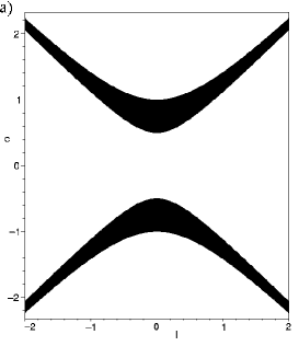
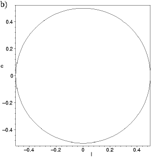
Figure 1: Theoretical boundaries of transverse instability. a) Case (13) with $\sigma=1$. The waves are unstable for the parameters lying within the shaded regions. b) Case (14) with $\sigma=-1$. The waves are unstable for the parameters within the circle.

IV Evans function analysis of the transverse instability

In this section we use the Evans function formalism in order to analyze the linear transverse stability problem for the Boussinesq model (1) for all values of the transverse wavenumber. We restrict attention to the parameter values of most interest: $\varepsilon=-1$ and $D=-1$ associated with the “good” Boussinesq, although we put no restriction on $\sigma$ (but keeping in mind that $\sigma=+1$ is the most interesting case).

However, the class of solitary waves will be enlarged. Namely, we include solitary waves bi-asymptotic to a nontrivial state at infinity, specifically,

$$U(\theta)=U_{\infty}+6\delta^{2}\mathop{\textrm{sech}}\nolimits^{2}\left(\delta\theta\right),\quad\theta=x-ct+ly,$$ (15)

where

$$\delta=\frac{1}{2}\sqrt{\sqrt{1+4a}-c^{2}+\sigma l^{2}}\quad\mbox{and}\quad U_{\infty}=\mbox{$\frac{1}{2}$}(1-c^{2}+\sigma l^{2})-2\delta^{2}=-\frac{2a}{1+\sqrt{1+4a}}\,.$$ (16)

The value of the parameter $a$ is constrained only by existence of the square root: $1+4a\geq(c^{2}-\sigma l^{2})^{2}$.

Here we will not use any geometric structure (although it might be interesting to look more closely in this direction) and so work directly with (1). Let

$$u(x,y,t)=U(\theta)+\Re{\left(\tilde{u}(\theta)\exp\left[iky+\lambda t\right]\right)}.$$ (17)

By substituting this expression in (1) and linearising, one obtains the following equation for the complex function $\tilde{u}(\theta)$

$$\tilde{u}_{\theta\theta\theta\theta}+2(U\tilde{u})_{\theta\theta}-(1-c^{2}+\sigma l^{2})\tilde{u}_{\theta\theta}-2(c\lambda+i\sigma kl)\tilde{u}_{\theta}+(\lambda^{2}+\sigma k^{2})\tilde{u}=0.$$ (18)

After the change of variable $\tilde{x}=\delta\theta$, substitution of the explicit expression for $U$ from (15), and dropping the tildes, equation (18) reduces to

$$u_{xxxx}-4\left[(1-3\mathop{\textrm{sech}}\nolimits^{2}x)u\right]_{xx}-\gamma u_{x}+\beta u=0,$$ (19)

where

$$\gamma=\frac{2(c\lambda+i\sigma kl)}{\delta^{3}}\mbox{ and }\beta=\frac{\lambda^{2}+\sigma k^{2}}{\delta^{4}}.$$ (20)

To obtain explicit solutions of this equation, we note that by taking $u=\phi_{xx}$ and $v=1-3\mathop{\textrm{sech}}\nolimits^{2}x$ in (19), and integrating twice the equation simplifies to

$$\phi_{xxxx}-4v\phi_{xx}-\gamma\phi_{x}+\beta\phi=0.$$ (21)

Solutions of this equation can be readily found in a manner similar to that in B (see also APS ). First we note that in the limit $x\to\pm\infty$, equation (21) reduces to

$$\phi_{xxxx}-4\phi_{xx}-\gamma\phi_{x}+\beta\phi=0.$$ (22)

Substituting now $\phi=e^{\mu x}\hat{\phi}$, one can see that $\mu$ satisfies the quartic equation

$$\mu^{4}-4\mu^{2}-\gamma\mu+\beta=0\,.$$ (23)

Quartics of this form have been analyzed in BD1 (see equation (10.9) there), and when $\Re(\beta)>0$ there are two roots with positive real part and two roots with negative real part. Therefore, the space of solutions decaying as $x\to+\infty$ is two-dimensional, as is the the space of solutions decaying as $x\to-\infty$.

If the four roots $\mu_{j},\mbox{ }j=1,..,4$ of the equation (23) are distinct, the corresponding solutions of (21) are given by

$$\phi_{j}(x)=e^{\mu_{j}x}h_{j}(x),$$ (24)

with

$$h_{j}(x)=(4\mu_{j}^{3}+8\mu_{j}-\gamma)-12\mu_{j}^{2}\mathop{\textrm{tanh}}\nolimits x.$$ (25)

The case of multiple roots can be handled similarly B . Solutions of the original equation (19) are found by substituting $u(x)=\phi(x)_{xx}$, and the other components of the vector ${\bf v}(x)$ can be obtained by the differentiating the expression for $u(x)$.

Localised solutions of the linearised problem exist if one can match the solutions decaying as $x\to\infty$ with the solutions decaying as $x\to-\infty$. This can be determined by finding the zeros of the so-called Evans function which correspond to the eigenvalues of the linearised problem. To define the Evans function, we write the equation (19) as a first-order system

$${\bf v}_{x}=A(x){\bf v},\mbox{ }{\bf v}=\left(\begin{array}[]{l}u\\ u_{x}\\ u_{xx}\\ u_{xxx}\end{array}\right),\mbox{ }A(x)=\left(\begin{array}[]{cccc}0&1&0&0\\ 0&0&1&0\\ 0&0&0&1\\ -\beta+4v_{xx}&\gamma+8v_{x}&4v&0\end{array}\right)$$ (26)

with $v=1-3\mathop{\textrm{sech}}\nolimits^{2}x$.

Since the trace of the matrix $A(x)$ vanishes, the Evans function can be defined as $E(\lambda,k)={\bf v}_{1}(x)\wedge{\bf v}_{2}(x)\wedge{\bf v}_{3}(x)\wedge{\bf v}_{4}(x)$ AGJ . An alternative expression for the Evans function can be derived by using the adjoint system as shown in BD2 . The adjoint system of (26) has the form:

$${\bf w}_{x}=-A(x)^{*}{\bf w},\mbox{ }{\bf w}=\left(\begin{array}[]{l}w_{1}\\ w_{2}\\ w_{3}\\ w_{4}\end{array}\right),$$ (27)

where $A(x)^{*}$ denotes the Hermitian conjugate of $A$ $(A(x)^{*}=\overline{A(x)}^{T})$. The equation for $w_{4}$ turns out to be

$$(w_{4})_{xxxx}-4v(w_{4})_{xx}+\overline{\gamma}(w_{4})_{x}+\overline{\beta}(w_{4})=0.$$ (28)

This equation is equivalent to (21) up to the change of variables: $x\to-x$, $\gamma\to\overline{\gamma}$, $\beta\to\overline{\beta}$, and therefore its solutions can be obtained from (24) by changing $x$ for $-x$ and conjugating them:

$$(w_{4})_{j}=e^{-\mu_{j}^{*}x}\overline{h_{j}(-x)},$$ (29)

with $h_{j}(x)$ defined in (25). Other components of the vector ${\bf w}(x)$ can be obtained from (27).

Let $\mu_{1}$ and $\mu_{2}$ be the two roots of the equation (23) with negative real part, and let ${\bf v}_{j}(x)$ and ${\bf w}_{j}(x)$, $j=1,2$ be the corresponding solution vectors of the linearised (respectively, adjoint) system. Since the matrix $A(x)$ in (26) is traceless, we can define the Evans function for the system (26) as follows BD2 :

$$E(\lambda,k)=\left|\begin{array}[]{cc}\langle{\bf w}_{1}(0),{\bf v}_{1}(0)\rangle&\langle{\bf w}_{1}(0),{\bf v}_{2}(0)\rangle\\ \langle{\bf w}_{2}(0),{\bf v}_{1}(0)\rangle&\langle{\bf w}_{2}(0),{\bf v}_{2}(0)\rangle\end{array}\right|,$$ (30)

where $\langle\cdot,\cdot\rangle$ denotes the complex inner product in $\mathbb{C}^{4}$. To obtain a unique definition of the Evans function, the scaling $\lim_{x\to\infty}e^{-2\mu_{j}x}\langle{\bf w}_{j}(-x),{\bf v}_{j}(x)\rangle=1$ is used. This normalises the eigenvectors and the adjoint eigenvectors of $A^{\infty}=\lim_{x\to\pm\infty}A(x)$.

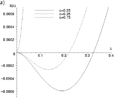
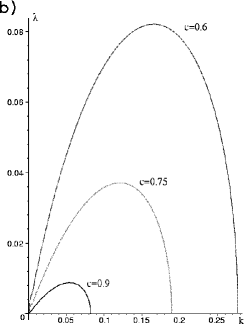
Figure 2: a) The Evans function $E(\lambda)=E(\lambda,0)$ versus $\lambda$ for $c=0.25$, $c=0.35$ and $c=0.75$ respectively. b) Growth rate versus transverse wavenumber for the values of velocity $c=0.6$, $c=0.75$ and $c=0.9$ respectively.

After some lengthy algebra and introducing the scaling, which enforces the asymptotic limit $E(\lambda,k)\to 1$ as $\lambda\to\infty$, the final expression for the Evans function can be obtained, which we do not present here since it is lengthy (the expression for the Evans function as well as the calculations of the instability growth rate can be downloaded as a Maple-file from the website Web ).

Zeros of the Evans function $E(\lambda,k)$ correspond to the bounded solutions of the linearised stability problem with the wavenumber $k$ and the growth rate $\Re(\lambda)$. The leading order terms (in $k$ and $\lambda$) in the Evans function are in complete agreement with the results of the geometric condition of §3. Note that, since the construction here is based on a basic solitary wave with a nontrivial state at infinity, it is suggestive that the geometric condition B1 extends to such waves.

We illustrate the dependence of the Evans function on the wavespeed and transverse wavenumber in Figure 2. In the left graph, the transverse wavenumber is set to zero, to compare with known results on longitudinal instability. The graph is in complete agreement with known results (e.g. BS ; BD1 ) that the solitary wave is stable for $\frac{1}{2}<c\leq 1$ and unstable for $0\leq c<\frac{1}{2}$. In the right-hand graph in Figure 2 we present the plot of the growth rate $\Re(\lambda)$ as a function of the transverse wavenumber. Note that waves of the good Boussinesq which are longitudinally stable are transverse unstable. Note also that there is a cut-off wavenumber, similar to other cases of transverse instability, such as in the Zakharov-Kuznetsov equation AR .

V Post-instability simulations

In this section we perform a simulation of the PDE (1) using the multi-symplectic spectral discretization proposed in BR and applied there to Zakharov-Kuznetsov and shallow-water equations.

The (2+1)-dimensional Boussinesq equation is considered with $\varepsilon=D=-1$ on a finite domain $(x,y)=[0,L]\times[0,L]$ with $L>0$ some constant, and periodic boundary conditions on both spatial variables. We choose a spatial mesh-size as $\Delta x=\Delta y\equiv\Delta m=L/2N$ and introduce the discrete two-dimensional Fourier transform defined as

$$U_{kl}=\frac{1}{\sqrt{2N}}\sum_{i,j=1}^{2N}u_{ij}e^{-\theta_{k}(i-1)\Delta m-\theta_{l}(l-1)\Delta m},$$

where

$$\theta_{k}=i\frac{2\pi(k-1)}{L}$$

and $u_{ij}\approx u(m_{ij}),m_{ij}=(i-1)\Delta x+(j-1)\Delta y$ (cf. F ). Fourier spectral discretization of the (2+1)-dimensional Boussinesq equation yields

$$\partial_{tt}U_{kl}=\bar{\theta}_{k}^{2}\left[\varepsilon\bar{\theta}_{k}^{2}U_{kl}+\nabla_{kl}\bar{F}({\bf U})\right]+\sigma\bar{\theta}_{l}^{2}U_{kl},$$ (31)

where $\bar{\theta}_{k}$ are the entries of the diagonal matrix defined by the relations

$$\bar{\theta}_{k}=\theta_{k},\mbox{ for }k=1,...,N,$$

$\bar{\theta}_{N+1}=0$, and

$$\bar{\theta}_{k}=-\theta_{2N-k+2},\mbox{ for }k=N+2,...,2N$$

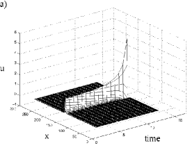
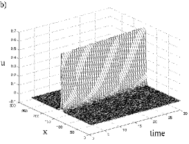
Figure 3: a) Development of the longitudinal instability and collapse at time $t=12$ for $c=\frac{1}{4}$. b) Propagation of a stable solitary wave for $c=\frac{3}{4}$.

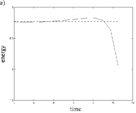
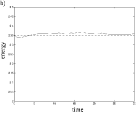
Figure 4: Energy evolution. Dashed line represents the initial energy level, and the solid line shows the time evolution of energy. a) Unstable case $c=\frac{1}{4}$. b) Stable case $c=\frac{3}{4}$.

which follow from the periodicity of the discrete Fourier transform F , and $\bar{F}({\bf U})$ denotes the Fourier transform of the anti-derivative of the function $f(u)$ in (1). The same result would be obtained if one applied the spectral discretization to the multi-symplectic formulation (3), as it was done for the Zakharov-Kuznetsov equation in BR .

For the second-order time derivative we used the central difference approximation (time step was chosen to be $\Delta t=0.01$ in all the simulations):

$$\partial_{tt}U_{kl}=\frac{U_{kl}^{n+1}-2U_{kl}^{n}+U_{kl}^{n-1}}{\Delta t^{2}}.$$ (32)

One should note that the only valid test of this scheme can be done for the “good” Boussinesq equation with $\sigma>0$. For $\sigma<0$ in the case of the “good” Boussinesq equation, an initial profile independent of $x$ would result in a solution which could grow “faster than exponential” because for large transverse wavenumbers, growth rate of the initial data has no upper bound (ill-posedness).

To test the algorithm, we first used it to confirm the results for the dynamics of the one-dimensional solitary waves. The initial profile was taken to be of the form

$$u(x)=\frac{3}{2}\left(1-c^{2}\right)\mathop{\textrm{sech}}\nolimits^{2}\left[\frac{1}{2}\left(1-c^{2}\right)\left(x-\frac{L}{2}\right)\right]+\xi(x),$$ (33)

where $\xi(x)$ is a small random perturbation. The results are presented in Figures 3 and 4. For $c=\frac{1}{4}$ the solitary wave solution is linearly unstable as reported in AS ; BD1 , and the development of this linear instability is shown in Figure 3a). In the case $c=\frac{3}{4}$ the numerical results confirm the stability of the solitary wave (see Figure 3b) ). The simulations were run on an interval of the length $L=256$ with $2N=512$. As a numerical check, the total energy was monitored, and it was found to be well behaved till near the collapse when the significant errors occur, as illustrated in Figure 4.

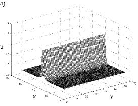
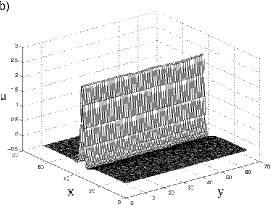
Figure 5: Solitary wave for $\sigma=1$ and $c=\frac{1}{4}$. a) Initial profile. b) Development of the transverse modulation (time $t=11.25$ ).

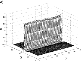
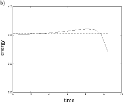
Figure 6: The same as in Fig. 5. a) Wave collapse ( time $t=12$). b) Energy evolution. Dashed line represents the initial energy level, and the solid line shows the time evolution of energy.

For the two-dimensional simulations we took an initial profile in the form of the line solitary wave uniform in $y$

$$u(x,y,0)=\frac{3}{2}\left(1-c^{2}\right)\mathop{\textrm{sech}}\nolimits^{2}\left[\frac{1}{2}\left(1-c^{2}\right)\left(x-\frac{L}{2}\right)\right]+\xi(x,y),$$ (34)

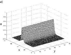
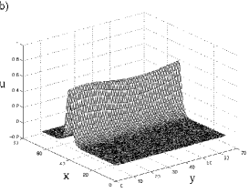
Figure 7: Solitary wave for $\sigma=1$ and $c=\frac{3}{4}$. a) Initial profile. b) Development of the transverse modulation (time $t=184.5$).

where $\xi(x,y)$ is a small random perturbation (in this case $l=0$). The length of the square box was chosen to be $L=64$ with the number of Fourier modes $2N=128$. In the case $c=\frac{1}{4}$ the solitary wave (34) is linearly unstable in longitudinal direction as is known from the stability analysis of the 1D equation. In Figure 5b) we can see this instability developing in a similar way as in the 1D case. One can also note in this Figure the development of the stable transverse modulation. Wave collapse in this case is shown in Figure 6a), with the plot of energy as a function of time in Figure 6b). When $c=\frac{3}{4}$, the solitary wave is longitudinally stable but transversely unstable, and the development of this instability is presented in Figures 7 and 8. We note that at the initial stage of the evolution there is a transverse modulation developing while the amplitude of the wave is gradually growing Figure 7b), then the instability prevails leading finally to the collapse of the wave Figure 8a). Note that this collapse is clearly a two-dimensional effect, since it does not happen uniformly in the $y$-direction. The energy proves to be conserved rather well during the simulations (see Figure 8b) ), although the energy deviates substantially as the wave approaches the stage of collapse.

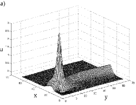
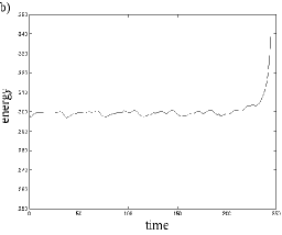
Figure 8: The same as in Fig. 7. a) Wave collapse (time $t=246$). b) Energy evolution. Dashed line represents the initial energy level, and the solid line shows the time evolution of energy.

VI Concluding remarks

We have considered the transverse instability of line solitary wave solutions of the (2+1)-dimensional Boussinesq equation. Using the multi-symplectic formulation of the system, we derived a geometric condition for this instability for small transverse wavenumbers. With an Evans function approach, the linearised stability equation was analyzed, and this allowed to obtain the dependence of the instability growth rate for all transverse wavenumbers. Numerical simulations support the analytical results about transverse and longitudinal instabilities and demonstrate the development of those instabilities and subsequent wave collapse.

We conclude with an open problem. While analytic theories for collapse of solitary waves for the Boussinesq equation in one space dimension exist T , it is an interesting open problem to develop an analytical technique for predicting collapse for the case of two space dimensions, e.g. a generalization of the virial theorem or the result of T for example, and moreover, to determine if transverse instability for (1) leads to collapse for all parameter values.

VII Acknowledgements

The authors would like to thank Sebastian Reich for advice on the numerics and Georg Gottwald for helpful discussions.

References

- (1) J.C. Alexander, R. Gardner, C.K.R.T. Jones, J. Reine Angew. Math. 410, 167 (1990).
- (2) J.C. Alexander, R.L. Pego, R.L. Sachs, Phys. Lett. A 226, 187 (1997).
- (3) J.C. Alexander, R.L. Sachs, Nonlinear World 2, 471 (1995).
- (4) M.A. Allen, G. Rowlands, J. Plasma Phys. 50, 413 (1993).
- (5) M.A. Allen, G. Rowlands, Phys. Lett. A 235, 145 (1997).
- (6) J.G. Berryman, Phys. Fluids 19, 771 (1976).
- (7) K.B. Blyuss, http://www.maths.surrey.ac.uk/personal/pg/K.Blyuss/
- (8) B.N. Breizman, V.M. Malkin, Sov. Phys. JETP 52, 435 (1980).
- (9) J.L. Bona, R.L. Sachs, Comm. Math. Phys. 118, 15 (1988).
- (10) T.J. Bridges, Phys. Rev. Lett. 84, 2614 (2000).
- (11) T.J. Bridges, J. Fluid Mech. 439, 255 (2001).
- (12) T.J. Bridges, G. Derks, Phys. Lett. A 251, 363 (1999).
- (13) T.J. Bridges, G. Derks, Arch. Rat. Mech. Anal. 156, 1 (2001).
- (14) T.J. Bridges, G. Derks, University of Surrey Preprint, 2001 (to be published).
- (15) T.J. Bridges, S. Reich, Physica D 152-153, 491 (2001).
- (16) B. Fornberg, A practical guide to pseudospectral methods (Cambridge University Press, Cambridge, 1996).
- (17) E. Infeld, G. Rowlands, A. Senatorski, Proc. Roy. Soc. Lond. A 455, 4363 (1999).
- (18) R.S. Johnson, J. Fluid Mech. 323, 65 (1996).
- (19) B.B. Kadomtsev, V.I. Petviashvili, Sov. Phys. Dokl. 15, 539 (1970).
- (20) Y.S. Kivshar, D.E. Pelinovsky, Phys. Rep. 331, 117 (2000).
- (21) E.A. Kuznetsov, A.M. Rubenchik, V.E. Zakharov, Phys. Rep. 142, 104 (1986).
- (22) E.W. Laedke, K.H. Spatschek, Phys. Rev. Lett. 41, 1798 (1978).
- (23) S.K. Turitsyn, Phys. Rev. E 47, R796 (1993).
- (24) X.P. Wang, M.J. Ablowitz, H. Segur, Physica D 78, 241 (1994).
- (25) V.E. Zakharov, Sov. Phys. JETP 26, 994 (1968) 994.