Short time decay of the Loschmidt echo

Abstract

The Loschmidt echo measures the sensitivity to perturbations of quantum evolutions. We study its short time decay in classically chaotic systems. Using perturbation theory and throwing out all correlation imposed by the initial state and the perturbation, we show that the characteristic time of this regime is well described by the inverse of the width of the local density of states. This result is illustrated and discussed in a numerical study in a 2-dimensional chaotic billiard system perturbed by various contour deformations and using different types of initial conditions. Moreover, the influence to the short time decay of sub-Planck structures developed by time evolution is also investigated.

I INTRODUCTION

Quantum irreversibility studies have become a very active research topic due to a direct connection with quantum computers and mesoscopics physics qcomputer ; mesos . The natural quantity for these investigations has been introduced by Peres in his seminal paper of 1984 peres . Called later as Loschmidt echo (LE) or fidelity, it measures the ability of a system to return to an initial state $|\phi\rangle$ after a forward evolution with a Hamiltonian $H_{0}$ followed by an imperfect reversal evolution with a perturbed Hamiltonian $H=H_{0}+\delta xH^{\prime}$ ($\delta x$ parameterize the strength of the perturbation). Thus, it is given by

$$M(t)=|\left\langle\phi\right|\exp[{\rm i}Ht]\exp[-{\rm i}H_{0}t]\left|\phi\right\rangle|^{2}$$ (1)

(throughout the paper $\hbar$ is set equal to 1). The LE compares the evolution of an initial state with slightly different Hamiltonians and can distinguish regular and chaotic classical dynamics peres ; jalabert ; jaquod1 .

The LE was recently studied in various chaotic systems using several approaches jalabert ; jaquod2 ; tomsovic ; fernando1 ; prosen ; wisniacki1 ; fernando2 ; wisniacki2 . However, few types of decay were discussed in the literature. For a very short time, it is straightforward to show that the LE has a parabolic behavior $M(t)=1-\delta x^{2}(\Delta H^{\prime})^{2}t^{2}$, with $(\Delta H^{\prime})^{2}=[\langle\phi|H^{\prime 2}|\phi\rangle-\langle\phi|H^{\prime}|\phi\rangle^{2}]$. This decay is better resembled by the Gaussian function $\exp[-(t/\tau)^{2}]$, with characteristic time $\tau=1/(\Delta H^{\prime}\delta x)$. Though this regime has experimental relevance LEexp , it has not been extensively taken into account.

After this short time decay, a crossover to a perturbation dependent regime was predicted and numerically observed jalabert ; tomsovic ; jaquod2 ; fernando1 ; wisniacki1 . For very small $\delta x$, in which a typical matrix element $U$ of the perturbation is smaller than the mean level spacing $\Delta$, the decay is always Gaussian until $M(t)$ reaches its asymptotic values $M(t\rightarrow\infty)\equiv M_{\infty}$. If $U>\Delta$, this regime has an exponential decay $\exp(-\Gamma t)$, with $\Gamma$ the width of the local density of states (LDOS). This is usually called Fermi golden rule regime (FGR). When $\Gamma>\lambda$, with $\lambda$ the mean Lyapunov exponent of the classical system, a perturbation independent regime is observed. In this case, the decay rate is given by $\lambda$. Finally, if $\Gamma$ exceeds the bandwidth of the perturbation, the LE has a Gaussian decay.

The properties of the initial state play an important role in the behavior of the LE jaquod2 ; wisniacki2 . This point can be relevant to observe the mentioned regimes. For example, the Lyapunov regime is not displayed if the initial state is an eigenfunction of the unperturbed/perturbed Hamiltonian wisniacki2 . Localized wave packets are needed to observe this regime. On the other hand, Zurek has recently stated that dynamical evolution causes that these states develop a sub-Planck structures in phase space, and he predicts that these structures enhance their sensitivity to perturbations zurek .

In this article we are mainly interested in the short time decay of the LE. Disregarding system specific features and the correlations imposed by the characteristics of initial state, we show via perturbation theory that $\tau^{-1}$ is given by the width $\Gamma$ of the LDOS. In order to see the validity of this result in a realistic model, we study the characteristic time $\tau$ in a paradigmatic model of quantum chaos, a 2-D chaotic billiard perturbed by a contour deformation. We regard the influences of the characteristics of the perturbation and the initial condition to this important regime. Therefore, we consider different perturbations and various types of initial conditions in our numerical study. We find that some perturbations, which we call generic, destroy correlations imposed by the initial condition giving that $\tau^{-1}=\Gamma$. Nevetheless, other perturbations do not act in that way and this fact produces a slower decay with $\tau^{-1}<\Gamma$. In this context, we discuss the influence of an initial time evolution of the wave packet and the corresponding developed structures in phase space in the short time decay of the LE. In fact, it is shown that an initial dynamical evolution helps to erase the mentioned correlations, with the effect of increasing $\tau^{-1}$. If the initial evolved time is smaller than the Ehrenfest time, the enhanced decay is described entirely by the classical streaching arround the unstable manifold given by the Lyapunov exponent jaquodsubplanck . But for greater evolved times, the quantum interference lead a developed sub-planck structure in phase space and this yield that the decay continuos growing. That is, the sensitivity to perturbations is also enhanced in this case (as stated in Ref. zurek ). However , if the perturbation produces a decay with $\tau^{-1}=\Gamma$ the developed structures in phase space do not influence the short time decay.

The paper has the following structure. Sec. II is devoted to describe the model system and the various shape deformations that we have considered. The paper is self-contained with the inclusion of the shape parameter Hamiltonian expansion for a 2-D quantum billiards developed in Ref. wisniacki3 . In Sec. III, the characteristic time $\tau$ is related to the width of the LDOS using perturbation theory. Then, in Sec. IV we present the numerical results. We study the LE for several types of initial condition. Starting with the simplest case when the initial state is an eigenfunction of $H_{0}$, we follow with Gaussian wave packets. Finally the initial conditions are the evolved Gaussian wave packets in order to study the prediction of Ref. zurek . In Sec. V we make some final remarks.

II MODEL SYSTEM: DEFORMED STADIUM BILLIARDS

We use the desymmetrized Bunimovich stadium billiard as a model system to explore the behavior of the LE wisniacki1 . This paradigmatic system is fully chaotic and has great theoretical and experimental relevance cit-bunimovich ; cit-marcus-dephas-dot ; cit-marcus-def-dot . It consists of a free particle inside a 2-dimensional planar region whose boundary ${\cal C}$ is shown in Fig.  1 with dashed lines. The radius $r$ is taken equal to unity and the enclosed area is $1+\pi/4$.

The system is perturbed by boundary deformations which preserves the area of the billiard. Deformations with different characteristics are chosen in order to understand their influences in the short time decay of the LE. Fig.  1 shows the shape deformations that have been considered. The changes of the boundary are parameterized by

$${\bf r}(s,\delta x)={\bf r_{0}}(s)+z(s,\delta x)\;{\bf n}\;,$$ (2)

with $s$ along ${\cal C}$, ${\bf r_{0}}(s)$ the parametric equation for ${\cal C}$, and ${\bf n}$ the outward normal unit vector to ${\cal C}$ at ${\bf r}_{0}(s)$ (see Fig.  1(a)). Case (a), shown in Fig.  1, is well described in Ref. wisniacki3 . For deformation (b)-(d), $z(s,\delta x)=\alpha\delta x\cos(\pi Ns/P)$ with $\alpha=0.42$, $P=1+\pi/2$ and N=3, 5 and 10. $\alpha$ is chosen in order that the width of the LDOS of all deformations are aproximately equal in the studied range of $\delta x$ . As we shall see in the next section, the width of the LDOS is a measure of the magnitude of a perturbation.

Figure 1: Schematic figure of the system and the various shape deformations. Desymmetrised stadium billiard is plotted with dashed lines. On continuous lines, deformations of the billiard are shown. The curvilinear coordinates used to describe the deformations [Eq. 2] is also included.

To solve Eq. (1), eigenvalues and eigenfunctions of perturbed and unperturbed system are needed. They are obtained using a Hamiltonian expansion of deformed billiards which has been recently developed wisniacki3 . For $\delta x\leq 1/k_{0}$ ($k_{0}$ the mean wave number of the region under study), the eigenenergies and eigenfunctions of the deformed billiard, are connected to the ones of the stadium by the linearized Hamiltonian expressed in the basis of eigenstates at $\delta x=0$ (from now on we will call $\phi_{\mu}$ to these eigenstates and $E_{\mu}$ the respective eigenenergies) ,

$$H_{\mu\nu}(\delta x)\simeq H_{\mu\nu}(0)+\delta x\;H^{\prime}_{\mu\nu},$$ (3)

with $H_{\mu\nu}(0)=E_{\mu}\delta_{\mu\nu}$ and

$$H^{\prime}_{\mu\nu}=-{\rm Cf}_{\mu\nu}\;A_{\mu\nu}\oint_{{\zeta}}z^{\prime}(s)\;\frac{\partial\phi_{\mu}}{\partial{\bf n}}\frac{\partial\phi_{\nu}}{\partial{\bf n}}ds.$$

The eigenfunctions and eigenenergies at $\delta x=0$ are obtained using the scaling method cit-Vergini-Saraceno . The integral above could be viewed as an inner product among the wave functions $\frac{\partial\phi_{\mu}}{\partial{\bf n}}$ defined over ${\cal C}$. This relation defines an effective Hilbert space in a window $\Delta k\approx$ Perimeter/Area wisniacki3 . The cut-off function ${\rm Cf}_{\mu\nu}=\exp\left[-2\;(k_{\mu}^{2}-k_{\nu}^{2})^{2}/(k_{0}\Delta k)^{2}\right]$ restricts the effect of the perturbation to states in this energy shell of width $k_{0}\Delta k$. It allows to deal with a basis of finite dimension with wave numbers around the mean value $k_{0}$, restricting to a particular region $\Delta k$ of interest. We are considering $k_{0}=100$ and $2m=1$ ($m$ the mass of the particle) in all the numerical calculations presented above.

III SHORT TIME DECAY AND THE LOCAL DENSITY OF STATES

Our aim is to characterize the short time decay of the LE. As mentioned in the introduction, a simple calculation led the short time decay to depend on the initial state and on the perturbation peres . We want to relate the characteristic time $\tau$ of the short time decay with some general properties of the perturbation.

The influence of a perturbation over a quantum system could be described by the local density of states (LDOS). The LDOS of an unperturbed eigenstate $\phi_{\mu}$ is defined as

$$\rho_{\mu}(E,\delta x)=\sum_{\nu}{|\langle\phi_{\nu}(\delta x)|{\phi_{\mu}}\rangle|^{2}\delta[E-(E_{\nu}(\delta x)-E_{\mu})]},$$ (4)

with $E_{\nu}(\delta x)$ and $\phi_{\nu}(\delta x)$ the energy and eigenfunction of the perturbed Hamiltonian [Eq. (3)]. This function shows how the unperturbed states are coupled to the perturbed ones. Because we are not interested in a particular state, an implicit average over the unperturbed state $\mu$ is considered from now on. We have chosen the width (dispersion)

$$\Gamma(\delta x)=\sqrt{\sum_{\nu}{\rho_{\mu}(E_{\nu}(\delta x)-E_{\mu},\delta x)(E_{\nu}(\delta x)-E_{\mu})^{2}}},$$ (5)

as a practical measure of this distribution .

The LDOS exhibits various regimes as a function of the strength $\delta x$ dcohenannal ; dcohenpara . As we shall see, the perturbative regime is relevant for our study. Perturbation theory (PT) gives the following first order expression for the LDOS

$$\rho_{\rm PT}(E,\delta x)=\delta(E)+\frac{|H^{\prime}_{\mu\nu}|^{2}\delta x^{2}}{[E_{\nu}(\delta x)-E_{\mu})]^{2}}\delta[E-(E_{\nu}(\delta x)-E_{\mu})].$$ (6)

Using the definition of the width [Eq. (5)] and Eq. (6) it is straightforward to show

$$\Gamma_{\rm PT}(\delta x)=\delta x\sqrt{\sum_{\nu}|H^{\prime}_{\mu\nu}|^{2}}.$$

This expression works very well for all the perturbations of Fig 1 with strength $\delta x\leq 1/k_{0}$.

With these ingredients in mind, let us consider the short time decay of the LE. As pointed out previously, it is given by $M(t)=\exp[-(t/\tau)^{2}]$ with $\tau^{-2}=(\langle\phi|H^{\prime 2}|\phi\rangle-\langle\phi|H^{\prime}|\phi\rangle^{2})\delta x^{2}$. Let be $|\phi\rangle=\sum{a_{\mu}\phi_{\mu}}$ the initial state , so

$$\tau^{-2}=[\sum{a_{\mu}H^{\prime}_{\mu i}H^{\prime}_{i\nu}a_{\nu}}-(\sum{a_{\mu}H^{\prime}_{\mu\nu}a_{\nu}})^{2}]\delta x^{2}$$ (7)

The perturbation matrix $H^{\prime}_{\nu\mu}$ is a banded matrix due to the cut-off function ${\rm Cf}_{\mu\nu}$ (see the insets of Fig. 2). This band structure is quite generic in realistic systems due to the finite range interaction of unperturbed states band1 ; band2 . Inside the band, the matrix elements $H^{\prime}_{\mu\nu}$ are highly fluctuating numbers. At first sight if we ignore the system specific features, we can do the diagonal approximation of Eq. 7, resulting

$$\tau^{-2}=[\sum{|a_{\mu}|^{2}H^{\prime 2}_{\mu\nu}}]\delta x^{2}.$$ (8)

This approximation is also valid for the case in which the complex numbers $a_{\mu}$ behave randomly. Finally, if we consider that the $|a_{\mu}|^{2}$ are nearly constant inside the band,

$$\tau^{-2}\approx[\sum{H^{\prime 2}_{\mu\nu}}]\delta x^{2}=\Gamma^{2}_{\rm PT}(\delta x).$$ (9)

This result is also valid if $a_{\mu}=\delta_{\mu\nu}$, assuming that we are averaging over several initial conditions. Note that we have obtained Eq. (9) throwing out all the correlations imposed by the perturbation and the wave amplitudes. In the next section we will see in what manner these correlations influence the decay.

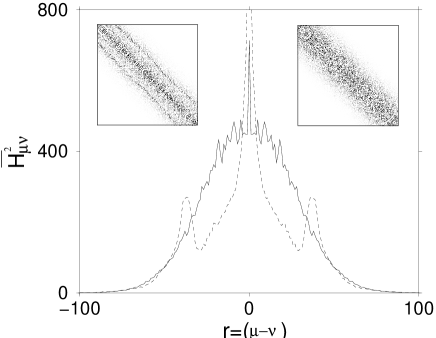
Figure 2: Mean value of the matrix elements $H^{\prime 2}_{\mu\nu}$ as a function of $r=\mu-\nu$ for the deformations (a) (dotted line) and (d) (full line). The peak for the deformation (a) is due to the bouncing ball orbits. Insets: Image of a piece of the perturbation matrix $|H^{\prime}_{\mu\nu}|$ shown as a density plot. The left plot corresponds to the perturbation label as (a) and the right plot corresponds to perturbation label as (d). Clearly, there is a structure in the perturbation matrix for pertubation (a) when compared to perturbation (d).

Each perturbation is characterized by the structure and correlations of the matrix elements $H^{\prime}_{\mu\nu}$. As an example, Fig. 2 shows the behavior of the mean value of $H^{\prime 2}_{\mu\nu}$ as a function of the distance $r=\nu-\mu$ for perturbations (a) and (d). This function is usually called band profile. The cases (b) and (c) are not plotted because their band profile are qualitative equal to case (d). Note that perturbation (a) is clearly non-generic due to the two important peaks at $|r|\sim 25$. This non-universality is introduced by the fact that perturbation (a) does not connect the bouncing ball states with generic states. In the insets of Fig.  2 a density plot of these matrix are shown for deformations (a) and (d). We will see in the next section that there are correlations between the matrix elements of the perturbation which are not exposed in the band profile but have an important influence to the short time decay.

IV NUMERICAL RESULTS

In this section we study numerically the behavior of the short time decay of the LE in the Bunimovich stadium billiard perturbed by the contour deformation presented in Sec. 1. We consider different types of initial conditions: Eigenfuction of $H_{0}$, Gaussian wave packets and evolved Gaussian wave packets . We would like to see the range of validity of Eq. 9 for our particular system.

IV.1 Eigenfuctions of $H_{0}$

The simplest case of the LE is when the initial state of Eq. 1 is an eigenstate of ${\cal H}_{0}$. In this case, the LE is directly related with the Fourier transform (FT) of the LDOS. Then, $M(t)$ is the so called survival probability wisniacki2 ; Cohen-Heller , defined as

$$P(t)=|\left\langle\phi_{\mu}\right|\exp[{\rm i}Ht]\left|\phi_{\mu}\right\rangle|^{2}=|FT[\rho_{\mu}(E,\delta x)]|^{2}$$ (10)

As we saw in the previous section, we expect that $\tau$ for $\bar{P}(t)$ is well described by Eq. 9. $\bar{P}(t)$ is the mean value of the survival probability over several initial states. We have numerically observed that this is the case for the perturbations (b-d). These results are shown in Fig. 3. Note that $\tau^{-1}$ for perturbations (c) and (d) are not plotted because the results are the same as (b). The widths $\Gamma(\delta x)$ and $\Gamma_{PT}(\delta x)$ are equal for all the perturbations. For perturbation (a), $\tau^{-1}\approx 0.85\Gamma(\delta x)$ which is directly related to the structure of the perturbation matrix (see Fig. 2) imposed by the bouncing ball states wisniacki1 . Similar attenuation was observed in Ref. wisniacki1 for perturbation (a) in the FGR regime. In this case, the decay rate is given by $0.5\Gamma(\delta x)$ insted of the expected value $\Gamma(\delta x)$.

Figure 3: $\tau^{-1}$ of the survival probability as a function of $\delta x$ when the system is perturbed by deformations (a) and (b). The width of the LDOS $\Gamma(\delta x)$ and its perturbative evaluation $\Gamma_{PT}(\delta x)$ calculated using Eq. (6) are also plotted.

Figure 4: $\bar{P}(t)$ for the desymmetrized stadium billiard perturbed by deformation (d) of Fig. 1. The values of the strength of the perturbation is $\delta x=0.015$ for the top curve and 0.05 for the bottom curve. The dashed lines correspond to the Gaussian decay $\exp[-(\Gamma(\delta x)t)^{2}]$ and the exponential decay $\exp[-(\Gamma(\delta x)t)]$ is plotted with a dotted line.

Fig. 4 summarizes the behavior of $\bar{P}(t)$ in the desymmetrized stadium billiard. We have taken an average over 100 initial states. In this figure, the results for perturbation (d) of Fig. 1 are shown. Other perturbations led to the same qualitative results. For a small perturbation strength (top curve of Fig. 4) we observe the Gaussian short time decay and after that an exponential decay with a decay rate given by the width of the LDOS jaquod1 ; wisniacki1 . For large perturbation strength (bottom curve of Fig. 4) the exponential decay with decay rate given by $\Gamma(\delta x)$ is not observed . This is due to the constraint imposed by the asymptotic value $M_{\infty}$. In this case the decay is completely Gaussian. An important point is that the asymtotic $M_{\infty}\approx\Delta/\Gamma(\delta x)$.

IV.2 Localized Gaussian wave packets

The decay of the LE for localized Gaussian wave packets has been widely studied in the literature. Most of the previous works consider this case jalabert ; jaquod2 ; wisniacki1 ; fernando1 ; fernando2 . The predicted crossover from a perturbation dependent regime to the Lyapunov regime has been shown for these classically adapted initial conditions.

We discuss here the short time decay of the LE for this particular type initial conditions in the stadium billiard perturbed by deformations presented in Fig. 1. We compute $M(t)$ for initial Gaussian wave packets,

$$\phi(\vec{r})=(\pi\sigma^{2})^{1/2}\exp{[i\vec{p}_{0}.(\vec{r}-\vec{r}_{0})-i|\vec{r}-\vec{r}_{0}|^{2}/\sigma^{2}]}$$ (11)

with $|p_{0}|=k_{0}=100$ and $\sigma=0.16$. An average over 50 initial states was taken. The direction of the momentum $\vec{p}_{0}/|\vec{p}_{0}|$ and the center of the wave packet $\vec{r}_{0}$ are chosen randomly. As expected, the short-time decay is well described by a Gaussian function $\exp[-(t/\tau)^{2}]$. Fig. 5 shows the behavior of $\tau^{-1}$ as a function of the strength $\delta x$ for all the perturbations under study. This type of initial conditions imposes correlations so that the second sum of right hand side of Eq. (7) does not vanish. The non-universalities of each perturbation are clearly exposed in $\tau$. Note that these differences are not seen in the width of the LDOS nor in band profile of the matrix $H^{\prime}_{\mu\nu}$. We have considered perturbations with greater number of oscillations of the boundary ($N>10$) and we find $\tau=1/\Gamma(\delta x)$ for all of them wisniacki4 .

Figure 5: $\tau^{-1}$ of $\bar{M}(t)$ as a function of $\delta x$ when the system is perturbed by deformations (a), (b), (c) and (d). The initial states are the Gaussian wave packets of Eq. (11). $\Gamma(\delta x)$ is also plotted in solid line.

IV.3 Evolved Gaussian wave packets

In a recent paper zurek , Zurek shows that dynamical evolution of initial Gaussian wave packets in classically chaotic systems, produces finer and finer phase space structures which saturates after the Ehrenfest time with a sub-Planck scale. More important, he predict that this sub-Planck structures enhances the sensitivity of a quantum state to an external perturbation. A numerical study in a time dependent one dimensional model agreed with this assertion karkuszewski , but other studies reached opposite conclusions jaquodsubplanck ; jordan . In Ref. jaquodsubplanck it is showed an enhanced decay of the LE of evolved wave packets but this acceleration is fully described by the classical Lyapunov exponent and it is not due to the sub-Planck structures. More specifically, it is pointed out that the characteristic time $\tau(T_{0})$ of the short time decay for a wave packet that has been evolved a time $T_{0}$ is given by

$$\tau^{-1}(T_{0})=\tau^{-1}(0)\exp(\frac{\lambda(T_{0}-T_{c})}{2}),$$ (12)

with $\tau(0)$ the characteristic time of the short time decay for initial states that have not been evolved, $\lambda$ the Lyapunov exponent and $T_{c}$ the mean time for the first collision with the boundary.

We consider the influence of the developed structures in phase space in the short time decay of the LE. So, $M(t)$ is computed for the same initial conditions [Eq. (11)] of the previous section but an unperturbed initial evolution during a time $T_{0}$ is applied. Fig. 6 shows $\tau^{-1}(T_{0})$ as a function of the strength $\delta x$ for perturbation (a) and with $T_{0}=0,0.025,0.05,$ and 1. Note that $\tau^{-1}(T_{0})$ increases with larger $T_{0}$, for all perturbation strenghts. This fact clearly points out that an initial evolution enhances the sensitivity to this particular perturbation. We have observed that for $T_{0}>0.4$, $\tau^{-1}$ converges to the width of the LDOS. Same behavior is shown when the system is perturbed by deformations (b) and (c). However, when the perturbation destroys the correlations imposed by the initial wave packet which implies that $\tau=1/\Gamma$, the short time decay is not affected by an initial evolution.

Figure 6: $\tau^{-1}$ of $\bar{M}(t)$ as a function of $\delta x$ for perturbations (a). The initial states are Gaussian wave packets that have been evolved a time $T_{0}$. $\Gamma(\delta x)$ is also plotted.

In order to see if these increments are fully described by Eq. 12 and due to that has classical nature, in Fig.7 it is showed the behavior of $\tau^{-1}(T_{0})/\tau^{-1}(0)$ for several preparation time $T_{0}$ for perturbation (a) with strenght $\delta x=0.04$. It is clearly observed that Eq. 12 works well for $T_{0}<0.025$. Note that the Ehrenfest time $T_{E}=0.025$. So, the enhacement of the short time decay is fully explained with the classical inestability given by the Lyapunov exponent for evolved times $T_{0}$ smaller than the Ehrenfest time. However, for larger times $\tau^{-1}(T_{0})$ is also growing.

A qualitative picture of acceleration of the short time decay for evolved states is the following. Before the Ehrenfest time the wave packet is streaching around an unstable manifold and just after that times starts the quantum interference which lead a sub-Planck structures. At that times a small part of the Wigner function presents a sub-Planck structure. This region grows with time and it seems to be the reason of the accelerating decay. Note that for the saturation times the sub-Planck structure is all arround the available phase space.

Figure 7: $\tau^{-1}(T_{0})/\tau^{-1}(0)$ as a function of the preparation time $T_{0}$ for strenght $\delta x=0.04$. The stadium is perturbed by deformation (a). The prediction of Ref. jaquodsubplanck (Eq. 12) is ploted in solid line.

V FINAL REMARKS

We have studied the short time decay of the LE in a 2-D chaotic billiard. The system was perturbed by a contour deformation. Different perturbations were considered in order to develop the influences of their characteristics in the behavior of the LE. Moreover, several types of initial conditions have been used and how they affect the LE have been examined.

Our findings are the following. For non-localized initial states and if the system is perturbed by a generic deformation, the characteristic time $\tau$ of the short time Gaussian decay is given by the inverse of the width $\Gamma$ of the LDOS. If semiclassical features are exposed in the matrix elements of the perturbation, we have obtained that $\tau^{-1}<\Gamma$. For highly localized initial states, cross correlation between wave amplitudes are important and this is exposed with the fact that $\tau^{-1}<\Gamma$. When the perturbation destroys such correlations, the characteristic time $\tau^{-1}$ exhibits its maximum value $\Gamma$.

We have discussed the prediction of Zurek zurek which stated that an initial dynamical evolution of semiclassical wave packets lead a sub-Planck structures in phase space and this enhances its sensitivity to perturbation. We found that in the cases in which the perturbation does not destroy the correlation mentioned before an accelerated decay is observed. As a function of the preparation time $T_{0}$, we have observed two regimes. For $T_{0}$ smaller than the Ehrenfest time, the enhanced decay is described entirely by the classical Lyapunov exponent as pointed out in Ref. jaquodsubplanck . However, for larger $T_{0}$ in which the quantum interference lead the sub-Planck structures the enhancement of decay is also observed.

A final point is worth commenting. We have shown that the short time decay of the LE has a Gaussian behavior and for certain perturbations the characteristic time is given by the width of the LDOS. The LDOS of some systems Cohen-Heller ; dcohenpara ; wisniacki2 ; note presents a region in which its width is independent of the perturbation. We note that these results could be of importance for the understanding of the measure of the LE in recent NMR experiments LEexp . Although that system consists of many interacting nuclear spins, the results are in accordance with the former. That is, due to imperfections in the reversed evolution the LE in the MNR experiment shown a Gaussian attenuation, $M(t)=\exp[(t/\tau)^{2}]$, with $\tau$ depending on the small non-inverted interaction (which corresponds to the perturbation $\delta xH^{\prime}$ of Eq. 1), and in a range of small perturbation, the characteristic time $\tau$ do not depend on it.

References

- (1) M. A. Nielsen and I. L. Chuang, Quantum Computation and Quantum Information (Cambridge University Press, Cambridge, 2000).
- (2) Y. Imry, Introduction to mesoscopic Physics (Oxford, New York, 1997)
- (3) A. Peres, Phys. Rev. A 30, 1610 (1984).
- (4) R.A. Jalabert and H.M. Pastawski, Phys. Rev. Lett. 86, 2490 (2001).
- (5) Ph. Jacquod, I. Adagideli and C.W.J. Beenakker, nlin.CD/0206160.
- (6) Ph. Jacquod, P.G. Silvestrov and C.W.J. Beenakker, Phys. Rev. E 64, 055203 (2001).
- (7) N.R. Cerruti and S. Tomsovic, Phys. Rev. Lett. 88, 054103 (2002).
- (8) F.M. Cucchietti, H. M. Pastawski and D. A. Wisniacki, Phys. Rev. E 65 045206(R) (2002).
- (9) T. Prosen and M. Znidaric, J. Phys. A 35 ,1455 (2002).
- (10) D.A. Wisniacki, E. G. Vergini, H. M. Pastawski and F. M. Cucchietti, Phys. Rev. E 65 055206 (R) (2002).
- (11) F.M. Cucchietti, C. H. Lewenkopf, E. R. Mucciolo, H. M. Pastawski and R. O. Vallejos, Phys. Rev. E 65 046209 (2002).
- (12) D.A. Wisniacki and D. Cohen, Phys. Rev. E 66, 046209 (2002)
- (13) H. M. Pastawski, P. R. Levstein, G. Usaj, J. Raya and J. Hirschinger, Physica A, 283 166 (2000).
- (14) W. H. Zurek, Nature 412, 712 (2001).
- (15) Ph. Jacquod, I. Adaglideli and C.W.J. Beenakker, Phys. Rev. Lett. 89, 154103 (2002).
- (16) D. A. Wisniacki and E. Vergini, Phys. Rev. E 59, 6579 (1999).
- (17) L. A. Bunimovich, Funct. Anal. Appl. 8 254 (1974).
- (18) A. G Huibers et al. Phys. Rev. Lett, 83 5090 (1999)
- (19) M. Switkes, C. M. Marcus, K. Campman and A. C. Gossard, Science 283, 1905 (1999).
- (20) E. Vergini and M. Saraceno, Phys. Rev. E 52, 2204 (1995).
- (21) D. Cohen, Phys.Ann. Phys. (N.Y.) 283, 175 (2000).
- (22) A. A. Gribakina, V. V. Flambaum, and G. F. Gribakin, Phys. Rev. E 52, 5667 (1995).
- (23) W. Wang, F. M. Izrailev, and G. Casati, Phys. Rev. E 57 323 (1998).
- (24) D. Cohen, A. Barnett and E.J. Heller, Phys. Rev. E 63, 46207 (2001).
- (25) D. Cohen and E. Heller, Phys. Rev. Lett. 84 2841 (2000).
- (26) D.A. Wisniacki, unpublished.
- (27) Z. P. Karkuszewski, C. Jarzynski and W. H. Zurek, Phys. Rev. Lett. 89, 170405 (2002).
- (28) A. Jordan and M. Srednicki, quant-ph/0112139.
- (29) Our system do not exhibit such a region due to inclusion of the cut-off function. This region can be observed for large enough but in this case we can not deal with the numerics.