Nonlinear dynamics of waves and modulated waves in 1D thermocapillary flows.
II: Convective/absolute transitions.

Abstract

We present experimental results on hydrothermal waves in long and narrow 1D channels. In a bounded channel, we describe the primary and secondary instabilities leading to waves and modulated waves in terms of convective/absolute transitions. Because of on the combined effect of finite group velocity and of the presence of boundaries, the wave-patterns are non-uniform in space. We also investigate non-uniform wave-patterns observed in an annular channel in the presence of sources and sinks of hydrothermal waves. We connect our observations with the complex Ginzburg-Landau model equation in the very same way as in the first part of the paper [1].

and

Introduction

Non-linear traveling-waves have exhibited a fascinating variety of behaviors and patterns. Waves systems have been studied in binary-fluid convection (subcritical traveling waves bifurcation) [2, 3], oscillatory instability in low Prandtl number convection [4], oscillatory rotating convection [5] and cylinder wake [6]. One of the main source of richness in wave patterns is the existence of two different regimes: the convective and the absolute one [7, 8]. This distinction arises when the group velocity of the waves in non-zero. The convective/absolute transition between those two regimes leads to critical phenomena of important relevance in wave-systems. We present here the first complete description of convective/absolute transitions for traveling waves in finite a box for both primary and secondary instability onset.

Most 1D physical systems produce right- and left-propagating non-linear waves [9]. Non-linear competition and reflections at the boundaries then lead to a central-source pattern [10, 11, 12, 13] due to counter-propagating exponentially growing waves as the first global mode at onset. But the global mode may also be produced at the convective/absolute transition as we will illustrate. So far, this phenomenon was described for single waves [7, 14, 15], i.e., with broken left-right symmetry.

Hydrothermal waves [16, 17, 18, 19] provide very interesting and generic systems of traveling waves which can be modelized by envelope equations such as the complex Ginzburg-Landau equation (CGL) [20, 21]. The present paper is the second part of an article devoted to the connection between hydrothermal waves and those amplitude equations. We will further refer to the companion paper [1] as I.

In I, we present the experimental hydrothermal waves systems, and the periodic solutions obtained in an annular cell. We will often refer to this paper, but we recall here in Section 1 the main characteristics of our systems and some important results. The present paper is mainly devoted to the case of a rectangular cell, i.e., of a long narrow channel with non-periodical boundary conditions. We show that hydrothermal waves realize as in I an ideal supercritical non-linear wave system in accordance with theoretical predictions in such a bounded geometry: convective and absolute transitions have to be taken into account to describe the effect of the group velocity over the onsets of both primary and secondary instabilities. We also present results in an annular cell with periodic boundary conditions in the special case where the periodicity is broken by the pattern itself.

In Section 2, we study first the critical behavior at the primary onset for a finite cell with low-reflection boundaries. When the wave pattern appear, it is qualitatively very different from the uniform hydrothermal waves (UHW) pattern observed within periodic boundary conditions and described in I, through the governing equations are the same. This results from the broken Galilean invariance due to the existence of boundaries. We will show that the first global mode, instead of being constructed by successive reflections in the convective regime, results from the onset of absolute instability. The onset of this mode —corresponding to the convective/absolute transition— is shifted above the value corresponding to convective instability. This is illustrated in Fig. LABEL:fig:A_vs_DT of I and we will detail qualitatively and quantitatively how the transition occurs. Some experimental critical exponents are discussed in the framework of existing theoretical descriptions and a quantitative comparison with complex Ginzburg-Landau model is proposed.

Section 3 is devoted to modulated waves. For higher values of the control parameter, the wave pattern undergoes a secondary modulational instability; we present the convective/absolute transition for this instability in the bounded channel. This instability is of the same nature as the Eckhaus instability occurring on UHW in the annular channel and described in the companion paper I: it leads also to a wave-number selection in the rectangular channel. We will introduce fronts of spatio-temporal defects and link them to the convective and absolute nature of the instability.

In section 4, we show that the convective/absolute transitions have reminiscent effects in the annular geometry, when sources and sinks exist that break the Galilean invariance as physical boundaries do. The group velocity term cannot be cancelled out of the equations anymore where such objects are present. This leads to qualitative and quantitative behaviors predicted theoretically [9] and observed in our experimental system; we then confirm the pertinence of the convective/absolute instability transitions.

1 The rectangular geometry and the wave model

The experimental system has been described in section LABEL:sec:setup and Fig. LABEL:fig:schema_rect of the companion paper I [1]. We study the traveling-waves instability of a thermocapillary flow obtained when applying an horizontal temperature gradient over a thin liquid layer with a free surface. Let us emphasize that we use annular and rectangular channels of both the same width $10$mm, and that the fluid height is $h=1.7$mm for all experiments reported in the present paper. The curvature is negligible [22], and we have shown by stability analysis [23] that its effects on critical values are of order $3.10^{-2}$, so both wave pattern reports can be directly connected. Please note that the channel length will be noted $L_{\rm b}$ for the bounded (rectangular) channel and $L_{\rm p}$ for the periodic (annular) channel. Without subscript, $L$ will concern the current channel, and $L^{*}$ the non-dimensional length $L/\xi_{0}$ where $\xi_{0}=5.1$mm is the coherence length of the pattern (see section LABEL:sec:model in I). We have $L_{\rm b}=180$mm and $L_{\rm p}=503$mm; the aspect ratios in both cells ensure that patterns are one-dimensional.

The control parameter is the horizontal temperature difference $\Delta T$ between the two long sides of the container. The fluid is observed using shadowgraphy and taking care of being in the linear regime (see I), i.e., we record the shadowgraphic image on a screen located at a distance much larger than the focal distance of the convection pattern, even for larger values of the temperature constraint [22]. The first bifurcation of the basic thermocapillary flow towards hydrothermal waves occurs in the annulus for $h=1.7$mm at $\Delta T_{\rm c}=(3.1\pm 0.1)$K as described in section LABEL:sec:hydrothermal of I. The bifurcated pattern for hydrothermal waves is then a uniform-amplitude traveling wave of critical wavenumber $k_{0}=(0.684\pm 0.003)$mm^-1 and critical frequency $f_{0}=0.237$Hz. In the rectangular geometry, boundaries act as sources or sinks and in fact both right and left traveling waves are present at threshold. So hydrothermal waves must be modeled by two slowly varying amplitudes $A$ and $B$ obeying two complex Ginzburg-Landau equations:

$$\tau_{0}(A_{T}+sA_{X})=\epsilon(1+ic_{0})A + \xi_{0}^{2}(1+ic_{1})A_{XX}$$

$$- g(1+ic_{2})|A|^{2}A-g(\lambda+i\mu)|B|^{2}A$$

$$\tau_{0}(B_{T}-sB_{X})=\epsilon(1+ic_{0})B + \xi_{0}^{2}(1+ic_{1})B_{XX}$$ (1)

$$- g(1+ic_{2})|B|^{2}B-g(\lambda+i\mu)|A|^{2}B$$

$\epsilon=(\Delta T-\Delta T_{\rm c})/\Delta T_{\rm c}$ is the reduced distance from threshold. Boundary conditions for $A$ and $B$ should be included with this description. Perturbations are verified to travel at the group velocity $v_{g}$ in the rectangular box as well as in the annular one. Please note that in the CGL Eqs (1), $s$ denotes the value of the group velocity $v_{g}$ at the convective onset. The coefficients $\tau_{0}$, $c_{0}$, $c_{1}$, $c_{2}$, $g$, $\lambda$ and $\mu$ are all real and commented in I.

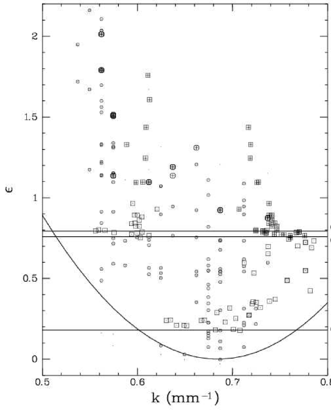
Figure 1: Experimental stability diagram for hydrothermal waves at $h=1.7$mm. Data are presented for both annular ($\circ$) and rectangular ($\Box$) geometry. In the annulus, small circles stand for homogeneous waves. Modulated waves are depicted with and additional cross $+$. In the rectangle, no waves are observed below $\epsilon_{\rm a}=0.18$, and for $\epsilon>\epsilon_{\rm m,c}=0.76$ points are grouped on two different vertical branches. Those branches correspond to two different wave trains at the same time within the cell. An additional $+$ in the squares denotes that those waves are modulated. $\epsilon_{\rm m,c}$ and $\epsilon_{\rm m,a}$ stands for the onset of convective and absolute modulational instability (Section 3). The solid parabola is the measured marginal stability curve.

In order to quantitatively connect results in annular and rectangular geometry, we propose in Fig. 1 a representation of stable states in the annulus together with all states obtained in the rectangle. In this figure, as in all the text in this article, $\epsilon$ is defined for both experiments using the onset in the annulus. Wavenumbers are expressed in such a way that they do not depend on the size of the system, so we use dimensional unit (mm^-1). In the annulus, we observe uniform hydrothermal waves (UHW), i.e., waves with constant amplitude, wavenumber and frequency and modulated waves (MW), i.e., waves with modulated amplitude, wavenumber and frequency. The existence of UHW and MW suggest that the wave system may be described using phase equations. Please note that in the annulus, no particular selection of the wavenumber exists within the stability zone of UHW, except the restriction of that the wavenumber must be an integer when expressed in $(2\pi/L)$ units. In the rectangle, no such restriction exists and the wavenumber can take any value.

Let’s describe the states observed in the rectangular channel. First, we note that between $\epsilon=0$ and $\epsilon=\epsilon_{\rm a}=0.18$, we never observe waves. This fact will be detailed in Section 2 presenting the primary onset. When increasing the control parameter from the threshold value $\epsilon_{\rm a}$, the wavenumber $k$ increases while exploring the whole band of allowed wavenumbers.

Above $\epsilon\simeq 0.45$, a smooth selection process occurs and the wavenumber $k$ is of order of $21\cdot(2\pi/L_{\rm b})\simeq 0.73$mm^-1: this correspond to the vertical branch on the right of the stability diagram. For $\epsilon>\epsilon_{\rm m,c}\sim 0.758\pm 0.01$, the waves are modulated and two regions are observed in the cell, corresponding to two different mean wavenumbers. The first region corresponds to the previous right branch and the other to the left branch of the diagram, with $k\sim 17\cdot(2\pi/L_{\rm b})\simeq 0.59$mm^-1. This selection process is rather sharp. Above $\epsilon_{\rm m,a}$, any state in the cell is represented by a point on each of the two branches. Between $\epsilon_{\rm m,c}$ and $\epsilon_{\rm m,a}$, the left branch is only populated by transients. The splitting of the $(k,\epsilon)$ curve in two branches is due to the Eckhaus instability and will be carefully detailled in section 3.

Please note that far from onset, wavenumbers are either greater or smaller than the critical one and in fact the two branches observed are away from $k=k_{\rm c}=(0.684\pm 0.003)$mm^-1 (Section 2.6 of I).

Let’s also note that in the rectangle, due to the non-periodic boundary conditions, the amplitude is forced to vanish or have very low values, thus jeopardizing any phase description. Our wave-system is such that the boundaries at $x=0,L$ are poorly reflective [17]: we have indications that the reflection coefficient is within the range $10^{-3}-10^{-1}$.

Please note that for sufficiently high $\epsilon$ ($\geq 1$), we observe the same asymmetrical selection of wavenumbers $k<k_{\rm c}$, as the annulus. This global selection confirm the relevance of higher order terms perturbing the amplitude equation (Section LABEL:sec:model in I). However, let’s emphasize that when considering the primary onset, i.e., small value of $\epsilon$ and small amplitudes $A$ and $B$ of the waves, we may neglect the higher order terms. In contrast, when presenting the Eckhaus instability leading to the selection of lower wavenumbers, one should include those higher order terms to perform a correct analysis of the secondary instability.

The main result from Fig. 1 is the perfect overlap of the zones of existence. Stable waves —Stokes solutions of the CGL eqs (1)— are observed in the rectangle and in the annulus in the same region of the $(k,\epsilon)$ plane. Moreover, modulated waves, and so the Eckhaus instability, occur in the same regions. Though the spatial extents of the cells are different, they are both extended and the global wavenumber selection process looks the same: as $\epsilon$ is increased, the wavenumber is expected to be lower. The overlap also confirm that coefficients in amplitude equations are likely to be identical in both geometries (Section LABEL:sec:model in I).

2 Onset of primary wave instability in the rectangle

We describe here how the wave pattern appears and evolves near the primary onset. As explained, for small values of $\epsilon$ as those considered here, higher order terms can be neglected in the amplitude equations and we believe that usual Complex Ginzburg-Landau equations for traveling waves are sufficient for the description of the primary onset. In the following we choose, for clarity, to present the major wave as $A$ (right-traveling) and the minor wave as $B$ (left-traveling), but the reverse situation has been observed with equal probability.

2.1 Description of the patterns

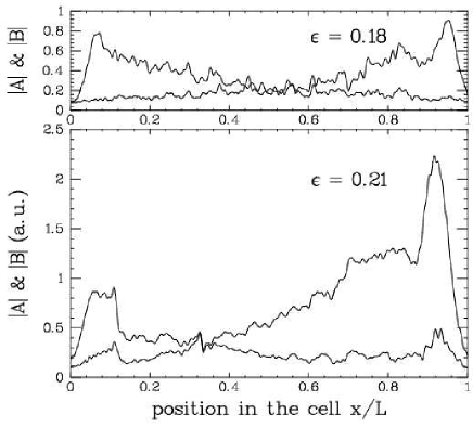
Figure 2: Amplitude profiles of the traveling waves at different $\epsilon$. Top figure presents right ($A$) and left ($B$) amplitude profiles for $\epsilon=0.18$ ($\Delta T=3.66$K) and bottom figure for $\epsilon=0.21$ ($\Delta T=3.75$K).

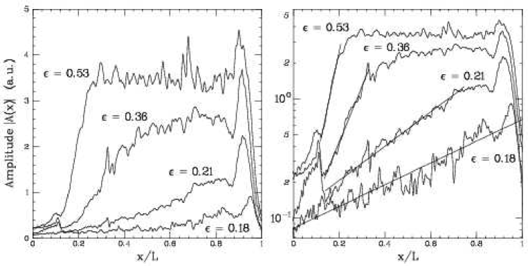
Figure 3: Amplitude profiles of the dominant traveling wave for growing $\epsilon$ up to $0.53$ ($\Delta T=4.75$K). On both figures, the data is the same; left: linear scale; right: logarithmic scale. All dominant waves are represented as right-traveling waves. Following the wave, we encounter three domains: an exponential growth or front, a saturated plateau (for larger $\epsilon$), and a sharp wall-mode. The linear fits on the lin-log plot give the value of the exponential spatial growth rate $\xi_{\rm F}^{-1}$. Similarly, spatial growth $\xi_{\rm WM}^{-1}$ and decay rate $\xi_{\rm down}^{-1}$ can be fitted on both sides of the wall-mode on the right side of the plot.

Figure 4: Amplitude ratio $B/A$ for both averaged amplitude $\langle A\rangle$ over the cell ($\circ$) and maximum amplitude $A_{\rm max}$ ($+$). See text for details. Solid line is an exponential fit. As $\epsilon$ is increased higher above onset, the minor wave disappear.

Typical amplitude profiles in the rectangle for $A$ and $B$ are shown on Figs. 2 and 3 for various temperature differences. For $\Delta T<\Delta T_{\rm a}=3.65$K ($\epsilon<\epsilon_{\rm a}=0.177$), no wave is observed and so $A=B=0$. Just above onset, for $\Delta T=3.66$K, we observe a symmetric wave-pattern (Fig. 2). As $\Delta T$ is increased above $\Delta T_{\rm a}$, i.e., $\epsilon$ is increased above $\epsilon_{\rm a}$, one wave becomes dominant and invade a larger region of the cell (Fig. 3). The waves compete up to $\epsilon\simeq 0.25$, above which the smallest wave becomes negligible with respect to the dominant wave (Fig. 4). The wave envelope of the dominant wave may be seen as composed of three domains: (i) just after the wall $X=0$ which may also be called source, where both amplitude $A$ and $B$ are nearly zero, there is a front where the amplitude is exponentially growing; this is illustrated on Fig. 3. (ii) after the front, a plateau is present for higher values of $\Delta T$; (iii) finally, just before the end wall $X=L$, the amplitude profile has a bump and maximum amplitude is reached here, in what is called a wall mode.

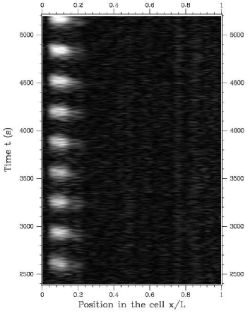
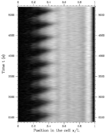
Figure 5: Blinking state: spatio-temporal diagram of the local amplitude showing the perodical oscillations of the source separating the right- and left-traveling waves for $\epsilon=0.36$ ($\Delta T=4.21$K). Left : left-traveling wave. Right : right-traveling wave. The wave amplitude is proportional to the gray level of the images but for the minor (left) wave, amplitude has been multiplied by a factor of 2. Black corresponds to zero amplitude. A low-frequency beating is observed with a period around 320s.

In the front region, we can compute for each realization the spatial growth rate of the amplitude envelope $|A(X)|$ from the source, as shown in Fig. 3. The front can be described by an exponential envelope ${\rm e}^{\xi_{\rm F}^{-1}X}$ where $\xi_{\rm F}^{-1}$ is the growth rate. The characteristic length $\xi_{\rm F}$ is linked to the front critical behavior [17] and will be described in the next paragraph. Please note that the spatial growth rate in the source region is well defined both close to the onset, and far from the onset.

The plateau is vanishing in the vicinity of the threshold and so it cannot be used to quantify the critical behavior. Quantitative description of the bifurcation are given in terms of the wall-mode amplitude and the front spatial growth rate.

Please note that the amplitude is almost vanishing at the boundaries $X=0$ and $X=L$. This is an indication for a very low reflection coefficient in our system [24].

When $\epsilon\gtrsim 0.3$, the states are not always stationary and we observe quasi-periodic realizations corresponding to a beating of minor and major waves. Those states were called “blinking states” [10, 25, 12, 13]. Such a realization is presented in Fig. 5. We believe that the occurrence of such quasi-periodic patterns is due either to reflections at the boundaries between both counter-propagating waves and/or to the nonlinear competition between counter-propagating waves. This scheme is detailed in Section 2.3.

Figure 6: Spatial profile of the local wavenumber $k$ in the rectangle together with the amplitude profile, for $\Delta T=3.75$K. Though noisy, the wavenumber is well defined far from the source region. $k$ is fairly constant except in the wall mode region where amplitude variations are large.

2.2 Quantitative results

Fig. 6 presents a typical wavenumber measurement. We obtain its value everywhere the amplitude is large enough to allow measurements: we discard regions in which the amplitude is less than 0.5 (a.u.). We then note than except in the wall-mode region where amplitude variations are large, the local wavenumber is almost constant in the cell. The mean wavenumber is computed by averaging values far from the boundaries. It is close to $k\sim 21\cdot(2\pi/L_{\rm b})\simeq 0.73$mm^-1. Measured values of frequency and wavenumber are presented on Fig. 7. We note that they match the annulus critical values at onset, as seen in the stability diagram (Fig. 1). For higher values of the control parameter, frequency and wavenumber are multivalued; this results from the existence of a new branch of solutions as presented on Fig. 1. This new branch appears when the primary wavenumber becomes unstable with respect to modulational instability (Section 3).

Computing the velocity at which perturbations are advected allows us to compute the group velocity. The corresponding data is represented in Fig. 8, togheter with the phase velocity of the waves. Here again, for clarity, we distinguish between waves of different wavenumbers, i.e., we distinguish between the two branches in the stability diagram. Of importance is the fact that the group velocity is always finite and large. Note that the value of $v_{g}$ at $\epsilon_{\rm a}$ is the same as the one at onset in the annulus, i.e., $v_{g}(\epsilon_{\rm a})=s$. The phase velocity is about twice the group velocity.

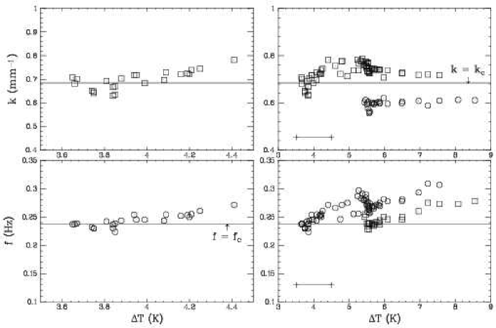
Figure 7: Frequency and wavenumber in the rectangle vs. $\Delta T$. Full horizontal lines show the critical values from annular cell data. On the left are shown zooms on the region [3.5K, 4.5K] corresponding to the primary instability and represented on the right figures by a segment. Different symbols are used for the two branches of solutions for higher values of $\Delta T$; those branches correspond to mean wavenumber $21\cdot(2\pi/L_{b})=0.73$mm^-1 and $17\cdot(2\pi/L_{b})=0.59$mm^-1. See also Fig. 1.

Figure 8: Phase velocity $v_{\phi}$ and group velocity $v_{g}$ in the rectangle vs. $\Delta T$. $\Box$ stands for waves of mean wavenumber close to $21\cdot(2\pi/L)$ (the right branch in Fig. 1) and $\circ$ for waves of mean wavenumber close to $17\cdot(2\pi/L)$ (the left branch in Fig. 1). The group velocity is always finite and lower than the phase velocity. The symbol at $\epsilon=0$ stands for $s$, the group velocity at onset in periodical geometry and the dashed line recalls the linear fit obtained in periodical geometry (Fig. LABEL:fig:vg_annulus in I).

Let’s now present the critical behavior of the front using the spatial growth rate $\xi_{\rm F}^{-1}$ defined in the previous paragraph. On Fig. 9 are presented such data and possible fits. Following the simplest intuition, we can propose a linear fit for the data; this leads to an estimation for the threshold at 3.65K. A closer observation of the experimental points at 3.66K suggests this may not be the best description very close to onset: we have conducted several experiment, at $\epsilon=\epsilon_{\rm a}$, and all led to a small but finite value of $\xi$, larger than the error bar. We also tried a square-root law, pertinent close to the onset but jeopardized for values of $\epsilon$ a bit larger. Following the authors of Refs [26, 15], we then searched for a linear relation between $\xi$ and $\ln(\epsilon-\epsilon_{\rm a})$ and found a better agreement for all experimental points within a broader range, and most of all close to the threshold. The physical meaning of this logarithmic critical behavior will be discussed below.

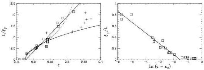
Figure 9: Critical behavior of the spatial growth rate characterizing the front region. Left graph shows experimental data ($\Box$ for stationary states and $+$ for blinking states) togheter with a linear fit, a square root fit (solid lines) and a logarithmic fit (dashed line). Fits are performed on stationary data ($\Box$) only. The graph on the right present the logarithmic fit $\xi_{\rm F}\propto\ln(\epsilon-\epsilon_{\rm a})$. See text for details.

Let’s look at the amplitude in Fig. 3 and search to define another order parameter of the transition. The amplitude being non uniform, two quantities are easily extracted: the averaged and the maximum value of the amplitude profile, both represented in Fig. 10. The average amplitude $\langle|A(X)|\rangle_{[0,L]}$ evolves linearly with respect to $\epsilon$ (Fig. 10b), but shows a small finite step at $\epsilon_{\rm a}$. On the other hand, the maximum $A_{\rm{max}}$ which occurs near the downstream boundary, at the top of the wall-mode, behaves like $(\epsilon-\epsilon_{\rm a})^{1/2}$ (Fig. 10a). We believe it to be the order parameter of this supercritical bifurcation. Please note that this quantity is studied here very carefully around its onset $\epsilon_{\rm a}$, while a global view is given in I over a wide range of $\epsilon$ in order to compare to the annular geometry which bifurcate at $\epsilon=0$. Finally, as noted in the previous paragraph, the saturation amplitude within the plateau region cannot be measured close to the transition. This does not allow one to conclude anything about the threshold value; a linear fit of the squared amplitude versus $\epsilon$ even leads to an incorrect value of the onset (Fig. 10c).

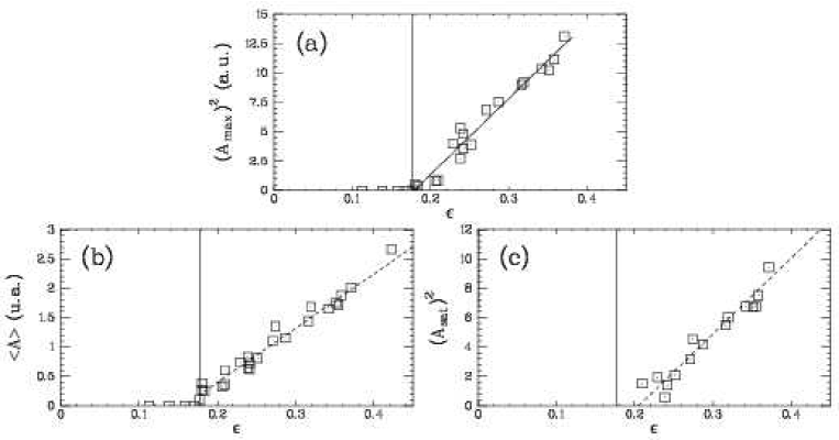
Figure 10: Critical behaviors in the rectangle for (a): the maximum amplitude $A_{\rm max}$, i.e., the modulus of the wall-mode, (b): the mean amplitude $\langle|A(X)|\rangle_{[0,L]}$, and (c): the amplitude of the plateau. The vertical line represent the onset value $\epsilon_{\rm a}=0.18$ ($\Delta T=3.65$K). Only the amplitude of the wall-mode has a critical behavior in accordance with the observed onset value.

Last, the ratio of the two amplitudes $A$ and $B$, plotted on Fig. 4, behaves like $\exp(-\alpha\frac{\epsilon-\epsilon_{\rm a}}{\epsilon_{\rm a}})$ with $\alpha=3.0$. This is observed both for the averaged amplitudes $(\langle|A|\rangle,\langle|B|\rangle)$ and the maximum (wall-mode) amplitude $(A_{\rm max},B_{\rm max})$. The decrease of the minor wave is effective as soon as $\epsilon>\epsilon_{\rm a}$; this is different from the behavior observed in [10]. It denotes a strong competition between the two waves. Due to the power law increase of the maximum amplitude, this reveals the exponential disappearance of the minor wave when $\Delta T$ is increased.

2.3 Discussion

2.3.1 Onset shift

The onset shift between the annular cell and rectangular cell experiments is well interpreted using the convective/absolute transition. This shift along with the critical behavior of the front have been described in [17, 27]. On the hydrodynamic point of view, a linear stability analysis of the thermocapillary problem in a finite box [28] has revealed a particular spatial growth rate —an envelope of the main unstable mode— at onset, together with a shift of this onset from the value computed in infinite geometry.

The shift of the onset is very large: $0.18$ in $\epsilon$ or $0.55$K in $\Delta T$. Usual finite size effect are known to be of order $(\pi/L^{*})^{2}$, i.e., $0.01$ in $\epsilon$ for the $L^{*}=35$ rectangular channel. This law has been verified with a good accuracy for hydrothermal waves in a variable rectangular cell [29]. Another difference between the two cells is the curvature. This can be quantified by a linear stability analysis of the thermocapillary problem [22, 23]: in the annulus, the curvature increases the onset by $0.03$ in $\epsilon$. None of these effects explains the $0.18$ shift.

So what in the rectangle makes the first global mode, or self-excited wave, observed above $\epsilon_{\rm a}=0.18$ ? Below $\epsilon_{\rm a}$, no waves are observed and we unsuccessfully tried to trigger wave-trains with mechanical perturbations (but not with thermal perturbations which should be more efficient as tested within a hot wire experiment [30]).

2.3.2 Global eigenmode of the CGL model

In the periodic channel, once the convective onset is crossed, a traveling wave (TW) self-organizes after successive rounds in the cell: the basic uniform TW is a global mode and both convective and absolute onset collapse [7]. This corresponds mathematically to the Galilean invariance of the problem in the annulus : one can eliminate the group velocity $s$ by studying the problem in a frame moving at velocity $s$. In the non-periodic channel however, $s$ is finite and the problem has to be solved in the laboratory frame. The first global mode is then observed when the growth rate is large enough not to have the waves envelope advected away by the group velocity. This correspond to the transition between convective and absolute instabilities of the primary wave-pattern. This transition occurs in the complex Ginzburg-Landau equation when $\epsilon$ reaches the critical value $\epsilon_{\rm abs}$ given by:

$$\epsilon_{\rm abs}=\frac{1}{1+c_{1}^{2}}\left(\frac{s\tau_{0}}{2\xi_{0}}\right)^{2}$$ (2)

Below $\epsilon_{\rm abs}$, waves are convectively unstable in infinite geometries [31, 32] and no global mode exists in finite non-periodical geometry [14]. For $\epsilon=\epsilon_{\rm a}$, the global mode in a bounded system of size $L$ is of the form:

$$A(x)=A_{\rm gm}\sin\left(\pi\frac{X}{L}\right)e^{(1-ic_{1})\xi_{\rm abs}^{-1}X}\qquad~{}\xi_{\rm abs}=(1+c_{1}^{2})\frac{2\xi_{0}^{2}}{s\tau_{0}}$$

In the vicinity of this threshold, the global mode amplitude is predicted to behave as $A_{\rm gm}\propto(\epsilon-\epsilon_{\rm a})^{1/2}$.

We proposed [17] that our system exhibit the transition from convective to absolute instability at the onset of the waves in the rectangular cell. This conjecture can be summarized as:

$$\epsilon_{\rm a}=\epsilon_{\rm abs}.$$ (3)

The spatial structure of the predicted global eigenmode is an exponential growth with a spatial growth rate $\xi_{\rm abs}^{-1}$ independent of $\epsilon$. The main feature of the observed pattern, however, is the fast varying $\xi_{\rm F}$ of the front region (Fig. 9). Very close to $\epsilon_{\rm a}$, we observe that the wall-mode is well visible (Fig. 3) This wall-mode shows a spatial growth, measured between the plateau and the maximum, which is independent of $\epsilon$ (Fig. 11a). This measure is difficult to perform because the wall-mode growth is almost hidden by the front mode, but it appears clearly that the wall mode is a good candidate for the global eigenmode. Quantitative measurements [17] confirms this hypothesis allowing to measure the value of characteristic time coefficient $\tau_{0}$.

After the maximum of the wall-mode, one can finally measure a spatial damping rate $\xi_{\rm down}^{-1}=(39\pm 4)L^{-1}=(1.36\pm 0.14)$mm^-1 for the envelope of the wave in the wave sink in the vicinity of $X=L$ (Fig. 11b). Within the error bars, this quantity is independent of $\epsilon$, and is comparable to the wavelength of the hydrothermal wave. This results is similar to the observation of the damping in the core of wave sinks by Pastur et al.[33]. One may suspect non-adiabatic effects to be responsible for this property. CGL may not be the right model to describe the sink cores.

Note also that for higher values of $\epsilon$, the theory [14] predicts a wavenumber selection by the front, exactly as we observe: $k\simeq 21(2\pi/L)\simeq 0.73$mm^-1 instead of $k_{c}=0.68$mm^-1.

Figure 11: (a): spatial growth rate $\xi_{\rm WM}$ of the wall-mode measured upstream to the wall-mode as the spatial growth rate of the bump. (b): spatial damping rate $\xi_{\rm down}$ of the envelope of the wave measured downstream of the bump, close to $X=L$. $\xi_{\rm WM}$ and $\xi_{\rm down}$ are almost constant with respect to the control parameters.

2.3.3 Effect of wave reflections

This scenario is not the only way to explain a shift in the threshold. Cross et al. [34, 12, 13] proposed a different mechanism involving the two opposite traveling waves and their mutual reflections at the boundaries $x=0$ and $x=L$. It is found that waves can be observed only for $\epsilon>\epsilon_{\rm r}$ where:

$$\epsilon_{\rm r}=-s\tau_{0}L^{-1}\ln(r)+{\rm O}(L^{-2})$$ (4)

where $0\leq r\leq 1$ is a real number, interpreted as a reflection coefficient of one wave into the opposite one at the boundary. Martel and Vega [35, 36] explored this theory much further, explaining how a global mode is constructed for two waves in a bounded geometry. Their analysis also used the reflection coefficient $r$ between the two waves at the boundaries and the nonlinear coupling between the two waves. They recovered the experimental succession of states described by Croquette and Williams [10], i.e., the existence of a full range in $\epsilon$ where the two-waves pattern is symmetrical. Furthermore, they described the secondary instability; but they discarded the effect of the group velocity, i.e., the convective/absolute transition, through it is of great importance in finite boxes [14].

The conjecture (3) is equivalent to $\epsilon_{\rm abs}<\epsilon_{\rm r}$ for the hydrothermal waves system. Owing to poor reflections in the rectangular cell with Plexiglas ends, we believe that this is pertinent and that $\epsilon_{\rm r}$ is large.

Finally, another experimental fact confirms our conjecture. The experimental sequence of competition between right- and left-wave with $\epsilon$ (Fig. 2, 3 and 5) is the following: symmetric state $\rightarrow$ asymmetric state $\rightarrow$ quasi-periodic blinking state $\rightarrow$ “filling” state, i.e., a single wave. This sequence fits the description in case of reflection-controlled mechanism [12, 13, 35, 36] except that the initial symmetrical pattern exists only for $\epsilon=\epsilon_{\rm a}$ instead of existing over a finite range as is the case in the reflection-controlled mechanism, and observed experimentally in that case [10, 13].

Blinking states are observed in our experiment for $\epsilon\gtrsim 0.3$, we may suggest that this value could be an upper estimate for $\epsilon_{\rm r}$. It can also be interpreted as the fact that nonlinear interactions become important for such higher values of the control parameter.

At the present time, a complete model taking into account both the convective/absolute transition and the role of the reflection coefficient and the nonlinear coupling remains to be done in the case of a two-waves system.

2.3.4 The nature of the convective/absolute transition

The last question we wish to address concerns the nature of the convective/absolute. We observed that the front size behaves logarithmically around $\epsilon_{\rm a}$ (Fig. 9). This behavior has been detected experimentally by Gondret et al. [15] in nonlinear surfave waves and is the signature, in the sense of Chomaz and Couairon [26], of a nonlinear convective/absolute transition. A linear transition [14, 26] would show the front size to behave as $(\epsilon-\epsilon_{\rm a})^{-1/2}$. This has a practical consequence on the experimental observation: since all derivatives of the spatial growth rate are infinite at $\epsilon_{\rm a}$, the front appears much faster with $\epsilon$ than the eigenmode. This explains why the eigenmode is almost hidden by the front and may be detected only as a faint wall-mode in the close vicinity of $\epsilon_{\rm a}$.

For a better observation of the eigenmode one can suggest to increase the length $L$ of the channel. The results of Pastur et al. [33] for a long hot-wire experiment could have lead to such observation. However, since $\epsilon_{\rm r}$ decreases with $L$ (Eq. 4), these authors report another result: below $\epsilon_{\rm a}$ (refered to by $\epsilon_{\rm so}$), they observe fluctuating sources due to the amplification of experimental noise by the convective instability. Near $\epsilon_{\rm a}$, a crossover leads to non-fluctuating sources, comparable to the front we observe: the sources are located in the middle of the channel and not at one end, but their size also critically depend of $\epsilon$. However, since waves and sources are already present in the convective region below $\epsilon_{\rm a}$, the transition itself is also hidden and its nature cannot be detected.

By increasing the length of our cell and/or by reducing the length of Pastur et al. cell [33] we are confident that one could make the connection between the two experimental observations: to observe the eigenmode as clearly as we do below a certain critical channel length, and then analyse how the convective wave becomes visible below $\epsilon_{\rm a}$ when $L$ gets long enough for $\epsilon_{\rm r}$ to become smaller than $\epsilon_{\rm a}$.

3 Onset of secondary modulational instability in the rectangle

Experiments on non-linear traveling waves have been frequently carried in annular cells [4, 2, 6, 5, 16] for the simplicity of the underlying wave pattern. In such periodic geometries, despite an eventual shift on the onset [37, 38], the Eckhaus instability is always absolute. Nevertheless, this instability, as the primary one, may be convective when the group velocity cannot be canceled out of the equations [39, 40]. Moreover, the main specificity of our wave-system is to become Eckhaus unstable for increasing values of the control parameter, i.e., as a first step on the route to spatio-temporal chaos [1, 16].

As shown in Fig. 1, this secondary instability is non-symetrical in $k-k_{c}$; we proposed in Section LABEL:sec:model of I that higher order terms should be included in the amplitude equation. Such terms are of importance when considering secondary instability because $\epsilon$ is then no longer small.

Evaporation is limiting the duration of experiments and refills strongly perturb the patterns. So, in order to get long data series close to onsets, we generally used a protocol in which refills are made just before acquisition starts and long thermal stabilization time are avoided: the temperature gradient is first established in the vessel, the cell is refilled and the fluid is agitated to break the thermal gradients. Within a few seconds the hydrothermal waves reappear without history, i.e., without any special values of the wavenumber, or any special position of dislocations within the cell. However, such a protocol makes it difficult to test the presence of hysteresis at the transitions with control parameter $\epsilon$.

3.1 Wave system

From the previous section we know that for $\epsilon>0.45$ ($\Delta T>4.5$K), a single wave is present in the cell with constant amplitude, wavenumber and frequency (Fig. 3). This pattern constitutes now our basic state and the present section focus on the secondary instability of this single wave train for higher values of $\epsilon$. We choose it to be a right-traveling wave and write its amplitude as $A$.

In the absence of modulations, this wave train is uniform. This is illustrated in Fig. 12a: the local and instantaneous wavenumber is homogeneous in the cell and constant in time. When modulations are present, as in Fig. 12b, we perform a second demodulation to compute the amplitude of this modulation, as well as its wavenumber and frequency. This second Hilbert transform is computed over a spatio-temporal image of the carrier phase derivative (wavenumber or frequency).

As the group velocity is finite, all perturbations, including the modulational ones, are advected. We will show the relevance of a new object, namely a front: a dislocations front or a modulations front. In periodic conditions (section LABEL:sec:annulus of I), this modulational instability occurs at the lowest possible wavenumber $K_{\rm mod}=2\pi/L_{\rm p}$ [16, 37]: it is strictly an Eckhaus [41] instability. In the rectangular channel, we will also refer to Eckhaus instability, although the wavenumber of the modulational instability modes are somewhat bigger: typically $K_{\rm mod}\sim 4\!\cdot\!(2\pi/L_{\rm b})$; it is a finite wavenumber instability.

In the following, we describe the observed regimes starting from the absolute one obtained for higher values of the control parameter; we then present the convective and seemingly stable regimes for smaller values of $\epsilon$.

3.2 Absolute instability and corresponding states

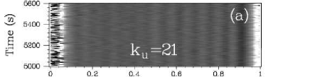
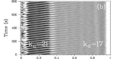
Figure 12: Spatio-temporal diagrams of the local and instantaneous wavenumber $k(x,t)$ of the wave: temporally stabilized regimes for (a) $\epsilon=0.79$, $\Delta T=5.54$K and (b) $\epsilon=0.82$, $\Delta T=5.65$K. The waves propagate from left to right. The mean wavenumber can be estimated visually by the mean gray level and is labeled (units $2\pi/L$) in the upstream ($k_{\rm u}\simeq 21\cdot(2\pi/L)$) and downstream ($k_{\rm d}\simeq 17\cdot(2\pi/L)$) regions. A uniform wavenumber (a) corresponds to an homogeneous state and illustrates both stable and convective regimes below $\Delta T_{\rm m,a}$. It is the asymptotic regime obtained after the transient shown in Fig. 13, left. The modulated state (b) is the global mode of the Eckhaus instability. Each black to white transition of the wavenumber value at $x_{F}/L=0.32$ is due to a phase jump in the core of a defect. The defect front is stable along time. (c) By Hilbert demodulation of phase-gradient image (b) we get the spatial profile of the amplitude $A_{\rm mod}$ of the modulation, presented here in logarithmic units.

Figs 12 and 13 presents the three states which support our discussion. For $\epsilon>\epsilon_{\rm m,a}=0.79$ or $\Delta T>\Delta T_{\rm m,a}=(5.56\pm 0.03)$K, the observed pattern (Fig. 12b) can be described as a wave composed of two wave-trains of mean wavenumbers $k_{\rm u}$ and $k_{\rm d}$. The wavenumber, frequency and amplitude of both wave-trains are modulated in space and time. The wavenumber $K_{\rm mod}$ of the modulation is of order of $|k_{\rm u}-k_{\rm d}|$. Waves are emitted by one side of the cell with wavenumber $k_{\rm u}\sim 21\!\cdot\!(2\pi/L)\simeq 0.73$ mm^-1 and propagate along the cell at the phase velocity. The phase modulation of this wave-train, traveling at the group velocity, is spatially growing. in Fig. 12c, we clearly see the exponential growth of the local-wavenumber modulation amplitude $A_{\rm mod}$ along $x$. At a fixed, finite distance $x_{F}$ from the source-boundary, the wavenumber modulation is so large that it allows the wavenumber to change from $k_{\rm u}$ to $k_{\rm d}$ by time-periodic phase slips. For $x>x_{F}$, the mean wavenumber is $k_{\rm d}\sim 17\!\cdot\!(2\pi/L)\simeq 0.59$mm^-1. In this second region, the modulation is damped (Fig. 12c): we conclude that $k_{\rm u}$ (resp. $k_{\rm d}$) waves are unstable (resp. stable) with respect to modulations.

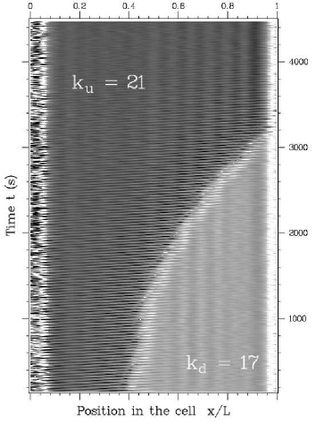
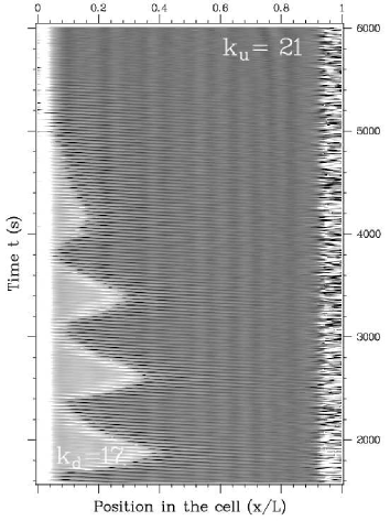
Figure 13: Spatio-temporal diagrams of the spatial phase gradient (local and instantaneous wavenumber) for transients leading to an homogeneous state as the one of Fig. 12a. Initial conditions follow the protocol described in the text, they have been prepared at $t=0$. A dislocation front is slowly advected out of the cell. The modulations grow along $x$ but vanish along $t$: this is the signature of a convective instability regime. Left: right-traveling wave for$\epsilon=0.79$ ($\Delta T=5.44$K), the front position moves monotonically and leads to the final stage presented in Fig. 12a. Right: left-traveling wave $\epsilon=0.78$ ($\Delta T=5.52$K), the front position oscillates before being evacuated at a roughly constant speed.

We call dislocation front the set of spatio-temporal locii where spatio-temporal dislocations occur. For $\epsilon>\epsilon_{\rm m,a}$, the position $x_{F}$ of this object is stationary; Fig. 14 shows the relation between the control parameter and the front position which remains located in the first half of the cell whatever $\epsilon$. Steady dislocation fronts have already been observed for traveling waves in a Taylor-Dean experiment [42]. In general, hysteresis as not been investigated. From the modulation amplitude profiles $A_{\rm mod}(x)$ (Fig. 12c), we also extract the spatial growth rate of the modulations: this quantity will be discussed below togheter with convective and stable regimes (Section 3.4 and Fig. 17).

We pretend those stationary states to be the global modes for the modulational Eckhaus instability. All perturbations leave the structure of those modes unaffected; the front position is always the same at a given value of $\epsilon$. The structure of these global modes is very original: nothing seems to saturate the modulations except the break-up of the underlying wave-pattern, i.e., the abrupt change of the mean-wavenumber downstream the dislocations. Similar patterns have been observed numerically in semi-infinite [43] and closed cells [14]. Like Couairon and Chomaz [43] we observe the nonlinear global threshold and the absolute instability threshold to be identical.

Figure 14: Spatial position $x_{F}$ of the dislocation front for absolutely unstable states vs $\Delta T$. Stable and convectively unstable states without permanent dislocation front are represented as realisations at $x_{F}=L$ (arbitrary choice).

3.3 Convective instability states

For $\Delta T<\Delta T_{\rm m,a}$, dislocation fronts are not observed on asymptotic states. The asymptotic regime (Fig. 12a) is an homogeneous wave, of uniform unmodulated wavenumber $k_{\rm u}\sim 21\!\cdot\!(2\pi/L)$. However, transients obtained after control parameter changes show propagating dislocation fronts (Fig. 13). These fronts are slowly advected out of the channel: those states are convectively unstable states with respect to the modulational Eckhaus instability. Note that the front position can increase monotonically or with an oscillation at a given low frequency. It seems that this oscillation may result from the bouncing of the front on the boundary. Although, there is no possible reflection of the modulation on the boundary because there is not support for a backward traveling modulation on the right-traveling carrier. In both cases, we measured the velocity of the front at the end of the process where the velocity is almost constant. Those moving objects are observed in the small gap between $\epsilon_{\rm m,c}=0.76$ ($\Delta T_{\rm m,c}=5.45$K) and $\epsilon_{\rm m,a}=0.79$ ($\Delta T_{\rm m,a}=5.56$K).

3.3.1 Noisy source states

Due to the special hydrodynamic of the thermocapillary problem, there is another way of observing transients and measuring spatial growth rates. The silicon oil used in the experiments is very volatile and during long experimental runs, the fluid depth in the cell decreases. Of course, we keep working with fluid depth almost constant around $h=1.7$mm, but during some runs $h$ can decrease down to 1.65 mm. For this small depth — small but still within the error-bars we allowed — the boundary emitting waves, acting as a source, becomes larger in space and noisy. This may be interpreted as follows: the system has at the beginning of the run a rather well-fixed wavenumber — around 21.($2\pi/L$) — and wants to keep locked on this value for a given $\epsilon$, even if the fluid depth $h$ decreases; this is only possible if the effective size of the system is reduced by shifting the source from the boundary of the cell to the interior of the cell. This gives an apparently large source because the opposite traveling wave is very damped and almost invisible. The position of the displaced source is not well defined and this may explain the fluctuations observed. Moreover, the source may emit modulations, so we call it a noisy source.

Although hydrodynamic considerations may better explain the exact nature of this source, we only look at it in the present study as a source of modulations over the upstream wavenumber $k_{u}$, the stability of which we are considering. The aim is to study the response of our system under a continuous forcing and such a source provides a convenient forcing. Fig. 15 shows the response of the system to the apparition of a noise source. On Fig. 15, a uniform right-traveling wave is displayed for $t\lesssim 1000$s. At $t\simeq 1000$s, $h$ decreases under a critical value and a source appears near $x/L\simeq 0.1$. Then, modulations are continuously emitted from the source. On Fig. 15 (left) these modulations appear as waves on the local frequency data. The amplitude of this modulation is viewed on Fig. 15 (right) obtained after demodulation of the left diagram: black represents unmodulated waves (zero amplitude) and white represents the maximum modulation level reached. After a complex transient between $t\simeq 1000$s and $t\simeq 4000$s, we observe the modulation amplitude to decay along both spatial and temporal axis. In this case, the basic unmodulated waves are thus stable with respect to the modulations induced by the presence of the noisy source.

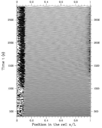
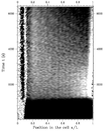
Figure 15: Modulations emitted by a noisy source for $\epsilon=0.70$ ($\Delta T=5.27$K). The noisy source appears at time $t\simeq 1000$s at $x/L\simeq 0.1$. Left: spatio-temporal diagram of the local frequency obtained after using Hilbert demodulation ($400{\rm s}<t<2800{\rm s}$). Right: spatio-temporal diagram obtained after a second demodulation applied on the left-side diagram, showing the amplitude of the modulation ($0<t<6400$s). Before time $t\simeq 1000$s, the right-traveling hydrothermal wave is unmodulated: uniform gray-level for the frequency (left) and black or zero amplitude for the modulation (right). After $t\simeq 1000$s, the wave is modulated. One can see on the amplitude of the modulation (right diagram) that, after a transient ($t\gtrsim 4000$s), the perturbations emitted by the source are spatially and temporally damped: this is illustrated by the darker zone in the upper right part of the image. It is the signature of the hydrothermal wave being stable with respect to modulations.

In Fig. 16 several profiles of the modulation amplitude are presented for various $\epsilon$. Such profiles are extracted at the end of diagrams similar to Fig. 15 (right), i.e., in the asymptotic state where the modulation amplitude decays along time. Again, the amplitude of the frequency modulation is obtained by a second Hilbert transform performed on the local frequency data. We observed that for $\epsilon>\epsilon_{\rm m,c}$ perturbations are spatially amplified whereas they are damped for $\epsilon<\epsilon_{\rm m,c}$.

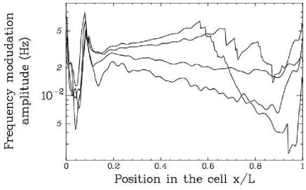
Figure 16: Superposition of several asymptotic profiles of modulation amplitude in the case where a noisy source is present around. The source is on the left ($x=0$) and the waves are right-propagating. Those profiles are extracted at the end of the time series, but still during the transient which may take a very long time to completely relax to zero. (see Fig. 15 ,right). The signal portion just downstream of the source core ($x/L\gtrsim 0.2$) reveals the stability of the modulation. From bottom to top, $\epsilon=0.690$, $0.732$, $0.752$ and $0.765$. For the two lower values of $\epsilon$, the modulations relaxes to zero as they propagate: the unmodulated wave is stable. For the two higher values of $\epsilon$, the modulations are spatially amplified: the unmodulated wave is convectively unstable. The critical value for the transition is $\epsilon_{\rm m,c}=0.758\pm 0.010$ or $\Delta T_{\rm m,c}=(5.45\pm 0.03)$K.

3.4 Stable / convectively unstable transition

For $\epsilon<\epsilon_{\rm m,c}$, asymptotic states are uniform and dislocation fronts do not exist in the absence of forcing. In the presence of forcing by a noisy source, the perturbations are spatially damped as they are advected away from the source (Fig. 15). Close to $\epsilon_{\rm m,c}$ very long transients are often observed. These transient patterns are also slightly modulated; this is illustrated in Fig. 15. Most often, the modulations do not reach the critical amplitude producing dislocations. Asymptotically, the modulation amplitude is decreasing (negative spatial growth rate) along the downstream direction for $\epsilon<\epsilon_{\rm m,c}$, and increasing for $\epsilon>\epsilon_{\rm m,c}$. Anyway, since $\epsilon<\epsilon_{\rm m,a}$, we observe the modulation amplitude to decay along time. On the modulation amplitude image in Fig. 15 (right), a dark corner on the upper right part on the image signs the spatial and temporal damping of the modulation after a long relaxation. The complete relaxation may last much longer than the experimental running time, and those results have to be considered with care. Above $\epsilon_{\rm m,c}$, asymptotic states in the presence of forcing are not uniform but constitute global modes under an external forcing.

On a quantitative point of view, we measured spatial and temporal growth rates of the modulation. We will present these data for the unstable upstream wave-train. The temporal growth rate for modulations in the laboratory frame is negative below $\epsilon_{\rm m,a}$ and positive above. It is also close to zero around the convective transition where very long transient are reported. The spatial growth rate of the upstream $k_{\rm u}$ wave-train for all three regimes is presented on Fig. 17a. It is positive for both unstable states but the slope is seemingly different in the convective and absolute regimes. It is negative below $\epsilon_{\rm m,c}$.

Figure 17: (a) Evolution of the spatial growth rate of the modulation with the control parameter for spontaneously modulated wave patterns, transient ($\circ$) or steady ($\Box$). Linear fits of the three regimes —stable, convective and absolute— are presented. They intersect at $\epsilon_{\rm m,c}$ and $\epsilon_{\rm m,a}$. These data concerns the modulations of the upstream region of the cell whose mean wavenumber is $k_{\rm u}\sim 21\!\cdot\!(2\pi/L)$. Corresponding data for the downstream region are negative while $\Delta T\leq 8$K. (b) Idem for perturbation initiated wave-packets in the stable ($+$) and convectively unstable ($\circ$) regimes. The solid lines recall the fits of (a) to allow quantitative comparisons: the same selection of the growth rate is observed in both cases for the convective regime.

3.5 Perturbed states

In order to test the above description, we perturbed the uniform states by either plunging a thin needle in the convective layer or by dropping a cold or hot droplet of fluid. Two examples are reproduced on Fig. 18. The frequency contents of those perturbations differ from the above reported transients or forced states: the modulation wave-trains contains only a few wavelengths and appears to be advected downstream at roughly the group velocity. All observed perturbations show positive spatial growth rate and negative temporal growth rate in the laboratory frame. The spatial growth rates are presented in Fig. 17b. In the convective regime, the growth rate appears to be selected at the same value than in spontaneous transients or forced states. In the stable regime, however, the data are very dispersed but remain positive.

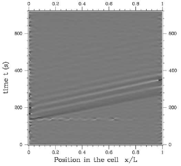
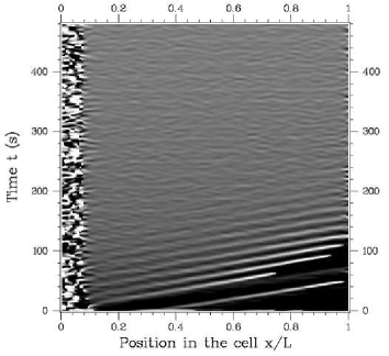
Figure 18: Spatio-temporal diagrams of the local frequency showing the response to an external mechanical perturbation. Left: $\epsilon=0.735$ ($\Delta T$=5.38K); a perturbation is induced at time $t=130$s. Right: $\epsilon=0.764$ ($\Delta T$=5.47K); a perturbation is induced at time $t=0$s. Modulations are spatially growing, but are advected away very quickly. So they disappear after a few 100 seconds.

3.6 Discussion

First, let’s point out that the upstream and downstream wavenumber are incommensurate, and so are the associated frequencies. On Fig. 7, two branches are visible on the frequency data, corresponding to the two different wavenumbers $k_{\rm u}$ and $k_{\rm d}$. The mean ratio between the frequency of $k_{u}$ and $k_{d}$ is $1.130\pm 6.10^{-3}$, i.e., far from any simple rational fraction. This is shown in Fig. 19. We then conclude than those two frequencies are not resonant and that no locking occurs in our system.

Figure 19: Ratio of the frequency in the upstream region by the frequency in the downstream region, versus $\epsilon$. This ratio is almost constant, and its value $1.130\pm 6.10^{-3}$ is far from any simple fraction.

Second, let’s point out that the modulation amplitude $A_{\rm mod}$ never saturates. All observed $A_{\rm mod}$ profiles appear locally exponential along $x$. No non-linear saturation effect is thus observed. The dislocation onset, for a given $A_{\rm mod}\sim|k_{\rm u}-k_{\rm d}|$ is the only limit to exponential growth. This is a strong argument for the Eckhaus instability to behave subcritically in this closed cell. Remember it is supercritical in the annular cell [16] (see I for discussion).

Third, the modulation wave system is a perfect single wave system: reflection of the modulations at the boundaries are irrelevant for there is no possibility for reflected information to travel back to the source without being supported by a counter propagating wave.

The observation facts related above are coherent with the interpretation in terms of convective and absolute instability. The striking point is the positive spatial growth rates for perturbations in the seemingly stable regime below $\epsilon_{\rm m,c}$. As for spontaneously modulated patterns, we would expect those modulation wave-packets to decrease in space exactly as the stable $k_{\rm d}$ wave-trains do in the absolute regime (Fig. 12c).

We may explain this in the following way: Suppose the convective instability is subcritical as suggested previously. Then, above $\epsilon_{\rm m,c}$, the transient evolves on an unstable branch (Fig. 13), close to the absolute branch (Fig. 12b). However, below $\epsilon_{\rm m,c}$, a second unstable branch co-exists, which can be reached only by perturbing the flow: this description can be supported by the schematic Fig. 20 inspired by zero group velocity instabilities. These branches present very different patterns: The upper branch exhibits extended modulations over the whole cell, with slow evolution and, for high enough amplitudes —the generally observed case above $\epsilon_{\rm m,c}$—, dislocation fronts. The lower branch exhibits fast traveling narrow modulation wave-trains and cannot be reached spontaneously by varying $\epsilon$.

This hypothesis can explain the very different aspect of spontaneous and induced transients in the stable regime below $\epsilon_{\rm m,c}$. It is also known that the shape of induced non-linear patterns below subcritical instabilities depends of the forcing amplitude [44], so the dispersion in Fig. 17b may be due to both the effect of amplitude and the presence of two branches.

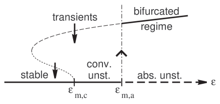
Figure 20: Schematic representation of the observed regimes, based on the usual representation of a subcritical bifurcation with zero group velocity. The control parameter $\epsilon$ is in abscissa, while the ordinate is only qualitative. Solid heavy lines represents the steady states, bifurcated or not, above or below $\epsilon_{\rm m,a}=0.794$K. The thin dashed lines may account for two different transient modes (see text).

Another observation of the convective branch is intriguing. We report in Fig. 21 the asymptotic velocity of the dislocation fronts between $\epsilon_{\rm m,c}$ and $\epsilon_{\rm m,a}$, i.e., the tangent to the space-time trajectory when the front quits the cell as on Fig. 13. The observation is surprising: the closer the absolute instability onset, the faster the front moves! And then jumps below zero above $\Delta T_{\rm m,a}$. A contrario, around $\epsilon_{\rm m,c}$, the front velocity is zero, leading to infinitely long transients, i.e., temporal marginality. This quantifies the experimental complexity of carrying the experiment around this point.

What is the meaning of the velocity jump at $\epsilon_{\rm m,a}$? Is the convective/absolute transition also subcritical? Probably it is: while our protocol did not allow to explore all branches by varying $\epsilon$ up and down from one state to another, a test have been made to transit directly from an absolute state to a stable state just below $\epsilon_{\rm m,c}$: the absolute modulation profile remains fixed in the cell. This can be due either to hysteresis, either to the vanishing front velocity… which makes the system marginal in this region. This point would need to be addressed with an improved experimental device.

Figure 21: Front velocity around the convective/absolute transition. The circles ($\circ$) show the velocity of dislocation fronts in transient convective regimes below $\epsilon_{\rm m,a}$. The (negative) velocities of transient modulation fronts invading the cell from downstream, above $\epsilon_{\rm m,a}$, are shown by squares ($\Box$). For comparison, the group velocity is $0.90{\rm mm.s^{-1}}$.

Let’s note that for higher $\epsilon$ values, the front position $x_{F}(t)$ exhibits chaotic behaviors and can thus be viewed as the order parameter for the modulational instability up to the transition to spatio-temporal chaos. An example of disordered state is presented on Fig. 22 which suggest that the spatio-temporal behavior can be described using this front as a dynamical system.

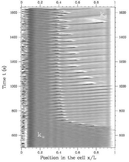
Figure 22: Transient for $\epsilon=1.74$ with $k_{u}=19\cdot(2\pi/L)=0.65$mm^-1 and $k_{d}=16\cdot(2\pi/L)=0.56$mm^-1. A period doubling occurs for the modulation front: one modulation over two explodes in a dislocation forming a first dislocation front in space-time, then one modulation over 4 explodes forming another dislocations front, then one over 8 forms another front, and so on until all those dislocations fronts merge together leaving a state in which $k_{u}$ is absolutely unstable.

Last but not least, modulations in the rectangle can be connected to modulations in the annulus described in section LABEL:sec:annulus of I. First, in periodic boundary conditions, the Eckhaus secondary instability is supercritical for wavenumbers close to the critical one, whereas it is rather subcritical far from the critical wavenumber $k_{\rm c}$. This is confirmed by observations in non-periodical boundary conditions: the selected wavenumbers are far from $k_{\rm c}$ in the rectangle and the modulational instability is subcritical. This opens the following question: can the observed modulations in the rectangle be described as modulated amplitude waves (MAWs) [45, 46, 47] ? Such modulations have already been seen by [2, 3, 5]. As pointed out before, modulated waves in the rectangle are not saturated, neither should be corresponding MAWs; moreover, the spectral richness of the modulations is weak in the rectangle: modulations are almost monochromatic. So, speaking of MAWs, we are facing solutions of the CGL equation that connect two non-saturated modulated waves.

4 Sources and sinks in the annulus

Coming back to the annulus will allow us to show that the convective/absolute transitions advocated for in the rectangle is also relevant in periodic boundary conditions, when the Galilean invariance is broken due to the presence of both right- and left-traveling waves. The interpretation of bifurcations in the rectangle in terms of convective/absolute transitions is then reinforced.

4.1 Obtaining source/sink pairs

Let us describe how patterns form when $\epsilon$ is rapidly increased from a negative value to a supercritical value $\epsilon_{\rm f}$; describing those transients allow us to distinguish between different behaviors. In all such experiments, the waves first appear in small patches at several places in the cell. The envelopes of those patches propagate at group velocity while their spatial extension increase. After a short transient, waves have invaded all the cell but sources and sinks are presents which are reminiscent of the boundaries of the initial patches. The number of initial patches, and so the number of sources and sinks depends on the time derivative of the ramp in $\epsilon$ leading to $\epsilon_{\rm f}$ : the faster the control parameter is varied across the threshold of waves, the more sources/sinks pairs are present in the cell; a typical realization shows two or three pairs. Quasi-static variations of $\epsilon$ shows at least one pair.

This first ”invasion” time is followed by a second transient regime where sources and sinks interact. Fig. 23 presents a typical competition leading to the annihilation of two source/sink pairs. For this experiment, we start from a supercritical value $\epsilon=0.14$ ($\Delta T=3.52$K) and a single right-traveling wave and then reduce the control parameter by switching off the electrical heating of the inner block. So $\Delta T$ decreases and the right-traveling wave disappear as the onset is crossed from above. As soon as the wave disappear, we switch the heating on again. Waves reappears in four different patches forming two sources and two sinks. Then, after a 5 minutes transient, the left wave remains alone.

A nice observation is done by looking around the value $\epsilon_{\rm a}$. If the operating value $\epsilon_{\rm f}$ is close to 0, all pairs annihilate within the transient and the asymptotic pattern is always a single homogeneous traveling wave. For $0<\epsilon_{\rm f}<\epsilon_{\rm a}=0.18$, no source/sink pattern has been seen asymptotically. In contrast, when $\epsilon_{\rm f}>\epsilon_{\rm a}$, i.e., the ending value of the imposed control parameter is highly supercritical, it is possible —but not mandatory— to have a source/sink pattern frozen on long times. We have observed that the higher $\epsilon_{\rm f}$ is, the easier source/sink states are easily frozen [16]. For $\epsilon_{\rm f}>\epsilon_{\rm a}$, we have observed some realizations in which sources and sinks are present after times much longer than the diffusion time.

So in the annular experiment, sources and sinks have been observed during transients for all possible values of $\epsilon$. But a striking result is that the couples of sources and sinks are always unstable below $\epsilon<\epsilon_{\rm a}=0.18$; in that case, all source/sink pair collapse and only an homogeneous single wave subsists. In contrast, sources and sinks have been observed in a stable way for $\epsilon>\epsilon_{\rm a}$, i.e., at least such a pair lasts as long as the experiment is performed.

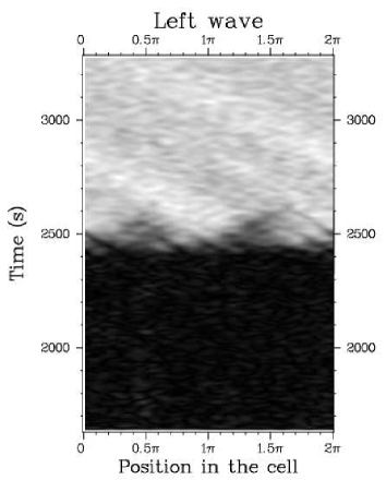
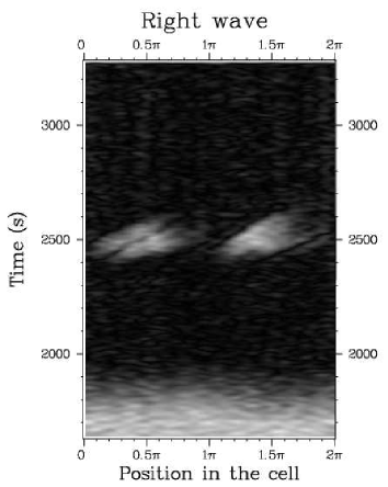
Figure 23: Spatio-temporal diagrams of the local amplitude showing the initial competition between right- and left-propagating waves in the annulus. Left : amplitude of left-traveling waves. Right : amplitude of right-traveling waves. The gray scale is proportional to the amplitude (increasing from black to white). $\Delta T$ is increased slowly from a (slightly) subcritical value to 3.60 K ($\epsilon_{\rm f}=0.16$). Two couples of source/sink appear quickly at time $t=2400$s; then they interact and only a single wave remains after time $t=2600$s. Note that initially (before $t=1800$s), only the right-traveling wave is present, and after $t=2700$s, only the left-traveling wave is present; on that remaining left wave, a transient modulation is present.

4.2 Convective/absolute onset in the annulus

Below $\epsilon_{\rm a}$, source/sink couples are unstable in the sense that they collapse together, but sources can also be qualified as unstable because they emit modulations. Those modulations are also present close to the onset of waves.

It has been theoretically and numerically [9, 48] established that stables sources only exists in a 1D-periodical geometry when the control parameter $\epsilon$ is above $\epsilon_{\rm abs}$, i.e., when the instability is absolute. This may be understood remembering that in the convective regime, the wave-system acts as a noise amplifier. The two different regimes for the sources are to be discerned: below $\epsilon_{\rm abs}$, sources are noisy and their width is large; above $\epsilon_{\rm abs}$, sources selection a wavenumber and have a smaller spatial extend.

Measurements of the source width have been performed recently in a very long rectangular geometry [33, 49] leading to a nice confirmation of this transition. Here, we use the qualitative observation of stable sources above $\epsilon_{\rm a}=0.18$ and the disappearance of all sources below $\epsilon_{\rm a}$ to confirm that $\epsilon_{\rm abs}=0.18$ in the annulus. Using expression of $\epsilon_{\rm abs}$ in Eq. (2), and assuming that the parameters involved are the same in both rectangle and annular geometry, we are confident that the overall description using convective/absolute transition for the onset shift in the rectangle is relevant.

4.3 Discussion

As previously said, modulations are emitted by the sources, even if $\epsilon$ is close to 0. Moreover, when a single traveling wave is finally produced by the collapse of the last sink within the last source, modulations are also emitted. So the single unmodulated uniform traveling wave pattern appears always after a transient in which initial modulations are present but damped. This transient is studied in I (section LABEL:sec:mwdamped and Fig. LABEL:fig:mwdamped). The detailed study of modulations emitted by the sources remains to be done, but one can expect that sources in the annulus behave like the one in the rectangle. For example, if their position is not well fixed as it is the case of noisy sources in the rectangle (section 3.3.1), it may explain the same emission of modulations.

As studied in Refs [9, 50] the effect of the group velocity is also a key point for a better understanding of traveling wave systems in both non-periodic and periodic geometries. Other parameters such as the complex coupling coefficient ($\lambda+i\mu$ in Eq. 1) should also be tracked for influence on the observed patterns in both geometries, thus suggesting that the complex Ginzburg-Landau equations cannot be only described using simply two parameters ($c_{1}$ and $c_{2}$ in Eq. 1).

Conclusion

Owing to their apparition via a supercritical instability with finite frequency, finite wavenumber and finite group velocity, hydrothermal waves were previously shown to be very well modelized by an amplitude equation of the complex Ginzburg-Landau type (paper I). In the present article, we used a one-dimensional hydrothermal wave system as an experimental expression of the one dimensional CGL equation or of a system of coupled one-dimensional CGL equations, to explore the effect of the boundary conditions.

We have presented the global mode appearing in a rectangular box at the absolute instability threshold for hydrothermal traveling waves. Qualitative and quantitative comparisons have been performed to distinguish from the case of a reflection-controlled global mode. The relevance of the convective/absolute distinction was demonstrated by accurate comparison of threshold values and critical behaviors of the order parameters. Those measurements have revealed that the transition is fully non-linear in the sense of Chomaz and Couairon [26] and is well connected to the predictions of [14] for a single wave pattern.

For higher control parameter values in the rectangle bounded cell, we observe a quasi one-directional traveling-pattern which undergoes an Eckhaus secondary instability leading to traveling modulations. These modulated patterns behave as non-linear fronts whose dynamics reveals convective and absolute regimes as well [27, 18]. Thus we have observed both stable/convective and convective/absolute transitions for the modulational instability. The stable/convective transition is subcritical and is characterized by zero spatial growth rate for the modulation, together with zero advection velocity of the modulated pattern, which can be viewed as spatial and temporal marginality. The convective/absolute transition is characterized by the dynamics of dislocation fronts. According to front velocity data, we suggest this transition to be subcritical as well which qualitatively differs from the case of the annulus. This question deserves a theoretical support which remains yet, as far as we know, unexplored.

Finite group velocity in the presence of boundaries, leading to the transition from convective to absolute, are linked with important qualitative and quantitative changes of the global structure of the wave patterns in rectangular geometry. We showed that this is also true in the annulus where sources emitting waves are very sensitive to the convective or absolute nature of the primary waves. The description of one-dimensional hydrothermal waves using Ginzburg-Landau equations appears to be very complete and satisfactory. One may expect even more connections with future theoretical work on these equations.

References

- [1] N. Garnier, A. Chiffaudel, F. Daviaud, and A. Prigent. Nonlinear dynamics of waves and modulated waves in 1D thermocapillary flows. I: General presentation and periodic solutions. Companion paper, part 1, 2002.
- [2] P. Kolodner. Extended states of nonlinear traveling-wave convection. I. The Eckhaus instability. Phys. Rev. A, 46:6431, 1992.
- [3] G.W. Baxter, K.D. Eaton, and C.M. Surko. Eckhaus instability for traveling waves. Phys.Rev. A, 46:R1735, 1992.
- [4] B. Janiaud, A. Pumir, D. Bensimon, V. Croquette, H. Richter, and L. Kramer. Eckhaus instability for traveling waves. Physica D, 55:269, 1992.
- [5] Y. Liu and R.E. Ecke. Nonlinear traveling waves in rotating Rayleigh-Bénard convection: Stability boundaries and phase diffusion. Phys. Rev. E, 59:4091, 1999.
- [6] T. Leweke and M. Provansal. The flow behind rings: bluff body wakes without end effects. J. Fluid Mech., 288:265, 1995.
- [7] R.J. Deissler. Noise-sustained structure, intermittency and the Ginzburg-Landau equation. J. Stat. Phys., 40:371, 1985.
- [8] A. Couairon and J.M. Chomaz. Primary and secondary nonlinear global instability. Physica D, 132:428, 1999.
- [9] M. van Hecke, C. Storm, and W. van Saarloos. Sources, sinks and wavenumber selection in coupled CGL equations and experimental implications for counter-propagating wave systems. Physica D, 134:1, 1999.
- [10] V. Croquette and H. Williams. Nonlinear waves of the oscillatory instability on finite convective rolls. Physica D, 37:300, 1989.
- [11] A. Chiffaudel, B. Perrin, and S. Fauve. Spatiotemporal dynamics of oscillatory convection at low Prandtl number: waves and defects. Phys. Rev. A, 39:2761, 1989.
- [12] M.C. Cross. Structure of nonlinear traveling-wave states in finite geometries. Phys. Rev. A, 38:3593, 1988.
- [13] M.C. Cross and E.Y. Kuo. One dimensional spatial structure near a Hopf bifurcation at finite wavenumber. Physica D, 59:90, 1992.
- [14] S.M. Tobias, M.R.E. Proctor, and E. Knobloch. Convective and absolute instabilities of fluid flows in finite geometry. Physica D, 113:43, 1998.
- [15] P. Gondret, P. Ern, L. Meignin, and M. Rabaud. Experimental evidence of a nonlinear transition from convective to absolute instability. Phys. Rev. Lett., 82:1442, 1999.
- [16] N. Mukolobwiez, A. Chiffaudel, and F. Daviaud. Supercritical Eckhaus instability for surface-tension-driven hydrothermal waves. Phys. Rev. Lett., 80:4661, 1998.
- [17] N. Garnier and A. Chiffaudel. Nonlinear transition to a global mode for traveling-wave instability in a finite box. Phys. Rev. Lett., 86:75, 2001.
- [18] N. Garnier and A. Chiffaudel. Convective and absolute Eckhaus instability leading to modulated waves in a finite box. Phys. Rev. Lett., 88:134501, 2002.
- [19] J. Burguete, N. Mukolobwiez, F. Daviaud, N. Garnier, and A. Chiffaudel. Buoyant-thermocapillary instabilities in extended liquid layers subjected to a horizontal temperature gradient. Phys. Fluids, 13:2773, 2001.
- [20] M.C. Cross and P.C. Hohenberg. Pattern formation outside of equilibrium. Rev. Mod. Phys., 65:851, 1993.
- [21] I. Aranson and L. Kramer. The world of the complex Ginzburg-Landau equation. Rev. Mod. Phys., 74:99, 2002.
- [22] N. Garnier. Ondes non-linéaires à une et deux dimensions dans une mince couche de fluide. PhD. thesis, University Paris 7 Denis Diderot, 2000.
- [23] N. Garnier and C. Normand. Effects of curvature on hydrothermal waves instability of radial thermocapillary flows. Comptes-rendus de l’Académie des Sciences, Serie IV, 2(8):1227, 2001.
- [24] E. Kaplan and V. Steinberg. Measurement of reflection of traveling waves near the onset of binary-fluid convection. Phys. Rev. E, 48:R661, 1993.
- [25] J. Fineberg, V. Steinberg, and P. Kolodner. Weakly nonlinear states as propagating fronts in convecting binary mixtures. Phys. Rev. A, 41:5743, 1990.
- [26] J.M. Chomaz and A. Couairon. Against the wind. Phys. Fluids, 11:2977, 1999.
- [27] N. Garnier and A. Chiffaudel. Caractères absolu et convectif de l’instabilité en ondes hydrothermales. In Y. Pomeau and R. Ribotta, editors, Troisième rencontre du non-linéaire, Paris 9-10 mars 2000, pages 233–238. Editions Paris Onze, 2000.
- [28] J. Priede and G. Gerbeth. Convective, absolute, and global instabilities of thermocapillary-buoyancy convection in extended layers. Phys. Rev. E, 56(4):4187, 1997.
- [29] M.A. Pelacho, A .Garcimartin, and J. Burguete. Local Marangoni number at the onset of hydrothermal waves. Phys. Rev. E, 62:477, 2000.
- [30] J.M. Vince and M. Dubois. Critical properties of convective waves in a one-dimensional system. Physica D, 102:93, 1997.
- [31] P. Huerre and P. Monkewitz. Local and global instabilities in spatially developing flows. Ann. Rev. of Fluid Mech., 22:473, 1990.
- [32] B. Sandstede and A. Scheel. Absolute versus convective instability of spiral waves. Physica D, 145:233, 2000.
- [33] L. Pastur, M. T. Westra, and W. van De Water. Sources and sinks in 1D travelling waves. Submitted for this issue of Physica D., 2002.
- [34] M.C. Cross. Traveling and standing waves in binary-fluid convection in finite geometries. Phys. Rev. Lett., 57:2935, 1986.
- [35] C. Martel and J. Vega. Finite size effects near the onset of the oscillatory instability. Nonlinearity, 9:1129, 1996.
- [36] C. Martel and J. Vega. Dynamics of a hyperbolic system that applies at the onset of the oscillatory instability. Nonlinearity, 11:105, 1998.
- [37] L. Tuckerman and D. Barkley. Bifurcation analysis of the Eckhaus instability. Physica D, 46:57, 1990.
- [38] L. Tuckerman and D. Barkley. Comment on “bifurcation structure and the Eckhaus instability”. Phys. Rev. Lett., 67:1051, 1991.
- [39] A. Weber, L. Kramer, I. S. Aranson, and L. Aranson. Stability limits of traveling waves and the transition to spatiotemporal chaos in the complex Ginzburg-Landau equation. Physica D, 61:279–283, 1992.
- [40] I. S. Aranson, L. Aranson, L. Kramer, and A. Weber. Stability limits of spirals and traveling waves in nonequilibrium media. Physical Review A, 46:R2992–2995, 1992.
- [41] W. Eckhaus. Studies in Nonlinear Stability Theory. Springer, 1965.
- [42] P. Bot and I. Mutabazi. Dynamics of spatio-temporal defects in the Taylor-Dean system. Eur. Phys. J. B, 13:141, 2000.
- [43] A. Couairon and J.M. Chomaz. Primary and secondary nonlinear global instability. Physica D, 132:428, 1999.
- [44] S. Bottin and H. Chaté. Statistical analysis of the transition to turbulence in plane Couette flow. Eur. Phys. J. B, 6:143, 1998.
- [45] L. Brusch, A. Torcini, M. van Hecke, M.G. Zimmermann, and M. Bär. Modulated amplitude waves and defect formation in the one-dimensional Ginzburg-Landau equation. Physica D, 160:127, 2001.
- [46] L. Brusch, A. Torcini, and M. Bär. Nonlinear analysis of the Eckhaus instability modulated amplitude waves and phase chaos with non-zero average phase gradient. Submitted for this issue of Physica D, 2002.
- [47] M. van Hecke. Coherent and incoherent structures in systems described by the 1D CGLE: experiments and identification. Submitted for this issue of Physica D, 2002.
- [48] U. Ebert and W. van Saarloos. Front propagation into unstable states: universal algebraic convergence towards uniformly translating pulled fronts. Physica D, 146:1, 2000.
- [49] In reference [33], the geometry is non-periodical, but very extended. This allows to conjecture that and so that waves exist for .
- [50] H. Riecke and L. Kramer. The stability of standing waves with small group velocity. Physica D, 137:124, 2000.