Mean effects of turbulence on elliptic instability in fluids

Abstract

Elliptic instability in fluids is discussed in the context of the Lagrangian-averaged Navier-Stokes-alpha (LANS$-\alpha$) turbulence model. This model preserves the Craik-Criminale (CC) family of solutions consisting of a columnar eddy and a Kelvin wave. The LANS$-\alpha$ model is shown to preserve the elliptic instability for the inviscid case. However, the model shifts the critical stability angle. This shift increases (resp. decreases) the maximum growth rate for long (resp. short) waves. It also introduces a band of stable CC solutions for short waves.

Elliptic, or tilting, instability is a fundamental phenomenon in fluids that results from parametric resonance. This is the mechanism by which vortex stretching creates three dimensional instabilities in swirling two dimensional flows. Specifically, the energy in an elliptical columnar eddy may be transferred to a propagating Kelvin wave kelvin by this mechanism. A breakthrough in the study of this problem occurred when Craik & Criminale craik:crim:86 showed that superposing a columnar eddy and a Kelvin wave yields an exact solution of the Euler equations. Thus, the elliptical instability can be treated as a modulation of the Craik-Crimale (CC) family of solutions by using Floquet analysis as was first done by Bayly bayly:86 . The history of discovery and rediscovery of elliptic instability in laminar fluids is reviewed by Kerswell ker:02 . Here we address the mean effects of turbulence on the elliptic instability. The CC family of superposed solutions is preserved by the closure model we shall consider. For this model, turbulence is shown to enhance the growth rates of elliptic instability for Kelvin wavelengths that are longer than the turbulence correlation length. Conversely, turbulence is found to suppress elliptic instability at the shorter wavelengths and to create a band of stable CC flows with nonzero eccentricities.

The turbulence model we shall consider is the Lagrangian-averaged Navier-Stokes-alpha (LANS$-\alpha$) model chen:foias:holm:olson:titi:wynne , whose equations are:

$$\frac{\partial{{\mathbf{v}}}}{\partial t}+({{\mathbf{u}}}\cdot{\nabla}){\mathbf{v}}+{(\nabla u)^{T}}\cdot{{\mathbf{v}}}\\ +\nabla\left(p-\tfrac{1}{2}|{\mathbf{u}}|^{2}-\tfrac{1}{2}\alpha^{2}|\nabla{\mathbf{u}}|^{2}\right)=\nu\Delta{\mathbf{v}}$$ (1)

together with ${\nabla}\cdot{{\mathbf{u}}}=0$. In this model, the mean fluid velocity $\mathbf{u}$ is related to the mean momentum $\mathbf{v}$ via the Helmholtz operator $(1-\alpha^{2}\Delta)$ as ${\mathbf{v}}={\mathbf{u}}-\alpha^{2}\Delta{\mathbf{u}}$. This Helmholtz filtering of the fluid velocity introduces the length scale $\alpha$ as a parameter in the model. The LANS$-\alpha$ model preserves the fundamental transport theorems for circulation and vorticity dynamics of the NS equations. Direct numerical simulations of the LANS$-\alpha$ model for forced homogeneous turbulence show it to be considerably less computationally intensive than the exact NS equations while preserving essentially the same behavior as NS at length scales larger than alpha chen:holm:mar:zha:99 . The unforced, inviscid Euler$-\alpha$ form of these equations first appeared in the context of averaged fluid models holm:mar:rat . The basic properties of the LANS$-\alpha$ model, its comparison with experiment, and its early development are reviewed in Ref. foias:holm:titi:01, . See also Refs. newalpha, for additional results for this model. As discussed in Ref. holm:mar:rat the LANS$-\alpha$ turbulence equations formally coincide in the inviscid limit with a classic rheological model known as the 2nd-grade fluid grade2 . Thus, the present results for the inviscid elliptic instability apply to both the LANS$-\alpha$ turbulence model and to rheology of 2nd-grade fluids.

We construct an exact solution to Eq. (1) with zero divergence of the form ${\mathbf{u}}_{0}({\mathbf{x}},t)={\mathcal{S}}(t){\mathbf{x}}+{\mathbf{U}}(t)$, where ${\mathcal{S}}{\mathbf{x}}$ is the action of the matrix ${\mathcal{S}}$ on the vector ${\mathbf{x}}=[x,y,z]^{T}$ from the left. The matrix ${\mathcal{S}}$ is a time dependent matrix with zero trace such that $d{\mathcal{S}}/dt+{\mathcal{S}}^{2}={\mathcal{M}}(t)$, where ${\mathcal{M}}(t)$ is a symmetric matrix which contains the contributions of ${\mathbf{U}}(t)$. The corresponding pressure $p_{0}$ is obtained from ${\mathcal{M}}(t)$; see Ref. craik:crim:86, for details. We nondimensionalize the system using the variables ${\mathbf{x}}^{\prime}={\mathbf{x}}/l$, $t^{\prime}=\omega t$, ${\mathbf{u}}^{\prime}={\mathbf{u}}/\omega l$, ${\mathbf{v}}^{\prime}={\mathbf{v}}/\omega l$, $\alpha^{\prime}=\alpha/\sqrt{l}$, where $l$ is a typical length scale and $\omega=\tfrac{1}{2}|\nabla\times{\mathbf{u}}_{0}|$. The resulting equation with the prime notation suppressed is Eq. (1) with $\nu$ replaced by $\nu/\omega$. We construct a second solution to Eq. (1) of the form ${\mathbf{u}}_{0}+{\mathbf{u}}_{1}$ with corresponding pressure $p_{0}+p_{1}$, where

$${\mathbf{u}}_{1} =\mu{\mathbf{a}}(t)\sin(\beta\psi({\mathbf{x}},t)),$$ (2)

$$\begin{split}p_{1}&=\mu\hat{p}_{11}(t)\cos(\beta\psi({\mathbf{x}},t))\\ &\phantom{XXXXXXX}+\mu^{2}\hat{p}_{12}(t)\cos^{2}(\beta\psi({\mathbf{x}},t)),\end{split}$$ (3)

$\psi({\mathbf{x}},t)={{\mathbf{k}}(t)}\cdot{{\mathbf{x}}}+g(t)$, and $\mu$ and $\beta$ are scaling factors so that we can choose the initial conditions $|{\mathbf{a}}(0)|=1$ and $|{\mathbf{k}}(0)|=1$. The unknown phase $\psi({\mathbf{x}},t)$ and the amplitudes ${\mathbf{a}}(t)$, $\hat{p}_{11}(t)$, and $\hat{p}_{12}(t)$ are to be determined. Such flows which are the sum of a ‘base flow’ ${\mathbf{u}}_{0}$ and a ‘disturbance’ ${\mathbf{u}}_{1}$ are called $\alpha$-CC flows. The incompressibility condition gives

$${{\mathbf{a}}}\cdot{{\mathbf{k}}}=0.$$ (4)

The evolution equations for the amplitudes and phase are

$$(\partial_{t}+{{\mathcal{S}}{\mathbf{x}}}\cdot{\nabla})\psi+{{\mathbf{U}}}\cdot{{\mathbf{k}}} =0,$$ (5)

$$\begin{split}(\partial_{t}+{{\mathcal{S}}{\mathbf{x}}}\cdot{\nabla})((1+\Gamma){\mathbf{a}})+\Gamma&{\mathcal{S}}^{T}{\mathbf{a}}+{\mathcal{S}}{\mathbf{a}}\\ -(\beta\hat{p}_{11}-\beta^{2}\alpha^{2}{{\mathbf{a}}}\cdot{{\mathcal{S}}{\mathbf{k}}}){\mathbf{k}}&=-\frac{(1+\Gamma)\nu\beta^{2}}{\omega}|{\mathbf{k}}|^{2}{\mathbf{a}},\end{split}$$ (6)

$$\hat{p}_{12}-\Gamma|{\mathbf{a}}|^{2} =0.$$ (7)

Here $\Gamma=\alpha^{2}\beta^{2}|{\mathbf{k}}|^{2}$. Note that the amplitude scaling $\mu$ is immaterial. The parameter $\alpha$ couples various terms throughout the system. Moreover, this coupling in $\alpha$ appears only in the combination $\Gamma$, which is proportional to wavenumber-squared. Consequently, this coupling affects the high wavenumber behavior of the solution for $\alpha\neq 0$. Equation (5) states that the phase is advected with the base flow. Only two free parameters remain ($\Gamma$ and $E_{\omega}$) upon introducing the vorticity based Ekman number $E_{\omega}=\nu\beta^{2}/\omega$. Without loss of generality, we set $\partial g/\partial t+{{\mathbf{k}}}\cdot{{\mathbf{U}}}=0$. Denoting the material derivative as ${\mathrm{d}_{t}}=(\partial_{t}+{{\mathcal{S}}{\mathbf{x}}}\cdot{\nabla})$ and taking the gradient of Eq. (5) reduces Eqs. (5)-(6) to a system of ordinary differential equations:

$$\frac{\mathrm{d}{{\mathbf{k}}}}{\mathrm{d}t}+{\mathcal{S}}^{T}{\mathbf{k}} =0,$$ (8)

$$\begin{split}\frac{\mathrm{d}{((1+\Gamma){\mathbf{a}})}}{\mathrm{d}t}+(1+\Gamma){\mathcal{S}}^{T}{\mathbf{a}}&\\ +2\varpi\times{\mathbf{a}}-\tilde{P}{\mathbf{k}}&=-(1+\Gamma)E_{\omega}|{\mathbf{k}}|^{2}{\mathbf{a}},\end{split}$$ (9)

where $\tilde{P}$ is the coefficient of ${\mathbf{k}}$ in Eq. (6), $\varpi=\tfrac{1}{2}\nabla\times{\mathbf{u}}_{0}$ is the (normalized) vorticity of the base flow and $({\mathcal{S}}-{\mathcal{S}}^{T}){\mathbf{a}}=2\varpi\times{\mathbf{a}}$. We eliminate the pressure term by taking the dot product of Eq. (9) with ${\mathbf{k}}$ and by using ${{\mathrm{d}}{\mathbf{a}}/{\mathrm{d}t}}\cdot{{\mathbf{k}}}=-{{\mathbf{a}}}\cdot{{\mathrm{d}}{\mathbf{k}}/{\mathrm{d}t}}={{\mathcal{S}}{\mathbf{a}}}\cdot{{\mathbf{k}}}$, the first of which follows from Eq. (4) and the second from Eq. (8):

$$\tilde{P}=\frac{1}{|{\mathbf{k}}|^{2}}\Big{\{}(1+\Gamma){({\mathcal{S}}+{\mathcal{S}}^{T}){\mathbf{a}}}\cdot{{\mathbf{k}}}+2{\varpi\times{\mathbf{a}}}\cdot{{\mathbf{k}}}\Big{\}}.$$ (10)

In summary, we have obtained a new exact incompressible solution to Eq. (1). The variables are amplitude ${\mathbf{a}}(t)$ and wave vector ${\mathbf{k}}(t)$. Once these are determined, the pressure terms follow from Eqs. (7) and (10). Note that ${\mathbf{u}}_{0}$ and ${\mathbf{u}}_{0}+{\mathbf{u}}_{1}$ are exact solutions to the nonlinear equations, but ${\mathbf{u}}_{1}$ by itself is only a solution to Eq. (1) linearized about ${\mathbf{u}}_{0}$. The construction described above also can be applied to Eq. (1) expressed in a rotating coordinate system in which an $\alpha$-CC flow can still be found. The effects of rotation will be discussed elsewhere. Finally, we emphasize that the operator ${\mathrm{d}}/{\mathrm{d}t}+S^{T}$ acting on a vector represents the complete time derivative of that quantity in a Galilean frame moving with ${\mathbf{u}}_{0}$.

Insight into the dynamics of the problem can be gained by examining Eq. (9) in the asymptotic regimes $\Gamma\ll 1$ and $\Gamma\gg 1$, where $\Gamma=\alpha^{2}\beta^{2}|{\mathbf{k}}|^{2}$. (We assume that $|{\mathbf{k}}(t)|$ remains bounded and never vanishes.) For $\Gamma\ll 1$, Eq. (9) becomes

$$\frac{\mathrm{d}{{\mathbf{a}}}}{\mathrm{d}t}+{\mathcal{S}}^{T}{\mathbf{a}}=-E_{\omega}|{\mathbf{k}}|^{2}{\mathbf{a}}-2\varpi\times{\mathbf{a}}+\frac{2{{\mathcal{S}}{\mathbf{a}}}\cdot{{\mathbf{k}}}}{|{\mathbf{k}}|^{2}}{\mathbf{k}}\\ +\Gamma\left(2\varpi\times{\mathbf{a}}+\frac{2}{|{\mathbf{k}}|^{2}}\left\{({{\mathcal{S}}{\mathbf{k}}}\cdot{{\mathbf{k}}}){\mathbf{a}}-({\varpi\times{\mathbf{a}}}\cdot{{\mathbf{k}}}){\mathbf{k}}\right\}\right)\\ +O\left(\Gamma^{2}\right).$$ (11)

Combined with Eq. (8), this equation preserves ${{\mathbf{a}}}\cdot{{\mathbf{k}}}=0$ at each order. The $O(1)$ term in the above equation is exactly the expression for the amplitude of the modulated traveling wave in the CC flow for the classical Euler and NS equations. This, of course, is expected since Eq. (1) reduces to the NS equations for $\alpha=0$. Thus, to leading order, the amplitude decays with viscosity, stretches with the base shear and rigidly rotates with the vorticity of the base flow. For $\Gamma\gg 1$, Eq. (9) becomes

$$\frac{\mathrm{d}{{\mathbf{a}}}}{\mathrm{d}t}+{\mathcal{S}}^{T}{\mathbf{a}}=-E_{\omega}|{\mathbf{k}}|^{2}{\mathbf{a}}+\frac{2{{\mathcal{S}}{\mathbf{a}}}\cdot{{\mathbf{k}}}}{|{\mathbf{k}}|^{2}}{\mathbf{k}}\\ +\frac{2}{|{\mathbf{k}}|^{2}}\left\{({{\mathcal{S}}{\mathbf{k}}}\cdot{{\mathbf{k}}}){\mathbf{a}}-({\varpi\times{\mathbf{a}}}\cdot{{\mathbf{k}}}){\mathbf{k}}\right\}+O\left(\frac{1}{\Gamma}\right).$$ (12)

Again, this equation preserves ${{\mathbf{a}}}\cdot{{\mathbf{k}}}=0$ at each order Thus, as $\Gamma\to\infty$ (corresponding to either $\alpha\to\infty$ or $\beta\to\infty$), the amplitude no longer rigidly rotates with the vorticity of the base flow.

As an example, we examine the stability of a rotating column of fluid with elliptic streamlines whose foci lie on the $y$-axis and vorticity $\varpi=\omega{\mathbf{\hat{e}}_{z}}$:

$${\mathbf{u}}_{0}=\omega L{\mathbf{x}},\quad L=\begin{pmatrix}0&-1+\gamma&0\\ 1+\gamma&0&0\\ 0&0&0\end{pmatrix}.$$ (13)

Here, $0\leq\gamma<1$ is the eccentricity of the ellipses, and the pressure is $p_{0}=\tfrac{1}{2}\omega^{2}(1-\gamma^{2})(x^{2}+y^{2})$. Equation (8) with ${\mathcal{S}}=L$ is analytically solvable:

$${\mathbf{k}}=[\sin\theta\cos(t\sqrt{1-\gamma^{2}}),\\ \kappa\sin\theta\sin(t\sqrt{1-\gamma^{2}}),\cos\theta]^{T}$$ (14)

where $\kappa^{2}=(1-\gamma)/(1+\gamma)$ and $\theta$ is the polar angle that ${\mathbf{k}}$ makes with the axis of rotation. In summary, we have a four parameter problem in $\Gamma$, $E_{\omega}$, $\gamma$, and $\theta$. Eq. (9) has the form ${\mathrm{d}}{\mathbf{a}}/{\mathrm{d}t}={\mathcal{N}}(t){\mathbf{a}}$, where the elements of the matrix ${\mathcal{N}}(t)$ are periodic with period $\tau=2\pi/\sqrt{1-\gamma^{2}}$. Therefore, the system can be analyzed numerically using Floquet theory yaku:star:76 . We compute the monodromy matrix ${\mathcal{P}}$, that is, the fundamental solution matrix with identity initial condition evaluated at $t=\tau$. Equation (9) will have exponentially growing solutions if $\max_{i}|\Re(\rho_{i})|>1$, where $\rho_{i},i=1,2,3$ are the eigenvalues of ${\mathcal{P}}$, with corresponding Lyapunov-like growth rates given by

$$\sigma=\frac{1}{\tau}\ln\{\max_{i}|\Re(\rho_{i})|\}.$$ (15)

Thus, we can simulate numerically the solution to Eq. (9) over one period and indisputably determine the exponential growth rates. We can be certain that at least one of the eigenvalues will always be unity because of the incompressibility condition (4) and that the remaining two eigenvalues appear as complex conjugates on the unit circle or as real valued reciprocals of each other.

The present investigation considers the case of inviscid flow, i.e. $E_{\omega}=0$. Viscosity, which only slightly modifies the inviscid results, will be discussed elsewhere. For flows with circular streamlines ($\gamma=0$), the monodromy matrix can be analytically computed. It follows from Eq. (14) that $|{\mathbf{k}}(t)|=1$. Then, $\Gamma$ is constant in time (denoted by $\Gamma_{0}=\alpha^{2}\beta^{2}$) and Eq. (9) has three linearly independent solutions:

$${\mathbf{a}}_{1}(t) =\cos(\xi(t)+\phi){\mathbf{k}}_{\perp 1}+\sin(\xi(t)+\phi){\mathbf{k}}_{\perp 2}$$ (16)

$${\mathbf{a}}_{2}(t) =\sin(\xi(t)+\phi){\mathbf{k}}_{\perp 1}-\cos(\xi(t)+\phi){\mathbf{k}}_{\perp 2}$$ (17)

$${\mathbf{a}}_{3}(t) ={\mathbf{\hat{e}}_{z}},$$ (18)

where $\xi(t)=2t\cos\theta/(1+\Gamma_{0})$, ${\mathbf{k}}_{\perp 2}=[\sin t,-\cos t,0]^{T}$ and ${\mathbf{k}}_{\perp 1}=[\cos\theta\cos t,\cos\theta\sin t,-\sin\theta]^{T}$ are vectors orthogonal to ${\mathbf{k}}$, and $\phi$ is an arbitrary phase. Clearly the first two solutions ${\mathbf{a}}_{1}$ and ${\mathbf{a}}_{2}$ satisfy Eq. (4). The monodromy matrix can be constructed from these three solutions:

$${\mathcal{P}}=\begin{pmatrix}\cos(\xi(2\pi))&\cos\theta\sin(\xi(2\pi))&0\\ -\sin(\xi(2\pi))/\cos\theta&\cos(\xi(2\pi))&0\\ \tan\theta(1-\cos(\xi(2\pi)))&-\sin\theta\sin(\xi(2\pi))&1\end{pmatrix}.$$

The three eigenvalues are $\rho_{1,2}=\exp(\pm i\xi(2\pi)),\rho_{3}=1$. All of the eigenvalues lie on the unit circle, from which it follows that all solutions in the inviscid case for $\gamma=0$ are stable. The values of $\cos\theta$ for which $|\rho_{i}|=1,i=1,2,3$ are called ‘critically stable’ and are given by $\xi(2\pi)=n\pi$, $n=0,\pm 1,\pm 2,\ldots$, corresponding to $\cos\theta=n(1+\Gamma_{0})/4$. At these parameter values an exponentially growing solution can appear (together with an exponentially decaying one) as $\gamma$ increases from zero. Since $\Gamma_{0}\geq 0$, the only values of interest are $n=0,\pm 1,\pm 2,\pm 3$, and, for the case $\alpha=0$, $n=\pm 4$. Bayly bayly:86 argues that the evenness of $\tilde{P}{\mathbf{k}}$ as a function of ${\mathbf{k}}$ implies that the eigenvalues, if real and unequal, must be positive. This dismisses the $n=\pm 1$ and $n=\pm 3$ choices. The cases $n=0$ and $n=\pm 4$ preserve the two-dimensional structure of the base flow and thus should be stable under small perturbations in the eccentricity. The remaining value, $\cos\theta=\tfrac{1}{2}(1+\Gamma_{0})$ is the critical parameter value at which ${\mathbf{a}}(t)$ suffers exponential growth as $\gamma$ increases from zero. We conclude that introducing $\alpha$ preserves the existence of elliptic instability, though it shifts the angles at which elliptic instability arises to $\cos\theta=(1+\Gamma_{0})/2$. In addition, for $\Gamma_{0}>1$, the LANS$-\alpha$ model stabilizes Bayly’s elliptic instability.

Additional understanding of this result emerges by following the analysis of Waleffe wale:90 and Kerswell ker:02 . By taking the dot product of Eq. (9) with ${\mathbf{a}}$, we obtain (for all $\gamma$)

$$\frac{\mathrm{d}{\left(\tfrac{1}{2}|{\mathbf{a}}|^{2}\right)}}{\mathrm{d}t}=-2\gamma a_{1}a_{2}+\frac{4\gamma\Gamma}{1+\Gamma}\frac{k_{1}k_{2}}{|{\mathbf{k}}|^{2}}|{\mathbf{a}}|^{2}.$$ (19)

One can determine an exponential growth rate to leading order in $\gamma$ by inserting the zeroth order solutions for ${\mathbf{k}}$ and ${\mathbf{a}}_{1}$ into the right hand side of this equation:

$$\sigma\equiv\frac{1}{|{\mathbf{a}}|^{2}}\frac{\mathrm{d}{\left(\tfrac{1}{2}|{\mathbf{a}}|^{2}\right)}}{\mathrm{d}t}=-\frac{\gamma}{4}[(1-\cos\theta)^{2}\sin(2(\xi_{+}+\phi))\\ -(1+\cos\theta)^{2}\sin(2(\xi_{-}+\phi))\\ -2(1-\cos^{2}\theta)\sin(2t)]+\frac{2\gamma\Gamma_{0}}{1+\Gamma_{0}}\sin^{2}\theta\sin(2t),$$ (20)

where $\xi_{\pm}=\xi(t)\pm t$. Upon averaging over a period of ${\mathbf{a}}_{1}$, this quantity will vanish except when $\xi_{\pm}=0$, corresponding to $\cos\theta=\mp\Gamma_{0}/2$. The maximum values for $\sigma$ will occur at $\phi=\mp\pi/4$ for $\xi_{\pm}=0$, respectively, with growth rate

$$\sigma=\frac{(3+\Gamma_{0})^{2}}{16}\gamma+O\Big{(}\gamma^{2}\Big{)},$$ (21)

valid for $\Gamma_{0}\leq 1$. Thus, we see that the angle of critical stability is again $\cos\theta=\mp(1+\Gamma_{0})/2$. Furthermore, we see that the maximum growth rate increases as a function of $\Gamma_{0}$ due to the $\Gamma_{0}$ dependence of the critical stability point up to a maximum of $\sigma=\gamma$ at $\Gamma_{0}=1$, after which a set of stable solutions emerges in a band of nonzero eccentricities. See Fig. 1.

Figure 1: The growth rate maximized over $\cos\theta$ for $E_{\omega}=0$ and several values of $\Gamma_{0}=\alpha^{2}\beta^{2}$. The solid lines are, from bottom to top, $\Gamma_{0}=0,0.1,0.25,0.5,1$. The maximum growth rate is bounded by Eq. (21). The dashed lines, from top to bottom, are $\Gamma_{0}=1.25,2.5,5.0,12.5$. Notice that for $\Gamma_{0}>1$, a stable band of nonzero eccentricities appears.

For nonzero values of $\gamma$, we must investigate the system numerically. Figure 2 shows the evolution of the critical instability surface as a function of $\alpha^{2}\beta^{2}$. For $\alpha^{2}\beta^{2}<<1$, there is little change in the critical instability surface as predicted by Eq. (11). For $\alpha^{2}\beta^{2}>0$, all angles of incidence for the traveling wave are unstable in a neighborhood of $\gamma=1$. The maximum growth rate in the $\gamma$-$\cos\theta$ plane increases as a function of $\alpha^{2}\beta^{2}$ and shifts to the corner $\gamma=1$, $\cos\theta=1$ by $\alpha^{2}\beta^{2}=0.1$. When $\alpha^{2}\beta^{2}$ exceeds unity, the flow stabilizes. For a given set of parameters $(\gamma,\cos\theta)$, one of following three situations will occur as shown in Fig. 2: the flow is stable for all $\alpha^{2}\beta^{2}$; the flow is unstable for $0\leq\alpha^{2}\beta^{2}<\alpha_{1}^{2}\beta_{1}^{2}$ and stable for $\alpha^{2}\beta^{2}\geq\alpha_{1}^{2}\beta_{1}^{2}$; or the flow is stable for $0\leq\alpha^{2}\beta^{2}\leq\alpha_{2}^{2}\beta_{1}^{2}$, unstable for $\alpha_{2}^{2}\beta_{2}^{2}<\alpha^{2}\beta^{2}<\alpha_{1}^{2}\beta_{1}^{2}$, and stable again for $\alpha^{2}\beta^{2}\geq\alpha_{1}^{2}\beta_{1}^{2}$.

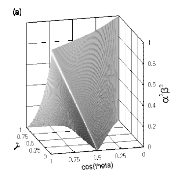
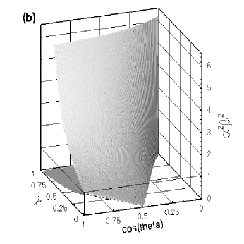
Figure 2: Surface of $\sigma=0.01$ for $E_{\omega}=0$. The horizontal plane is the $\gamma$-$\cos\theta$ plane and the vertical axis is $\alpha^{2}\beta^{2}$. Figure (a) shows the neutral surface for $0\leq\alpha^{2}\beta^{2}\leq 1$ and is an expansion of the boxed region in figure (b). For $\alpha=0$, the critical stability point occurs at $\theta=\pi/3$, which agrees with the classical results. The critical stability point shifts towards $\cos\theta=1$ as $\alpha^{2}\beta^{2}$ increases according to $\cos\theta=(1+\alpha^{2}\beta^{2})/2$. As $\alpha^{2}\beta^{2}$ exceeds unity, a stable band of rotating flows with nonzero eccentricities appears.

Thus, the LANS$-\alpha$ turbulence model enhances the growth rates of the elliptic instability for long waves with $\alpha^{2}\beta^{2}<1$ while it shifts the angle of critical stability along the cusp rising diagonally in Fig. 2. It also stabilizes the elliptic instability for short waves with $\alpha^{2}\beta^{2}>1$ as seen in Fig. 2b. Finally, for any $\alpha^{2}\beta^{2}\neq 0$, this turbulence model modifies the region in $(\gamma,\cos\theta)$ parameter space where the elliptic instability occurs, as also shown in Fig. 2.

In principle, one can now examine the stability properties of this new family of exact $\alpha-$CC solutions of the LANS$-\alpha$ model. This would be a secondary stability analysis of the rotating base flow. Work of this type was carried out by Lifschitz and collaborators lif:fab for the classical CC flows under high-frequency, short wavelength perturbations. A similar perturbation analysis for the $\alpha$-CC flow will be carried out elsewhere.

The authors are indebted to A. Lifschitz-Lipton for stimulating our original interest in CC solutions and to the Center for Scientific Computing at Southern Methodist University for use of their computing resources. Furthermore, BF thanks the Theoretical Division at the Los Alamos National Laboratory for their hospitality. The solutions to ${\mathbf{a}}(t)$ were simulated using the variable coefficient ODE solver DVODE dvode .

References

(1)
Lord Kelvin,
Phil. Mag. 24, 188 (1887).
(2)
A. Craik and W. Criminale,
Proc. R. Soc. London A 406, 13 (1986).
(3)
B. Bayly,
Phys. Rev. Lett. 57, 2160 (1986).
(4)
R. Kerswell,
Annu. Rev. Fluid Mech. 34, 83 (2002).
(5)
S. Chen, C. Foias, D. Holm, et al.,
Phys. Rev. Lett. 81, 5338 (1998);
Physica D 133, 49 (1999);
Phys. Fluids 11, 2343 (1999).
(6)
S. Chen, D. Holm, L. Margolin, and R. Zhang,
Physica D 133, 66 (1999).
(7)
D. Holm, J. Marsden, and T. Ratiu,
Adv. Math. 137, 1 (1998);
Phys. Rev. Lett. 80, 4173 (1998).
(8)
C. Foias, D. Holm, and E. Titi,
Physica D 152-153, 505 (2001).
(9)
J. Marsden and S. Shkoller,
Proc. Roy. Soc. London A 359, 1449 (2001);
C. Foias, D. Holm, and E. Titi,
J. Dyn. and Diff. Eqns. 14, 1 (2002);
D. Holm,
J. Fluid Mech. (to be published).
(10)
J. Dunn and R. Fosdick,
Arch. Ration. Mech. Anal. 56 191 (1974);
R. Larson,
Rheol. Acta 31, 213 (1992).
(11)
V. Yakubovich and V. Starzhinskii,
Linear Differential Equations with Periodic Coefficients,
Wiley, 1967.
(12)
F. Waleffe,
Phys. Fluids A 2, 76 (1990).
(13)
A. Lifschitz and B. Fabijonas,
Phys. Fluids 8, 2239 (1996);
B. Fabijonas, D. Holm, and A. Lifschitz,
Phys. Rev. Lett. 78, 1900 (1997);
A. Lifschitz, T. Miyazaki, and B. Fabijonas,
Eur. J. Mech. B/Fluids 17, 605 (1998);
B. Fabijonas and A. Lifschitz,
Z. Angew. Math. Mech. 78, 597 (1998).
(14)
P. Brown, G. Byrne, and A. Hindmarsh,
SIAM J. Sci. Stat. Comput. 10, 1038 (1989).