Using of Phenomenological Piecewise Continuous Map
for Modeling of Neurons Behaviour

Abstract

A piecewise continuous map for modeling bursting and spiking behaviour of isolated neuron is proposed. The map was created from phenomenological viewpoint. The map demonstrates oscillations, which are qualitatively similar to oscillations generating by Rose–Hindmarsh model. The synchronization in small ensembles of the maps is investigated. It is considered the different number of elements in the ensemble and different connectivity topologies.

]

I Introduction

Investigations of neuron ensembles (Central Pattern Generators, CPG) from the nonlinear dynamics viewpoint attract attention of many physicists last years. It is known some successful experiments with biological neurons (see, for example, [1]). Now exist a lot of mathematical models describing neuron behavior on the basis of ordinary differential equations [2]. Even simple models such as well-known FitzHugh–Nagumo and Rose–Hindmarsh systems, which may describe some important facts of neuron dynamics, need a lot of resources in numerical experiments for rather large ensembles. In this case the models with discrete time (maps) are much more appropriate.

It is known a set of such kind maps (i) the model with variable taking the discrete set of values (finite automata) [3, 4], (ii) the map taken on the flow of differential equations system [5], (iii) learning globally coupled excitable map system [6], (iv) recently proposed two-dimensional map [7]. However, the variety of models and methods for the neuron dynamics descriptions testifies that nonexists the common approach for creation of maps defining the isolated neuron behavior as well as for creation of the model neuron ensembles with pregiven topology and coupling kind.

In this paper is proposed a map with variable that changes continuously in specified range. This map demonstrates behavior that is qualitatively similar to the real neuron dynamics. It will be shown below that proposed map describes the complete synchronization in neuron ensembles. It will be also observed dependence the synchronization degree of the network configuration. Another results that will be discussed connected with the influence of external force on studied ensembles.

II The single neuron model

The map was constructed on the assumption of phenomenological conceptions. The basic idea is founded on the fact that in neuron behavior at time series the three regions (rest, burst and spike regions) could be identified. This relative division is schematically shown in Fig. 1.

The map ($x\rightarrow x^{\prime}$) consists of two piecewise continuous functions connected by transition conditions. The system dynamics is described with four state variables: $x\in[0,1]$, $d=\{-1,1\}$, $s_{1},s_{2}=\{0,1\}$. The main “observable” variable $x$ qualitatively corresponds to membrane potential of the neuron, the variable $d$ is used to select one of two branches of function and the variables $s_{1},s_{2}$ are “switches”, which define the conditions for burst ending. In mathematical notation the map are written in the following way.

FIG. 1.: The fragment of time series of isolated biological neuron (”1” is the rest state region, ”2” is the burst and ”3” is the spikes).

If $d=1$ (the increasing of the $x$ value)

$${x}^{\prime}={\left\{{\begin{array}[]{lll}\alpha_{1}\arctan(k_{1}x),&\mbox{if}&x\in\left[0,a-\delta_{1}\right),\\ 2a-x,&\mbox{if}&x\in\left[a-\delta_{1},a\right),\\ \gamma_{1}\left(x-a\right)+a,&\mbox{if}&x\in\left[a,c\right),\\ \end{array}}\right.}$$ (1)

The transition condition: $d=-1$ if $x\in[c,1]$.

If $d=-1$ (the decreasing of the $x$ value)

$${x}^{\prime}={\left\{{\begin{array}[]{lll}\frac{1}{\gamma_{2}}\left(x-a\right)+a,&\mbox{if}&x\in{\left[a+\delta_{2},1\right]},\\ 2a-x,&\mbox{if}&x\in\left[a,a+\delta_{2}\right),s_{1}s_{2}=1\\ \frac{1}{\alpha_{2}}\arctan(k_{2}x),&\mbox{if}&x\in\left[\delta_{3},a\right).\\ \end{array}}\right.}$$ (2)

Additional terms: $d=1$ if $x\in\left[a,a+\delta_{2}\right)$ and $s_{1}s_{2}=0$,

$\displaystyle s_{1}={\left\{{\begin{array}[]{lll}1,&\mbox{if}&x\in{\left[c,h_{1}\right]},\\ 0,&\mbox{if}&x\in{\left[0,a\right]},\\ \end{array}}\right.}\quad s_{2}={\left\{{\begin{array}[]{lll}1,&\mbox{if}&x\in{\left[{h_{2},1}\right]},\\ 0,&\mbox{if}&x\in{\left[{0,a}\right]},\\ \end{array}}\right.}$

$d=1$ if $x\in\left[0,\delta_{3}\right)$.

Here $a$, $k_{1}$, $k_{2}$, $\gamma_{1}$, $\gamma_{2}$, $\delta_{1}$, $\delta_{2}$, $\delta_{3}$ are some constant parameters, and others coefficients are determined from continuity condition ($c=(1-a)/\gamma_{1}+a,\alpha_{1}=a/\arctan(k_{1}a)$, $\alpha_{2}=a/\arctan(k_{2}a)$). Parameter $h_{2}$ is also constant and close to unity, and $h_{1}$ should depend on the value of $c$, that is $h_{1}=c+\Delta h$, where $\Delta h$ is the relatively small parameter.

FIG. 2.: The iteration diagram for the map, describing by (1), (2) transition conditions.

For better understanding how this map works the iteration diagram is shown in the Fig. 2. Fig. 3 demonstrates the time series for the isolated model neuron described by the map for various values of control parameters.

III Generalization of the model to coupled neurons. Two coupled neurons

Investigation of single neuron behavior has a little practical sense. Much more interesting might be model of neuron ensemble. Therefore this piecewise continuous map was generalized to coupled neuron systems. In case of the ensemble with $N$ elements with state variables $\left({x_{n}^{1},x_{n}^{2},...,x_{n}^{N}}\right)$ the influence of neighbours to $j$-th neuron at ($n+1$) discrete time is given by adding the following term to $x_{n+1}^{j}$ variable

$${\frac{{1}}{{L_{j}}}}{\sum\limits_{\begin{array}[]{l}{i=1}\\ {i\neq j}\\ \end{array}}^{N}{\varepsilon_{ij}\left({x_{n}^{i}-x_{n}^{j}}\right)\Theta\left({x_{n}^{i}-a}\right)}},$$ (3)

where $\varepsilon_{ij}$, ($i,j=1,...,N$) is the connection weight between $i$-th and $j$-th elements, $L_{j}$ is the number of neighbours of $j$-th neuron, $\Theta$ is the Heaviside step function (authors presume that exists a threshold of interaction).

The first investigated small ensemble was constructed of two coupled neurons. The main interest of the system research was consisted in revealing complete synchronization. The degree of synchronization was determined as

$$\Delta=\frac{1}{M}{\sum\limits_{n=1}^{M}{\left|x_{n}^{1}-x_{n}^{2}\right|}},$$ (4)

where $M$ is the number of iterations for a discrete time average.

FIG. 3.: Characteristic time series for isolated model neuron for $\delta_{2}=0.001$, $h_{1}=0.88$, $\gamma_{1}=1.4$, $\gamma_{2}=1.75$ (a); $\delta_{2}=0.001$, $h_{1}=0.88$, $\gamma_{1}=1.402$, $\gamma_{2}=1.75$ (b); $\delta_{2}=0.0001$, $h_{1}=0.92$, $\gamma_{1}=1.3$, $\gamma_{2}=1.3$ (c). The values of the other parameters are $a=0.3$, $k_{1}=0.9$, $k_{2}=1.0$, $h_{2}=0.95$, $\delta_{1}=0.01$, $\delta_{3}=0.001$.

Value $\Delta=0$ corresponds to the highest degree of synchronization, $\Delta>0$ means that the synchronization is absent or synchronization is incomplete. In this research the degree of synchronization (4) on the plane of parameters $\left(\varepsilon,\gamma_{1}\right)$ is calculated. The choice of parameter $\varepsilon$ as a control parameter is natural because it’s value determines the strength of connection. The value of parameter $\gamma_{1}$ (as well as $\gamma_{2}$) influences considerably to the system behavior, so it is chosen as second control parameter. The parameter planes are plotted in grayscale, namely, synchronization (for value $\Delta=0$) region marked with the white color, the positive value of $\Delta$ is subjected to the simple rule: the larger value, the darker point. Such parameter plane for two coupled neurons is presented in Fig. 4. The behavior of this system in some points, marked on the parameter plane with letters, is shown in Fig. 5.

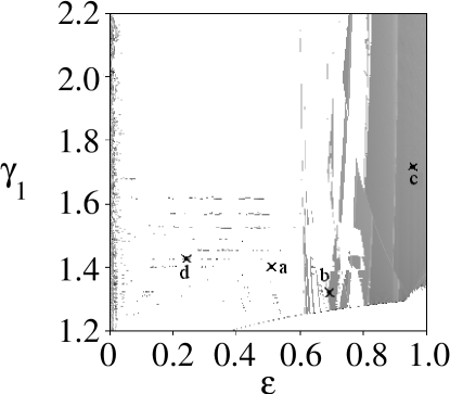
FIG. 4.: The parameter plane, plotted for two coupled model neurons. The letters correspond to time series, presented in Fig. 5. The values of the other parameters are $a=0.3$, $k_{1}=0.9$, $k_{2}=1.0$, $\gamma_{2}=1.75$, $\delta_{1}=0.01$, $\delta_{2}=0.001$, $\delta_{3}=0.001$, $h_{2}=0.95$.

It was revealed that the system dynamics depends on the initial conditions therefore the question about typicalness of presented parameter plane occurs. This problem was studied in detail. The view of the attraction basins, plotted in different points of the parameter plane, and the parameter planes obtained for various initial conditions shows that the general features of the planes are invariable, so this question will be not discussed below.

IV Systems with several elements

In the research is observed a large quantity of neuron ensembles with different numbers of elements and various spatial configurations. Some revealed regularities for ensemble of seven coupled neurons is presented here.

In case of several elements the degree of synchronization can’t be defined with (4), therefore in numerical experiments is used the following approximate relationship

$\displaystyle\Delta=\frac{1}{M}{\sum\limits_{n=1}^{M}\left|{x_{n}^{k}-\frac{1}{N}{\sum\limits_{i=1}^{N}{x_{n}^{i}}}}\right|}.$

FIG. 5.: Characteristic time series plotted for two coupled neurons in the points, marked on the parameter plane in fig. 4 with $\varepsilon=0.50$, $\gamma_{1}=1.40$ (complete synchronization) (a); $\varepsilon=0.95$, $\gamma_{1}=1.70$ (b); $\varepsilon=0.24$, $\gamma_{1}=1.427$ (c).

Fig. 6 presents the parameter planes that are gotten for systems schematically shown at the insets. As it can be seen, the areas with synchronous behaviour become larger when additional connections are inserted. Note, that although this tendency is clearly visible from Fig. 6, the synchronous behaviour is observed in another areas of the parameter plane (see Fig. 6b and Fig. 6c). Comperison of Fig. 6b and Fig. 6c shows that synchronization degree is decreased in the region $\varepsilon\in[0.8;~{}1.0]$ for all values $\gamma_{1}$. This result remains correct for systems with another numbers of elements.

It was shown that the synchronization degree depends on the fast motion (the spikes region) and practically is independent of slow motions. This fact was revealed when the nonlinear branches (see Fig. 2, region $x_{n}\in[0;~{}a]$) of the map functions (1), (2) were approximated with piecewise linear functions. There is the visible changes of the time series, but the view of parameter planes remains without any considerable changes.

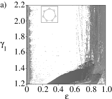
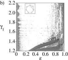
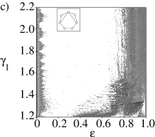
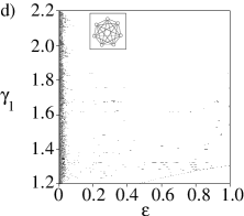
FIG. 6.: The planes of parameter for ensembles with seven elements and different spatial configurations (shown at the insets) obtained from ring-type system by adding of connections.

V The influence of the external action

The investigations of the synchronization also involved the possibility to influence on this process with an external signal. It was revealed that an external low-amplitude spatially uniform field (both periodical and chaotic) may increase the degree of synchronization in the ensemble. As the example of this fact the parameter planes are presented for ring-type system with seven neurons under an external force (Fig. 7).

As one can see from comparison of the parameter plane in Fig. 7 and Fig. 6a, the region of synchronous behaviour for the model neuron ensemble under the external force becames larger in relation to the region for unperturbated system.

VI Conclusion

In this work the phenomenological map describing some aspects of neuron dynamics is presented. It is shown that the proposed map qualitatively simulates real neuron behavior and describes some synchronization phenomena that is observed in neuron ensembles, connected via electrical synapse. The assumption that just fast motion is responsible for the synchronization phenomena is prior and should be confirmed. The results related to a possibility of low-amplitude external field to increase the degree of synchronization in small model neuron ensemble may be useful from the practical viewpoint but only in case that they will get an experimental verification.

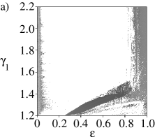
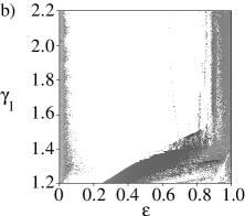
FIG. 7.: The ring-type system with seven elements under the low-amplitude spatially uniform periodic (a) and chaotic (b) fields $\xi_{n}=ay_{n}$, where $a=0.0003$. The periodic field is generated by $y_{n}=\sin\left(2\pi n/T\right)$ with $T=500$ and chaotic one by the logistic map $y_{n+1}=1-\lambda y_{n}^{2}$ with parameter $\lambda=1.99$.

The way on the creation of the piecewise map from phenomenological viewpoint (from view of the system time series), applied in the work, could be used for other sysnems.

This work was supported by RFBR under grants 02-02-16351, 00-15-96673, Program ”Universities of Russia” and Ministry of Education of Russian Federation under grant E00-3.5-196.

REFERENCES

- [1] R.C. Elson, A.I. Selverston, R. Huerta, N.F. Rulkov, M.I. Rabinovich, and H.D.I. Abarbanel, Phys. Rev. Lett. 81 (25), 5692–5695 (1998).
- [2] H.D.I. Abarbanel, M.I. Rabinovich, A.I. Selverston, M.V. Bazhenov, R. Huerta, and M.M. Sushchik, Phys. Usp. 39 (4), 337–362 (1996).
- [3] M.I. Rabinovich, A.I. Selverston, L. Rubchinsky, and R. Huerta, Chaos 6 (3), 288–296 (1996).
- [4] R. Huerta, Int. J of Bifurcation and Chaos 6 (4), 705–714 (1996).
- [5] I.V. Belykh, Izvestya VUZ Radiofizika 41 (12), 1572–1580 (1998). (in Russian).
- [6] Y. Hayakawa, and Y. Sawada, Phys. Rev. E 61 (5), 5091–5097 (2000).
- [7] N.F. Rulkov, Phys. Rev. Lett. 86 (1), 183–186 (2001).