Homogeneous isotropic turbulence in dilute polymers: scale by scale budget
E. De Angelis , C.M. Casciola^∗, R. Benzi , & R. Piva^∗

Abstract

The turbulent energy cascade in dilute polymers solution is addressed here by considering a direct numerical simulation of homogeneous isotropic turbulence of a FENE-P fluid in a triply periodic box. On the basis of the DNS data, a scale by scale analysis is provided by using the proper extension to visco-elastic fluids of the Karman-Howarth equation for the velocity. For the microstructure, an equation, analogous to the Yaglom equation for scalars, is proposed for the free-energy density associated to the elastic behavior of the material. Two mechanisms of energy removal from the scale of the forcing are identified, namely the classical non-linear transfer term of the standard Navier-Stokes equations and the coupling between macroscopic velocity and microstructure. The latter, on average, drains kinetic energy to feed the dynamics of the microstructure. The cross-over scale between the two corresponding energy fluxes is identified, with the flux associated with the microstructure dominating at small separations to become sub-leading above the cross-over scale, which is the equivalent of the elastic limit scale defined by De Gennes-Tabor on the basis of phenomenological assumptions.

I Introduction

Turbulence in dilute polymers solutions is still an open issue, despite the growing interest on the subject. Most of the efforts have been addressed to the comprehension of practical aspects, such as drag reduction, related to the modification of turbulence by long chain polymers in wall bounded flows, [17]. However, in most cases, the attempts have proven inconclusive, suggesting that, even from the point of view of applications, a more fundamental approach is required. Under this respect, basic studies should focus on simpler flow conditions where turbulence-polymers interaction occurs.

A possible choice is to exploit homogeneity and isotropy to simplify the statistical treatment of the data and to make use of the available, relatively well established, rheological models for dilute polymers, see [2] for a comprehensive review.

In this context, a recent experimental investigation on decaying grid turbulence of dilute polymers and surfactants [10] shows, for the polymers, a substantial alteration of the small scales, though still in presence of a substantial degree of anisotropy, ascribed to the grid shear layers.

In this and other related experiments, see e.g. [20] and [11], the measurements were mostly aimed at the velocity, but also at the pressure field see e.g. [3] for a recent example. Actually, as one can imagine, the experimental analysis of turbulent flows of polymeric liquids is particularly difficult, and hardly one can proceed beyond the global characterization of the flow and the analysis of certain aspects of the macroscopic field, see [16], [26] as additional examples in the more complex configuration of a channel flow. This makes the actual mechanism of interaction between polymers and turbulence particularly obscure, and leads to consider numerical simulations as a viable tool to address the problem. For triply-periodic boundary conditions, in particular, fast and accurate spectral methods can easily be developed to achieve the direct numerical simulation of a strictly homogeneous isotropic flow, once a reasonably accurate and sufficiently simple rheological model has been selected. Among these, the so-called FENE-P model [25] is possibly the best compromise between accurate representation of polymers dynamics and minimal computational complexity, see [15]. In fact, recent results show that this model is able to reproduce the drag reducing behavior of dilute polymers in wall bounded flows, see [24], [6], [7].

As often in rheology, one can easily get stuck in a discussion about the proper model for a specific application. We take here the model for granted and try to grasp the mechanisms by which it affects the turbulence. To do this we take freedom to chose parameter values which may not correspond too well to experimental conditions, but which may help revealing the underlying physics.

In summary, our model for the solution considers an ensemble of elastic dumbbells attached to each material point of the continuum. The dumbbells are stretched by the flow due to friction and react through a non-linear elastic spring. The probability density function of the end-to-end vector of the dumbbells is described through a second order tensor, the conformation tensor, assumed to represent the covariance matrix of the end-to-end vectors. It obeys a transport equation which accounts for material stretching and for the elastic reaction. The force exerted on the continuum by the dumbells contributes an extra-stress term in the macroscopic momentum balance. On average, the work done by the extra-stress against the macroscopic velocity field amounts to a draining of energy from the macroscopic field. The corresponding power feeds the dynamics of the microstructure, is partially accumulated as free-energy of the ensemble and is eventually dissipated, see [8].

In terms of turbulence dynamics, several basic questions arise. First of all, one should understand if the nature of this kind of viscoelastic turbulence is substantially similar, or, on the contrary, essentially different from standard Newtonian turbulence. According to the common view, a turbulent flow is described as a superposition of different scales of motion. In homogeneous isotropic turbulence of ordinary fluids the interaction of the different scales originates a flux of energy from the large towards the small scale, with energy injected by an external forcing at large scales and dissipated by viscosity at small scales, the so-called direct, or forward, energy cascade (see e.g. the book by Frisch [12]). The presence of the microstructure is expected to alter this process, since it corresponds to an alternative path the energy flux may take to achieve the eventual dissipation. If this is the case, one may wonder if the alteration is localized at certain spatial scales or if the entire spectrum is affected by the energy draining of the polymers. This poses the additional issue of determining a possible scale which delimits the range of scales where the presence of the polymers is effective from those where they are substantially passive, see [9]. This scale may be close to the classical Kolmogorov dissipation scale, but it may even be substantially larger, and it is not even clear if the effect of polymers may be reduced to an additional dissipation, [18], or if the role of elastic energy is crucial, [9], see also [23].

All these issues can be addressed systematically by analyzing the data of a DNS of homogeneous isotropic turbulence once proper diagnostic tools are available. To this purpose we present and discuss a scale by scale budget based on the extension to viscoelastic fluids of the classical Karman-Howarth [12] equation of ordinary turbulence, see e.g. [14], [22] and [4] for similar extensions in the context of shear flows. By this equation we can address the effect of polymers on the macroscopic kinetic field. To consider the fluctuations in the polymers we would need to extend the classical Yaglom equation for a scalar, see [21], to a second order active tensor. In a more straightforward way instead we consider, in the proper thermodynamic framework, the Yaglom equation for the free-energy of the polymers.

II The evolution equations for dilute polymer solutions

As discussed in the introduction, the momentum balance for a dilute solution of long chain polymers in otherwise Newtonian, incompressible solvent is described by a slightly modified form of the Navier-Stokes equation, namely

$$\frac{Du_{i}}{Dt} = \frac{\partial p}{\partial x_{i}}\,+\nu\,\frac{\partial^{2}u_{i}}{\partial x_{j}\partial x_{j}}\,+\,\frac{\partial T_{ij}}{\partial x_{j}}\,+f_{i}\,,$$ (1)

where $D/Dt=\partial/\partial t\,+\,u_{k}\,\partial/\partial x_{k}$ is the usual substantial derivative, $f_{i}$ the external forcing, $p$ is the pressure normalized by the constant density of the solution, $\nu$ is the kinematic viscosity of the solvent and $T_{ij}$ is the additional contribution to the stress tensor - extra-stress - due to the polymers chains. The macroscopic velocity field $u_{i}$ is solenoidal and the constitutive relation for the extra-stress is

$$T_{ij} = \nu_{p}/\tau\,(\,f(R_{kk};\rho_{m},\rho_{0})R_{ij}/\rho_{0}^{2}-\delta_{ij}\,)\,,$$ (2)

where $\nu_{p}$ is a constant typically of the order of a small but finite fraction of $\nu$. The conformation tensor, $R_{ij}$, is a second order tensor taken to characterize the statistical behavior of the population of polymers chains attached to a given point, and $f(R_{kk};\rho_{m},\rho_{0})$ is a dimensionless nonlinear spring coefficient specified as $f=(\rho_{m}^{2}-\rho_{0}^{2})/(\rho_{m}^{2}-R_{kk})$, with $\rho_{0}$ the equilibrium length of the chains and $\rho_{m}$ their maximum allowed length, as standard in the context of the finite extensibility nonlinear elastic model (FENE, see [2]). The dynamics of the population of chains is described by an evolution equation for the conformation tensor,

$$\frac{DR_{ij}}{Dt} = \frac{\partial u_{i}}{\partial x_{k}}R_{kj}\,+\,R_{ik}\frac{\partial u_{k}}{\partial x_{j}}\,-\frac{1}{\tau}(fR_{ij}-\rho_{0}^{2}\delta_{ij})\,,$$ (3)

where $\tau$ is the principal relaxation time of the chains. The system (1, 2, 3) completed with the continuity equation,

$$\frac{\partial u_{i}}{\partial x_{i}} = 0\,,$$ (4)

for the macroscopic velocity forms the FENE-P model for dilute polymers solutions, see e.g. [25].

Phenomenologically, stretching of the chains by the flow, described by the terms involving the velocity gradient in (3), is counteracted by an elastic reaction, the term in brackets, while the polymers are transported and re-oriented by the flow. The reaction of the polymers alters the macroscopic force balance, as seen in eq. (1), where the divergence of the extra-stress enters as an additional source or sink of momentum.

The extra-stress is able to make work against the velocity as follows from the balance of kinetic energy

$$\frac{D(u^{2}/2)}{Dt}=\frac{\partial\,(p\,\delta_{ij}+\Sigma_{ij})\,u_{i}}{\partial x_{j}}\,+\,\frac{\partial\,(T_{ij}\,u_{i})}{\partial x_{j}}-\,\epsilon_{N}+\,S\,,$$ (5)

where $\Sigma_{ij}=2\nu e_{ij}$ is the standard viscous component of the stress tensor and $\epsilon_{N}=2\nu e_{ij}e_{ij}$ is the Newtonian component of the dissipation, with $e_{ij}$ the macroscopic velocity deformation tensor. With respect to the kinetic energy balance of the standard Navier-Stokes equation, two additional terms arise here, to describe the interaction of the macroscopic field with the microstructure. The one in divergence form contributes to the spatial redistribution of kinetic energy. The other,

$$S=T_{ij}\frac{\partial u_{i}}{\partial x_{j}}\,,$$ (6)

called hereafter the stress-power, represent energy per unit time that the microstructure can drain, or, in principle, even release to the macroscopic kinetic field. The presence of this term is physically due to the fact that the polymers chains can both dissipate, via friction with the solvent, or store energy, due to their elasticity. The correct thermodynamical setting refers to the free-energy $a$ of the polymers ensemble. Given the expression, see e.g. [2],

$$a=-\frac{1}{2}\frac{\nu_{p}}{\tau}\left[(\rho^{2}_{max}/\rho_{0}^{2}-1)\log\left(\frac{\rho^{2}_{max}-{R}_{kk}}{{\rho^{2}_{max}-\rho_{0}^{2}}}\right)\right.$$ (7)

(8)

$$\left.\qquad\qquad+1/3\,\log(\det{R/\rho_{0}^{2}})\right]\,,$$ (9)

it follows directly from the evolution equation (3) that the energy balance for the polymers is

$$\frac{Da}{Dt} = S-\epsilon_{P}\,,$$ (10)

where

$$\epsilon_{P}=\frac{1}{2}\frac{\nu_{p}}{\tau^{2}}f\,\left[(f\,R)_{kk}+(f\,R)^{-1}_{kk}-6\right]$$ (11)

a positive definite quantity, is the rate of energy dissipation associated with the polymers. Adding eq. (5) and (10) gives the balance of the total free-energy of the system, $E=u^{2}/2+a$, as

$$\frac{DE}{Dt} = f_{i}u_{i}-\epsilon_{T}+\frac{\partial J_{k}}{\partial x_{k}}$$ (12)

where $J_{i}$ is the spatial flux of total free-energy, whose expression follows immediately by inspection of the kinetic energy balance. Note that $S$ drops from the global balance since it corresponds to a conservative exchange of energy between the two constituents, namely the macroscopic kinetic energy and the polymers free-energy.

III The Karman-Howarth equation

In a statistically stationary turbulent system, the external forcing $f_{i}$ provides the energy to maintain the turbulent fluctuations which otherwise would be damped by the dissipation. For the present case both the macroscopic velocity and the microstructure exhibits turbulent fluctuations. Characteristic feature of the system is that, while the external forcing acts only on the macroscopic field, both the macroscopic flow and the microstructure contribute to the dissipation of the injected mechanical power. This is possible since the extra-stress captures part of the available mechanical energy to feed the fluctuations of the microstructure and the associated dissipation. In order to try to disentangle these complex processes, the simplest setting is provided by homogeneous and isotropic turbulence once suitable balance equation are available for the fluctuations of both kinds.

Purpose of the present section is to present the equation appropriate to address the scale by scale budget of the macroscopic velocity fluctuations. This is the extention to dilute polymer solutions of the well known Karman-Howarth equation of homogeneous isotropic turbulence for Newtonian fluids. As discussed in the previous section, where the FENE-P model has been briefly recalled, the solenoidal velocity field, $u_{i}$, obeys a modified form of the Navier-Stokes equation, where the divergence of the extra-stress $T$, denoted here by

$$g_{i} = \frac{\partial T_{ij}}{\partial x_{j}}\,,$$ (13)

appears as an additional source of momentum.

Starting with the modified Navier-Stokes equation, the equation for the correlation tensor $C_{i,j}=<u_{i}\,u^{\prime}_{j}>$, where unprimed and primed variables are evaluated at $x_{i}$ and at $x^{\prime}_{i}$, respectively, with $x^{\prime}_{i}$ the displacement of $x_{i}$ by the separation vector $r_{i}$, easily follows from the standard procedure, see e.g. [14], [21]. The trace of this equation reads

$$\frac{\partial C_{i,i}}{\partial t}+\frac{\partial}{\partial r_{k}}<u_{i}u^{\prime}_{i}u^{\prime}_{k}-u_{i}u^{\prime}_{i}u_{k}>=\qquad\qquad$$ (14)

$$2\nu\frac{\partial^{2}C_{i,i}}{\partial r_{k}\partial r_{k}}\,+\,<g^{\prime}_{i}u_{i}+g_{i}u^{\prime}_{i}>\,+\,<f^{\prime}_{i}u_{i}+f_{i}u^{\prime}_{i}>\,,$$ (15)

where $f_{i}$ is here specified as a random stirring force acting on the large scales. To obtain the above equation we have used standard properties of homogeneous incompressible turbulence, which allow to drop the pressure term and to recast spatial derivatives with derivatives with respect to the separation, see e.g. [12].

Equation (14) can be re-expressed in terms of velocity increments, $\displaystyle\delta V_{i}=u_{i}(x^{\prime}_{r})-u_{i}(x_{r})$, $\;\delta V^{2}=\delta V_{i}\delta V_{i}$, once recalled that $C_{i,i}=<u_{i}u_{i}>-1/2<\delta V^{2}>$, and that, by standard manipulations, we have

$$<\delta V^{2}\delta V_{k}>=-2<u_{i}u^{\prime}_{i}u^{\prime}_{k}-u_{i}u^{\prime}_{i}u_{k}>+$$ (17)

$$\qquad\qquad\qquad\qquad<u_{i}u_{i}u^{\prime}_{k}>-<u^{\prime}_{i}u^{\prime}_{i}u_{k}>\,.$$ (18)

Hence, for a solenoidal velocity field, the equation in terms of velocity increments follows as

$$\frac{\partial}{\partial r_{k}}<\delta V^{2}\delta V_{k}+2T^{*}_{ki}\delta V_{i}>=-4<f_{i}u_{i}>\,+\,$$ (19)

$$2<\delta V_{i}\delta f_{i}>\,+\,2\nu\frac{\partial^{2}}{\partial r_{k}\partial r_{k}}<\delta V^{2}>.$$ (20)

In deriving eq. (19) a statistically stationary field has been assumed and the term $<f^{\prime}_{i}u_{i}+f_{i}u^{\prime}_{i}>$ has been rearranged in the form $2<f_{i}u_{i}>-<\delta V_{i}\delta f_{i}>$ to extract explicitly the power injected by the external forcing. Finally, the integration by parts

$$<g^{\prime}_{i}u_{i}+g_{i}u^{\prime}_{i}>=\frac{\partial}{\partial r_{k}}(T^{\prime}_{ki}u_{i}-T_{ki}u^{\prime}_{i})=-\frac{\partial}{\partial r_{k}}(T^{*}_{ki}\delta u_{i})\,,$$ (22)

where $T^{*}_{ki}=T^{\prime}_{ki}+T_{ki}$, leads to eq. (19).

Equation (19) can be integrated in $r$-space over a ball $B_{r}$ of radius $r$ (see e.g. [4] for a similar approach) to yield

$$\frac{1}{4\pi r^{2}}\oint_{\partial B_{r}}<\delta V^{2}\delta V_{k}+2\,T^{*}_{ki}\,\delta V_{i}>n_{k}\,dS_{r}=-4/3\,\bar{\epsilon}_{T}\,r$$ (24)

$$+\frac{\nu}{2\pi r^{2}}\,\frac{d}{dr}\,\oint_{\partial B_{r}}<\delta V^{2}>\quad dS_{r}\,$$ (25)

$$+\frac{1}{2\pi r^{2}}\int_{B_{r}}<\delta V_{i}\delta f_{i}>\quad dV_{r}\,,$$ (26)

where the global energy balance (12), which for a stationary homogeneous field reads

$$<f_{i}u_{i}> = {\bar{\epsilon}}_{T}\,,$$ (28)

has been accounted for.

The Karman-Howarth equation (24) highlights the main difference between Newtonian and viscoelastic turbulence. For either case, in the range of scales where the direct effect of viscosity and the correlation between velocity and forcing increments are both negligible, the energy flux occurring through scale $r$ equals the total dissipation. For Newtonian fluids, all the dissipation is provided by the viscosity and the flux through scale $r$ only occurs due to the classical nonlinearity associated to the advection. For viscoelastic fluids, an additional dissipative process takes place in the polymers, and, consistently, the flux through scale $r$ also presents a new component in addition to that of the standard Navier-Stokes dynamics. In fact, the additional flux term describes the amount of energy intercepted by the microstructure. Though the classic component is expected to be associated to a forward energy cascade, i.e. the corresponding flux enters the ball of radius $r$, concerning the viscoelastic contribution we can, at the moment, only conjecture that energy intercepted at scale $r$ is passed forward to the microstructure at smaller scale, consistently with the idea of polymer dissipation as a small scale process. However, since, to our knowledge, the process has never been investigated before, we have to examine and discuss the numerical simulation before drawing any conclusion.

IV The Yaglom equation for the free-energy

The Karman-Howarth equation for dilute polymer solution may be used to analyze the scale by scale budget for the velocity field. Its Fourier transform actually corresponds to the budget of turbulent kinetic energy in the different modes of the spectrum. To address the complete dynamics of dilute polymers solution we need a similar equation concerning the microstructure. Under this respect, in section 1 we have shown that a free-energy $a$ can be associated to the ensemble of polymers attached to a given point in space and that, locally, the energy balance for the microstructure is provided by equation (10).

The free-energy $a$ is a measure of the average elongation of the polymers as given by the trace of the conformation tensor $R_{ij}$. In fact one can derive an equation for the scale by scale budget of the trace though we prefer to discuss the Yaglom equation for $a$, whose meaning in terms of energetics of the system is more definite. To this purpose, let us denote by

$$\psi=S-\epsilon_{p}$$ (29)

the instantaneous excess power, i.e. the amount of power transfered to the polymers in excess to the dissipation they originate. Strictly speaking this is an improper naming, since on the average the excess power is zero. Nonetheless, it measures the amount of energy stored per unit time in the polymers. From (10) we can derive the equation for the correlation $<aa^{\prime}>$,

$$\frac{\partial<aa^{\prime}>}{\partial t}\,+\,\frac{\partial}{\partial r_{k}}<u^{\prime}_{k}a^{\prime}a-u_{k}aa^{\prime}> =$$ (30)

$$<a^{\prime}\psi+a\psi^{\prime}>\,,$$ (31)

which, considering that

$\displaystyle<a\psi^{\prime}+a^{\prime}\psi>=2<a\psi>-<\delta a\delta\psi>\,,$

and noting that, for a stationary state ($<a\,{Da}/{Dt}>=0$),

$$<a\psi>=0\,,$$ (32)

can be recast in the form

$$\frac{\partial}{\partial r_{k}}<\delta u_{k}\delta a^{2}>=2<\delta a\delta\psi>\,.$$ (33)

Integration over the sphere of radius $r$ then yields

$$\frac{1}{4\pi r^{2}}\oint_{\partial B_{r}}<\delta a^{2}\delta V_{k}>n_{k}dS_{r} =$$ (34)

$$\frac{2}{4\pi r^{2}}\int_{B_{r}}<\delta a\delta\psi>dV_{r}\,,$$ (35)

which, by using isotropy reduces to

$$<\delta a^{2}\delta V_{\parallel}> = 2\int_{0}^{r}<\delta a\delta\psi>r^{2}dr\,,$$ (36)

with $\delta V_{\parallel}=\delta V_{i}\,r_{i}/r$ the longitudinal velocity increment.

Equation (36) is the appropriate form of the Yaglom equation for the polymers. It states the equivalence between the flux of free energy through the different spatial scales, as described by $<\delta a^{2}\delta V_{\parallel}>$ and the integral of the correlation between free energy fluctuations, $\delta a$, and fluctuation of the excess of power, $\delta\psi$. Classically for scalars the Yaglom equation provides a term linear in the separation associated to the average scalar dissipation. In the present case, such term is zero as consequence of eq. (32).

V Global features of the flow and DNS

The system of equations (1,3,4), corresponding to $9$ scalar equation, $3$ velocity components plus $6$ components of the conformation tensor, has been integrated using a Fourier $\times$ Fourier $\times$ Fourier spectral method for spatial discretization and a four-stages/third order Runge-Kutta method for time advancement with all the non-linear terms fully de-aliased by the three-halves rule. An exactly solenoidal velocity is achieved by the standard projection method. The side of the cubic computational box is $2\pi$ and $64$ modes are used in each direction. A fully developed field of Newtonian turbulence has been used as initial condition for the viscoelastic calculation and the random forcing is applied to the first shell of wave-vectors, with constant amplitude and uniformly distributed phases. The random phase extracted at each step is used subject to the condition of positive energy injection, otherwise it is changed by $\pi$.

The nominal Reynolds number of the simulation can be constructed from the intensity of the forcing, $\hat{f}_{0}$, the length of the box, $l_{x}$, and the zero shear kinematic viscosity, $\nu_{T}=\nu+\nu_{P}$, as $Re=(l_{x}^{3}\hat{f}_{0})^{(1/2)}/\nu_{T}=676$. The parameters concerning the polymers are $\eta_{p}=\nu_{p}/\nu=.1$, see e.g. [10], $\rho^{2}_{m}/\rho^{2}_{0}=1000$ and $De=\tau(\hat{f}_{0}/l_{x})^{1/2}=.38$. When comparing viscoelastic and Newtonian simulations, we keep constant the nominal Reynolds number, i.e. for the Newtonian case we use the same forcing intensity and a value for the viscosity equal to the value of $\nu_{T}$ for the viscoelastic fluid.

After the transient is elapsed, statistically stationary conditions are achieved. The general impression on the field may be gained by considering figure 1, where instantaneous vortical structures are shown for the Newtonian and the viscoelastic simulation. The eduction criterion for vortical structures is based on the discriminant of the velocity gradient tensor, one of the now classical approaches to extract vortical structures from a complex field, see e.g. [5] for details. Algebraically, the idea is to identify with vortical structures those regions where a couple of eigenvalues of the velocity gradient are complex conjugate, implying a locally helicoidal relative motion of nearby particles. In principle, other criteria could be employed and different field quantities could be visualized. In any case, the inspection of the instantaneous fields always leads to the conclusion that, with respect to Newtonian, much less but wider structures are present in the viscoelastic case.

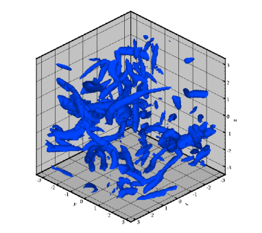
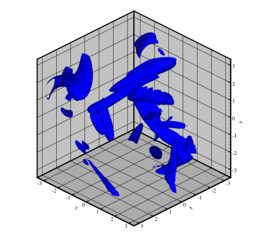
FIG. 1.: Vortical structures for the Newtonian, $De=0$, (top) and viscoelastic case, $De=.38$, (bottom).

Table I presents the global parameters of a typical viscoelastic simulation, $De=.38$, together with a corresponding Newtonian case. In the table, the Taylor microscale is defined as $\lambda=(15/2\,u_{rms}^{2}/\Omega)^{1/2}$, with $\Omega=1/2<\zeta^{2}>$, $\zeta$ being the vorticity. The average value of the free-energy is denoted by $\bar{a}$, while the other symbols have been already defined in the previous sections. Concerning the Kolmogorov scale, $\eta$, for the viscoelastic case this quantity is not uniquely defined. Actually, for Newtonian turbulence one assumes that the small scale dynamics is controlled by dissipation and viscosity, originating the classical definition of the Kolmogorov length as $\eta=(\nu^{3}/\epsilon)^{1/4}$. In the present case, several other parameters related to the more complex rheology may in principle affect the small scale dynamics. In the table we have conventionally assumed $\eta_{T}=(\nu_{T}^{3}/\epsilon_{T})^{1/4}$.

$De$	$Re_{\lambda}$	$u_{rms}$	$\Omega$	$\bar{a}$	$\bar{\epsilon}_{T}$	$\bar{\epsilon}_{N}$	$\bar{\epsilon}_{P}$	$\lambda$	$\eta_{T}$
0	75	.806	10.6	-	.156	.156	-	.68	.040
.38	170	.9685	5.1	.09	.231	.067	.164	1.18	.036

TABLE I.: Global parameters for the Newtonian, $De=0$, and the viscoelastic, $De=.38$, simulation.

By discussing the data in table I, the macroscopic effects of viscoelasticity can be summarized as follows. For fixed forcing amplitude, i.e. for fixed nominal Reynolds number in identical boxes and with same total viscosity, $\nu_{T}$, we observe a substantial increase of the total dissipation. Clearly, in the steady state, this corresponds to an equivalent increase in the power extracted from the external forcing. For the viscoelastic case, most of the dissipation, about $71\%$, occurs in the polymers. The $u_{rms}$ increases of about $20\%$, with respect to the Newtonian simulation. The increase of the energy content in the flow is even more apparent if we consider that, in addition to kinetic energy, a non-negligible contribution arises from the free energy $\bar{a}$. In terms of total energy, $\bar{E}=3/2\,u^{2}_{rms}+\bar{a}$, the increase with respect to Newtonian turbulence is of the order of $48\%$. Clearly, the increase in the total dissipation for fixed total viscosity amounts to a reduction of the conventional Kolmogorov scale.

A further effect is observed when comparing the Taylor microscale for the two simulations. The increase in turbulent kinetic energy of about $44\%$ is accompanied by

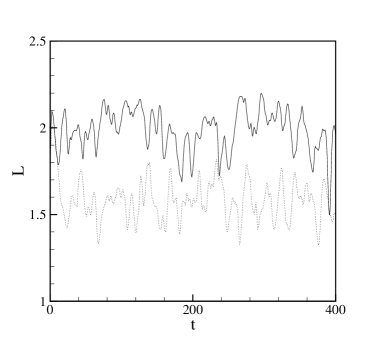
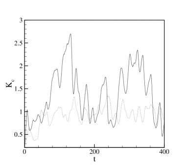
FIG. 2.: Top: Time behavior of the integral scale for the Newtonian, (dotted) and viscoelastic, (solid) case. Bottom: Time behavior of the spatial average of the turbulent kinetic energy, same symbols.

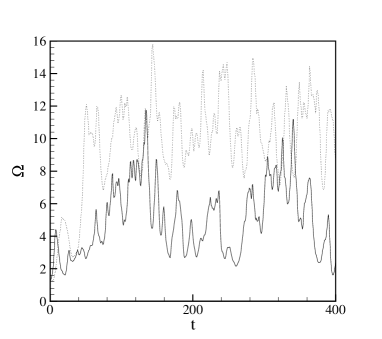
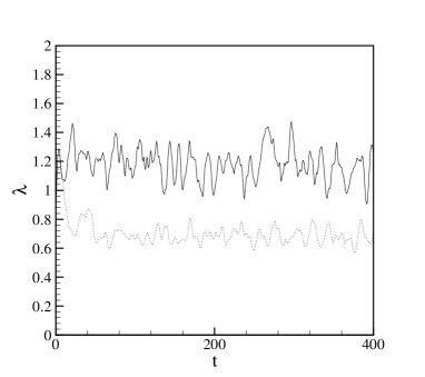
FIG. 3.: Top: Time behavior of the spatial average of the enstrophy for the Newtonian, (dotted), and the viscoelastic case, (solid). Bottom: Time behavior of the Taylor microscale, same symbols.

a reduction of the order of $50\%$ in the enstrophy, giving an increase of $73\%$ for the Taylor microscale. This suggests a substantial depletion in the energy content of the high wave-number modes. Consistently a substantial increase in the Taylor-Reynolds number, $Re_{\lambda}=u_{rms}\lambda/\nu_{T}$, is achieved.

From the numerical point of view, a comparable value for $Re_{\lambda}$ in Newtonian fluids cannot be reached with only $64$ spatial modes. For the viscoelastic case, however, the requirements on the grid are less strict, since most of the dissipation, the polymeric contribution, is not associated to spatial gradients. We observe in passing, that spectral calculation with the FENE-P model may be prone to high-wavenumber instability, which is maintained under control by adding a small amount of artificial viscosity in the algorithm for the conformation tensor [24], see also [19] for an alternative approach.

The evolution of the system, followed for about $50$ large-eddy turnover times, $T=(l_{x}/\hat{f}_{0})^{1/2}=7.9$, is globally described in figure 2, where the time history of the instantaneous integral scale $L=\pi/2\int_{0}^{K_{max}}1/k\,{\hat{e}}(k)\,dk\,/\,u^{2}_{rms}$, where $\hat{e}$ is the instantaneous energy spectrum, is shown on the top. From the comparison between viscoelastic and Newtonian case, the average increase in $L$ is apparent. Clearly this is associated to the increase in the amount of energy in the energy containing range, and corresponds to the observation of larger structures in the field. The presence of fewer but more energetic coherent structures is also consistent with the existence of more pronounced intermittency cycles, more evident in the history of the kinetic energy shown on the bottom part of the same figure.

Figure 3 describes the evolution of enstrophy, top, and Taylor microscale, bottom. On average, the enstrophy reduces with respect to Newtonian turbulence, and presents large spikes following with slight delay the corresponding peaks found in the kinetic energy. In figure 4 we report on top the time behavior of the spatial average of the free energy. Apparently, the amount of energy stored by the polymers is substantially lower than the kinetic energy, already given in figure 2 and reproduced

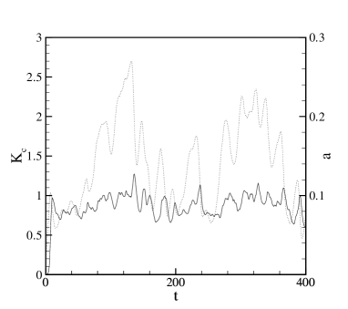
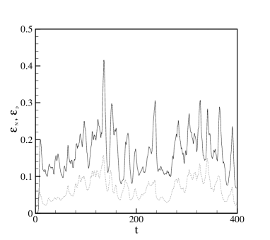
FIG. 4.: Viscoelastic simulation, $De=.38$. Top: Time behavior of the spatial average of the free-energy, $a$, (solid) compared with the kinetic energy (dotted). Note the scales, differing by an order of magnitude, for free-energy on the right and kinetic energy on the left. Bottom: Time behavior of the spatial average of the Newtonian (dotted) and the viscoelastic component (solid) of the dissipation.

here for convenience. From the comparison one may note the more irregular behavior of the free-energy with reduced peak to peak oscillations. Finally, on the bottom of the figure we plot the evolution of the two forms of dissipation, Newtonian and viscoelastic respectively. Here the trend is opposite, with a larger portion of dissipation occurring in the polymers.

VI Scale by scale budget

The Karman-Howarth equation (24) provides the appropriate tool to analyze the scale by scale budget for the velocity field. To ease its interpretation one should keep in mind the term

$\displaystyle-\frac{1}{\pi r^{2}}\frac{d}{dt}\int_{B_{r}}C_{ii}dV_{r}\,,$

originally present at the left-hand side of the equation, that has been dropped due to the assumed stationarity of the field.

A negative flux through the boundary of $B_{r}$,

$$\Phi(r)\,=\,\frac{1}{4\pi r^{2}}\oint_{\partial B_{r}}<\delta V^{2}\delta V_{k}+2\,T^{*}_{ki}\,\delta V_{i}>n_{k}\,dS_{r}\,,$$ (37)

corresponding to a flux towards the inside of $\partial B_{r}$, implies a negative contribution to the integral up to $r$ of the correlation, i.e. an average depletion of correlation in the scales smaller than $r$. For stationary flows, the depletion balances the feeding operated by the forcing,

$\displaystyle F(r)\,=\,-4/3\,<f_{i}\,u_{i}>\,r=-4/3\,\bar{\epsilon}_{T}\,r\,,$

consistently with a steady correlation at all scales.

For polymers, the flux is split into two parts, the classical part which, for isotropic conditions, can be expressed in terms of the third order longitudinal structure function,

$$\Phi_{c}(r)\,=\,\frac{1}{4\pi r^{2}}\oint_{\partial B_{r}}<\delta V^{2}\delta V_{k}>n_{k}\,dS_{r}\,=\,\frac{3}{5}<\delta V^{3}_{\parallel}>$$ (38)

and the additional term associated with the viscoelastic reaction,

$$\Phi_{p}(r)\,=\,\frac{1}{4\pi r^{2}}\oint_{\partial B_{r}}<T^{*}_{ki}\,\delta V_{i}>n_{k}\,dS_{r}\,.$$ (40)

Figure 5 shows all the contributions appearing in the steady state Karman-Howarth equation, and, in particular, on the top, it reports the budget of the Newtonian simulation for comparison. Considering the Newtonian case first, the straight-line with negative slope corresponds to $-4/3\bar{\epsilon}_{N}r$, filled squares. The positive correlation between forcing increments and velocity increments is represented by the filled diamonds. The nonlinear transfer term, $\Phi_{c}$, is given by the filled circles, while the viscous correction corresponds to the filled triangles. All terms sum up to zero within the accuracy of the available statistics. Clearly, the viscous correction is present at all scales, confirming that the Reynolds number of the simulation is too small to achieve a proper inertial range. A further point to be highlighted is the non-negligible contribution of the correlation between forcing increments and velocity increments. Nonetheless, for a fair range of scales, up to $r/\eta_{T}\approx 30$, the balance involves only the nonlinear transfer term , $\Phi_{c}$, and the forcing $F$. $\Phi_{c}$ displays a behavior in terms of separation which, a part from minor corrections due to the other terms, follows the linear trend of $F$.

The same kind of budget is discussed for the viscoelastic case in the bottom part of the figure. The filled symbols have the same meaning defined for the Newtonian case, except that, now, the transfer term, filled circles, corresponds to the entire flux $\Phi$, i.e. it accounts also for the polymeric contribution. As we may see, the picture grossly reproduces that already described for Newtonian turbulence. One should note that the forcing term, $F$, now involves the entire dissipation $\bar{\epsilon}_{T}$, i.e. the sum of the

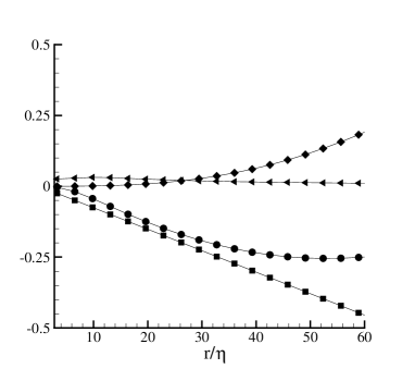
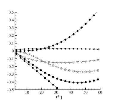
FIG. 5.: Scale by scale budget for the Newtonian (top) and the viscoelastic case (bottom). Symbols are defined in the text.

Newtonian and the polymeric contributions. The slope is then substantially larger than in the Newtonian case displayed on the top. Not unexpectedly, the global flux term is qualitatively similar to the corresponding Newtonian one, with a substantial range of scales where the linear trend defined by $F$ is reasonably well reproduced by $\Phi$. This emerges quite clearly from the plots in figure 6 where the budgets for Newtonian and viscoelastic turbulence are superimposed the one to the other, after a rescaling proportional to the respective values of the global dissipation. Also for the polymers, we are in presence of a direct cascade, with a negative global flux.

Returning to the plots on the bottom of figure 5, the most interesting feature is represented by the open symbols, circles and squares, which give the splitting of the flux into the classical contribution associated to the third order velocity structure function, $\Phi_{c}$ (circles), and to the polymer contribution, $\Phi_{p}$ (triangles), respectively. The larger scales are less affected by the polymers, with $\Phi_{p}$ becoming sub-leading with respect to $\Phi_{c}$. One may conjecture that, at sufficiently large scale and for Reynolds numbers large enough, the turbulence scalings are substantially unaffected by the polymers. Under this assumption, we see that the total dissipation $\bar{\epsilon}_{T}$ may be taken to measure a purely inertial energy transfer at large scales. This attaches to our conventional definition of Kolmogorov scale the obvious meaning of the length-scale where dissipation would occur in the absence of polymers.

Within the scenario according to which the large scales are unaffected by the polymers, the time criterion of Lumley [18] fixes the scale $r^{*}$ below which the polymers begin to feel the turbulent fluctuations. This happens when the eddy-turnover time of classical turbulent eddies, i.e. without the effect of the viscoelastic reaction, equals the principal relaxation time of the polymer chains. Assuming Kolmogorov scaling for the velocity increments, this leads to

$$r^{*} = (\bar{\epsilon}_{T}\,\tau^{3})^{1/2}$$ (41)

or, scaled with the conventional Kolmogorov length, to

$$r^{*}/\eta_{T} = \tau^{3/2}\,(\bar{\epsilon}_{T}/\nu_{T})^{3/4}\,.$$ (42)

From the data given in table I, for our simulation we have $r^{*}/\eta_{T}\simeq 70$, within a computational box of $l_{x}/\eta_{T}\simeq 174$, suggesting that the forcing, applied to the first shell of wavenumbers, acts just above the scale where the polymers already feel the turbulent fluctuations. In fact, a better way to apply the time criterion is to identify the eddy-turnover time as function of separation from the actual data provided by the DNS. This is done in figure 7, where as characteristic time for the scale $r$ we assume $r/\Phi_{c}^{1/3}$. From the figure we infer that our viscoelastic turbulence achieve an eddy-turnover time comparable with the viscoelastic relaxation time, horizontal line in the figure, at a scale considerably smaller then predicted on purely dimensional grounds, leaving a reasonable range of between the forcing and Lumley scale.

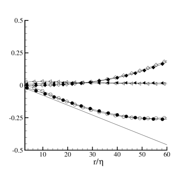
FIG. 6.: Re-scaled budget for the Newtonian (open symbols) and the viscoelastic (filled symbols).

Coming back to our comparison between the two components of the flux, at small scales we find that the component originated by the polymers takes over, entailing the reduction of the third-order structure function. The two curves, open circles and squares, clearly identify a cross-over scale $\ell_{p}$ according to the equation

$$\Phi_{p}(\ell_{p})\,=\,\Phi_{c}(\ell_{p})\,.$$ (43)

For our case the balance is achieved at $r/\eta_{T}\simeq 22$, while $\lambda/\eta_{T}=33$. Observe for comparison that, in the corresponding Newtonian case, $\lambda/\eta$ is about half the value. By inspection of the figure, we also find that all along the available range of scales the polymers reaction is dynamically relevant for the turbulent fluctuations, with $\Phi_{p}$ always comparable in magnitude with $\Phi_{c}$.

Dimensionally, the right-hand side of eq. (43) can be estimated as $\bar{\epsilon}_{T}\,\ell_{p}$, as follows by roughly assuming a purely classical inertial scaling for $r\geq\ell_{p}$. On the other hand, $\Phi_{p}(\ell_{p})$ should be somehow proportional to $\sigma^{**}\,\nu_{p}/\tau\,\bar{\epsilon}_{T}^{1/3}\,\ell_{p}^{1/3}$, where, again, Kolmogorov scaling is used to estimate $\delta V$ in eq. (40). Accounting for the constitutive relation (2), $T^{*}$ is expressed in terms of the, as yet, undetermined factor $\sigma^{**}$ which should account for the level of stretching achieved in the polymers at the cross-over scale. This yields the expression

$\displaystyle\ell_{p}=\frac{(\sigma^{**}\,\nu_{p}/\tau)^{3/2}}{\bar{\epsilon}_{T}}\,,$

which can be used to build the dimensionless quantity

$$\sigma^{**} = \tau/\nu_{p}\,(\ell_{p}\bar{\epsilon}_{T})^{2/3}\,.$$ (44)

For the present case we have ${(\nu_{p}/\tau)^{3/2}}/{\bar{\epsilon}_{T}}\simeq 1.4\,10^{-5}$, which, after considering that $\ell_{p}/\eta_{p}\simeq 22$,

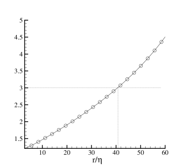
FIG. 7.: Eddy-turnover time, $r/\Phi_{c}^{1/3}$, vs scale $r$. The horizontal line corresponds to the relaxation time, $\tau$.

yields $\sigma^{**}\simeq 1400$. The parameter $\sigma^{**}$ allows to quantify the effective stretching of the chains at cross-over by assuming $\sigma^{**}\propto f^{**}R^{**}_{kk}/\rho^{2}_{0}$, see eq. (2).

The quantity

$$\sigma=f(R_{kk};\rho_{max},\rho_{0})R_{kk}/\rho^{2}_{0}$$ (45)

is plotted versus the elongation $R_{kk}/\rho^{2}_{0}$ on the right of figure 8. We see clearly the finite extensibility effect, with the unbound growth of $\sigma$ as the critical extension $\rho^{2}_{max}/\rho^{2}_{0}$ is approached from the left. Note that, at small elongation, $\sigma$ goes almost linearly with $R_{kk}/\rho^{2}_{0}$. The horizontal line plotted in the figure corresponds to the value $\sigma^{**}$ we have estimated from the numerical simulation. The intercept of this line with the curve representing $\sigma$ lays relatively far from the critical extension, though well within the region of non-linear elastic response.

It may be instructive to compare the elongation associated to the cross-over scale to the pdf of $R_{kk}/\rho^{2}_{0}$.

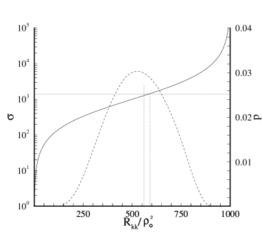
FIG. 8.: $\sigma$, see eq. (45), vs. polymers elongation, $R_{kk}/\rho_{0}^{2}$.

To this purpose, we superimpose to the plot of $\sigma$ given in figure 8 the histogram of the elongation as obtained by the numerical simulation. The effective elongation at cross-over, denoted by the vertical line, lies to the right of the maximum of the histogram, indicating a level of stretching substantially larger then either the most probable or the average elongation. Clearly the estimate here proposed should be understood as an order of magnitude analysis, to allow the comparison of different flow conditions.

To complete the analysis, in figure 9 we address the Yaglom-like equation for the free-energy. As seen in the top part of the figure, the left and the right hand side of eq. (34) balance within the accuracy of the available statistics.

The fluctuations of excess-power are converted into a free-energy flux with a negative sign, as wee see from the figure. Hence, also for the microstructure, we are in presence of a direct cascade. We like to stress that the direction of the cascade is not a priori obvious in this case, since we miss the standard term, linear in the

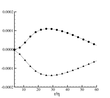
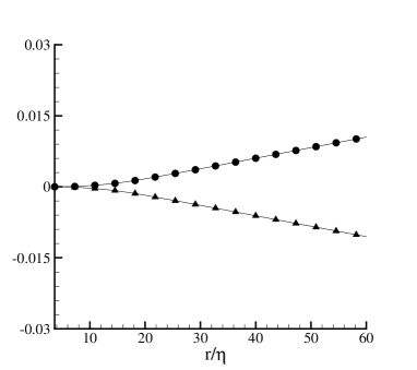
FIG. 9.: Top: The free-energy flux (filled triangles), and the forcing term given by the excess-power (filled circles) according to Yaglom equation. Bottom: The two contributions to the excess-power term in the Yaglom equation, stress-power term (filled circles) and polymeric dissipation term (filled triangles).

separation and related to the dissipation of the scalar, which usually determines the sign of the energy flux.

From the figure, the free-energy flux,

$\displaystyle\Phi_{a}\,=\,<\delta a^{2}\,\delta V_{\parallel}>\,,$

manifests a pronounced minimum in correspondence with the cross-over scale $\ell_{p}$, suggesting that, near cross-over the activity of the polymers is particularly intense and the polymers tend to become less active as the scale is increased. The bottom part of the figure gives the decomposition of the right-hand side of equation (34), with the positive term

associated to the stress power denoted by filled squares and that associated with the polymeric dissipation indicated by the filled triangles.

Order of magnitude considerations confirm that the data shown in the bottom part of figures 5 and in figure 9 are consistent. At cross-over, $r=\ell_{p}$, we find from figure 5 that $\Phi^{**}_{c}\simeq<\delta{V^{**}}^{3}>\simeq.12$, suggesting $\delta V^{**}\simeq.5$. From figure 9 we also have $<\delta{a^{**}}^{2}\delta V^{**}>\simeq.00015$. It follows $\delta a^{**}\simeq.017$ a value considerably close to $\delta{V^{**}}^{2}\simeq.025$. In other words, at the cross-over scale fluctuations of free-energy, or more loosely of elastic energy, and fluctuation of turbulent kinetic energy become comparable, as it should be expected.

VII Concluding remarks

The interaction between long chain polymers in dilute solution and turbulence is known to have a profound influence on the structure of turbulence. Several possible explanations have been proposed, with the eventual aim to understand the drag reducing properties manifested by such fluids in wall bounded turbulent flows. Even the most powerful approach, however, has to face the elusive mechanism by which polymers dynamics and turbulence are mutually coupled. Among others, specially noteworthy is the theory of De Gennes and Tabor, who proposed a cascade model for the viscoelastic turbulence of dilute polymers solutions. Their elegant theory issues from considering homogeneous isotropic conditions and rests upon suitable assumptions on the self-similar stretching of polymers chains under a fluctuating velocity field. The entire model is essentially phenomenological in nature, and should thus be contrasted with experimental observations.

In this context, we believe to have provided here a reasonable framework based on two essential ingredients. The first ingredient is the direct numerical simulation of the natural flow where the cascade issue should be addressed, namely homogeneous isotropic turbulence numerically modeled as a triply-periodic box with random forcing at large scales. Beside the obvious implementation in terms of spectral algorithms, this step required the selection of a good rheological model for the polymers. Based on previous experience, our natural choice has been the FENE-P model, known to capture reasonably well the drag-reducing effects still maintaining an affordable level of computational complexity.

The second ingredient is the extension to viscoelastic fluids of two of the, let’s say, few exact results known in classical turbulence theory, namely the Karman-Howarth equation for the velocity and the Yaglom equation for scalars. As a characteristic feature of viscoelastic turbulence, the coupling between velocity and extra-stress in the Karman-Howarth equation prevents recasting the result in the familiar form involving only longitudinal structure functions. Hence we have adopted a natural generalization in terms of suitable surface and volume integrals in the space of separations. Concerning the microstructure, the descriptor field is a second order tensor, making the derivation of the appropriate equation exceedingly cumbersome. We decided then to fucus our attention on the single most important scalar quantity, namely the free-energy, whose Yaglom-like equation follows straightforwardly.

The scale by scale budget based on the Karman-Howarth and Yaglom equation has been used to understand the respective role of the traditional energy transfer term versus polymeric transfer. We find a direct cascade occurring both in the kinetic field and in the microstructure, for which, as already discussed, the sign of the energy flux is not a priori obvious.

The budget has allowed us to identify a cross-over scale below which the polymers contribution becomes dominant, being sub-leading with respect to inertial transfer at larger scales. This is the analogous of the scale defining the elastic limit in the theory of De Gennes and Tabor. It is here derived in a rigorous context, and evaluated on the basis of a direct numerical simulation of a drag-reducing visco-elastic material as described by the FENE-P model.

We find that the polymers substantially deplete the energy content of the smallest scales, in agreement with recent experimental results, but they affect the dynamics of the fluctuations at all the scales of our simulation. The latter effect could be interpreted as an artifact of the limited extension of our computational domain which forced us to apply the external excitation relatively close to the scale defined by Lumley’s time criterion. Nonetheless the present results make questionable the existence of a purely passive range, where polymers are deformed without back-reaction on the velocity field.

Based on the balance of terms appearing in the exact form of the Karman-Howarth equation we have proposed a dimensionless parameter which may give a quantitative measure of the stretching the polymers experience at cross-over, when elastic effects become comparable with the corresponding kinetic energy.

Finally, a substantial level of intermittency is observed in the system, with fluctuations in turbulent kinetic energy considerably larger than usually observed in homogeneous isotropic turbulence of Newtonian fluids. This effect is presumably associated with the existence of the additional mechanism of energy removal from the scales of the forcing. In particular, a substantial part of the energy income does not follow the classical route cascading towards viscous dissipation. Instead, it is moved to the microstructure, to feed an additional cascade process seemingly requiring a larger level of fluctuations.

REFERENCES

- [1] Balkovsky, E., Fouxon, A., Lebedev, V., 2000, Turbulent dynamics of polymer solutions, Phys. Rev. Lett. 84 (20): 4765-4768.
- [2] Bird, R.B, Curtiss, C.F., Armstrong, R.C., Ole Hassager, 1987, Dynamics of polymeric liquids, vol. II Kinetic theory, Weyley-Interscience.
- [3] Cadot, O., Bonn, D., Douady, S., 1998, Turbulent drag reduction ina closed flow system: Bounday Layer versus bulk effects, Phys. Fluids 10(2) 426-436.
- [4] Casciola, C.M., Gualtieri, P., Benzi, R., Piva, R., 2002, Scale by scale budget and similarity laws for shear turbulence, submitted to J. Fluid Mech.
- [5] Chong, M.S., Perry, A.E., Cantwell, B.J., 1990, A general classification of three dimensional flow fields, Phys. Fluids A2 765-777.
- [6] De Angelis, E., Casciola, C.M., Piva, R., 1999, Dilute polymers and coherent structures in wall turbulence, in Rehology and fluid mechanics of nonlinear meterials, Siginer, D.A. ed., ASME.
- [7] De Angelis, E., Casciola, C.M., Piva, R., 2002, DNS of wall turbulence: dilute polymers and self-sustaining mechanisms, Computers and Fluids 31/4-7, 495-507.
- [8] De Angelis, E., Casciola, C.M., Mariano, P.M., Piva, R., 2002, Microstructure and turbulence in dilute polymer solutions, in Advances in multifield theories of continua with microstrucutre, Capriz, C. and Mariano, P.M. eds., Birkhauser.
- [9] De Gennes, P.G. 1986, Towards a scaling theory of drag reduction, Physica 140A, 9-25.
- [10] van Doorm, E., White, C.M., Sreenivasan, K.R., 1999, The decay of grid turbulence in polymer and surfactant solutions, Phys. Fluids 11(8) 2387-2393.
- [11] Friehe, C.A., Schwrtz, W.H. 1970, Grid-generated turbulence in dilute polymer solutions, J. Fluid Mech.44 173.
- [12] Frisch, U., 1995, Turbulence, Cambridge University Press.
- [13] Gualtieri, P., Casciola, C.M., Benzi, R., Amati G. and Piva, R., 2002, Scaling laws and intermittency in homogeneous shear flow, Phys. Fluids, 14(2), 583-596.
- [14] Hinze, O.J., 1959, Turbulence, MacGraw-Hill, New York.
- [15] Ilg, P., De Angelis, E., Karlin, I.V., Casciola, C.M., Succi, S., 2002 Polymer dynamic in wall turbulent flows, Europhys. Lett. 58(4), 616-622.
- [16] Luchik T.S., Tiederman W.G., 1987, Turbulent structure in low-concentration drag-reducing channel flows, J. Fluid Mech.190 241-263.
- [17] Lumley, J.L., 1969, Drag reduction by additives, Ann. Rev. Fluid Mech. 1 367.
- [18] Lumley, J.L., 1973, Drag reduction in turbulent flow by polymer additives, J. Pol. Sci., Macrom. Rew. 7 263-290.
- [19] Mini, T., Yoo, J.Y., Choi, H., 2001, Effect of spatial discretization schemes on numerical solutions of viscoelastic fluid flows , J Non-Newtonian Fluid Mech. 100(1-3) 27-4.
- [20] Mcomb, W.D., Allan, J., Greated, A., 1977, Effect of polymer additives on the small scale structure of grid generated turbulence, Phys. Fluids 20, 6873.
- [21] Monin, A.S., Yaglom, A.M., 1975, Statistical fluid mechanics: mechanics of turbulence, vol. II, MIT press.
- [22] Oberlack, M. 2001 A unified approach for symmetries in plane parallel turbulent shear flows J. Fluid Mech. 427, 299–328.
- [23] Sreenivasan, K.,R., White, C.M., 2000, The onset of drag reduction by dilute polymer additives, and the maximum drag reduction asymptote J. Fluid Mech. 409, 149-164.
- [24] Sureskumar, R., Beris, A.N., Handler, A.H., 1997, Direct numerical simulation of the turbulent channel flow of a polymer solution, Phys. Fluids 9(3), 743-755.
- [25] Wedgewood, L.E. and Bird, R.B., 1988, From molecular models to the solution of flow problems, Ind. Eng. Chem. Res.27 1313-1320.
- [26] Warholic, M.D., Massah, H., Hanratty, T.J., 1999, Influence of drag-reducing polymers on turbulence: effects of Reynolds number, concentration and mixing, Exp. Fluids 27 461-472.