Demonstration of the stability or instability of multibreathers at low coupling

Abstract

Whereas there exists a mathematical proof for one–site breathers stability, and an unpublished one for two–sites breathers, the methods for determining the stability properties of multibreathers rely in numerical computation of the Floquet multipliers or in the weak nonlinearity approximation leading to discrete non–linear Schrödinger equations. Here we present a set of multibreather stability theorems (MST) that provides with a simple method to determine multibreathers stability in Klein–Gordon systems. These theorems are based in the application of degenerate perturbation theory to Aubry’s band theory. We illustrate them with several examples.

1 Introduction

Discrete breathers are time–periodic, localized oscillations in discrete systems due to a combination of nonlinearity and discreteness. They have become a well understood phenomenon since the publication of the proof of existence in Ref. [1]. This proof is the origin of exact and powerful numerical methods to calculate them and to determine their stability [2]. A deeper insight has been achieved since the introduction of Aubry’s band theory [3]. The last reference, together with Ref. [4] can be considered as reviews, although a new one is badly needed after the huge development of the subject in the last years.

The stability of one–site breathers is proofed in Refs. [2, 3] under rather general conditions, the stability of the possible two–sites breathers in analyzed in an unpublished theorem in Ref. [5], page 69. Other methods use the hypothesis of small amplitude oscillations or the rotating wave approximation [6, 7] leading to the Nonlinear Schrödinger equation (DNLS), which is the actual equation analyzed, and, there are, of course, the efficient but slow numerical methods mentioned above.

Here we propose a method based in the properties of the bands in Aubry’s bands theory and perturbation theory, to obtain the stability properties of any multibreather at low coupling. In many cases it involves only some modification of the coupling matrix and the knowledge of the hardness/softness of the on–site potential. We will briefly summarize the band theory in the next section, while we introduce the notation and some basic concepts, on which our theory is based. However, we refer to Ref. [3, 1, 5] for detailed explanations, as it will be long and repetitive to expose it in detail.

In section 3 we develop the method for symmetric on–site potentials or in–phase multibreathers, which is synthesized in a theorem, commented in section 4. Its scope is enlarged to non–symmetric potentials in section 3, and to generalized Klein–Gordon systems in section 6. The method is applied to several interesting examples in sections 7 and 8. In Appendix A we calculate the value of a magnitude $\gamma$ used in our theory, and in Appendix B we relate the curvature of the bands with the characteristics of the on site potential.

2 Band theory and notation

2.1 The Newton operator

We consider Klein–Gordon systems with linear coupling described by dynamical equations of the form:

$$\ddot{u}_{n}\,+\,V^{\prime}(u_{n})\,+\,\varepsilon\,\sum_{m=1}^{N}\,C_{n\,m}u_{n}\,=\,0\,\quad n=1,\dots,N$$ (1)

where the variables $u_{n}$ are functions of time $t$, $V(u_{n})$ is an homogeneous on–site potential, $V^{\prime}$ its derivative, $\dot{u}_{n}$ denotes derivation with respect to time, $N$ is the number of oscillators, $C$ is a coupling constant matrix, which can describe nearest neighbor or long–range interaction, and includes the boundary conditions, and $\varepsilon$ is the coupling parameter. We use a notation similar to quantum mechanics, i.e., $|u\rangle\,\equiv[u_{1}(t),\dots,u_{N}(t)]^{\dagger}$ (^† meaning the transpose matrix). Defining $V(u)=[V(u_{1}),\dots,V(u_{N})]^{\dagger}$ and analogously its derivatives, equation (1) can be written as:

$$|\ddot{u}\rangle\,+\,|V^{\prime}(u)\rangle\,+\,\varepsilon\,C\,|u\rangle\,=\,0\,.$$ (2)

We suppose that the functions $u_{n}(t)$ are time–periodic (with period $T$ and frequency $\omega_{\mathrm{b}}$), time–reversible solutions and, therefore, they can be written as cosine Fourier series with real coefficients (some of these assumptions will be relaxed later). The (linear) stability properties of a given solution $|u\rangle$ depend on the properties of the characteristic equation for the Newton operator $\mathcal{N}_{\varepsilon}$ given by

$$\mathcal{N}_{\varepsilon}(u)\,|\xi\rangle\,\equiv\,|\ddot{\xi}\rangle\,+\,V^{\prime\prime}(u)\cdot|\xi\rangle\,+\,\varepsilon\,C\,|\xi\rangle=\,E\,|\xi\rangle\,,$$ (3)

where $\cdot$ product is the list product, i.e., $f(u)\cdot|\xi\rangle$ is the column matrix with elements $f(u_{n}(t))\,\xi_{n}(t)$. If $E=0$, this equation describes the evolution of small perturbations $|\xi\rangle$ of $|u\rangle$.

2.2 The Floquet matrix

Any solutions of Eq. (3) can be determined by the column matrix of the initial conditions for positions and momenta $\Omega(0)=[\xi_{1}(0),\dots\xi_{N}(0),\pi_{1}(0),\dots\pi_{N}(0)]^{\dagger}$, with $\pi_{n}(t)=\dot{\xi}_{n}(t)$, and $\Omega(t)$ describes its evolution in the space of coordinates and momenta. A base of solutions is given by the $2\,N$ functions with initial conditions $\Omega^{\nu}(0)$, $\nu=1,\dots,2\,N$, with $\Omega^{\nu}_{l}(0)=\delta_{\nu\,l}$. We will identify often a given solution $\xi(t)$ of the Newton equation with the corresponding matrix of initial conditions $\Omega(0)$. As the Newton operator depends on the $T$–periodic solution $u(t)$, it is also periodic, and the evolution of the solutions of Eq. (3) can be studied by means of the Floquet operator, which maps $\xi(t)$ into $\xi(t+T)$. In a finite system this is equivalent to the Floquet matrix $\mathcal{F}_{E}$ being given by:

$$\left[\begin{array}[]{c}\{\xi_{n}(T)\}\\ \{\pi_{n}(T)\}\end{array}\right]=\mathcal{F}_{E}\,\left[\begin{array}[]{c}\{\xi_{n}(0)\}\\ \{\pi_{n}(0)\}\end{array}\right]\,$$ (4)

These matrices can be easily constructed numerically, by integrating Eq. (3) $2\,N$ times from $t=0$ to $t=T$, with initial conditions $\Omega^{\nu}(0)$. Then, the $\nu$ column of $\mathcal{F}_{E}$ is given by $\Omega^{\nu}(T)$.

2.3 Stability and bifurcations

The eigenvalues $\{\lambda_{l}\}_{l=1}^{2\,N}$ of $F_{0}$, called the Floquet multipliers, determine the linear stability of the solution $u(t)$. If there is any eigenvalue with $|\lambda_{l}|>1$, the corresponding eigenfunction $\xi^{l}(t)$ grows with time and $u(t)$ is unstable; if $\lambda_{l}=1$, $\xi^{l}(t)$ is $T$-periodic; if $\lambda_{l}=-1$, $\xi^{l}(t)$ is $2\,T$–periodic. However, $F_{0}$ (and any $F_{E}$) is a symplectic matrix, as it is derived from the symplectic system Eq. (3), which implies that if $\lambda_{l}$ is a non–zero eigenvalue, so it is $1/\lambda$. $F_{E}$ is also real, which in turn implies that $\lambda_{l}^{*}$ and $1/\lambda^{*}$ are also multipliers. Therefore, the eigenvalues of $F_{E}$ come in groups of four, if they are not real, or in pairs, if they are real or if $|\lambda_{l}|=1$. We can write the Floquet multipliers as $\{\exp(\mathrm{i}\theta_{l})\}$, with $\theta_{l}$, in general, complex numbers. The complex number $\mathrm{i}\theta_{l}$ are called the Floquet exponents, and $\theta_{l}$ the Floquet arguments.

The only possibility for the stability of $u(t)$ is that all the eigenvalues of $F_{0}$ have moduli $1$, i.e., they are at the unit circle. Therefore, the condition for linear stability of $u(t)$ can be described as all the Floquet arguments for $F_{0}$ being real. Moreover, if $u(t)$ is stable and, then, every $|\lambda_{l}|=1$, the Floquet multipliers come in complex conjugate pairs with arguments $(\pm\theta_{l})$ or as double $1$ or $-1$ ($\theta=0$ or $\theta=\pm\pi$). If a parameter like the coupling $\varepsilon$ is changed the multipliers of $F_{0}$ change continuously. Therefore, a bifurcation to an unstable solution can only take place in three different forms: a) Harmonic instability: two complex eigenvalues moving along the unit circle collide at $\lambda=1$ ($\theta=0$); b) Subharmonic instability: two complex eigenvalues moving along the unit circle collide at $\lambda=-1$ ($\theta=\pm\pi$); c) Oscillatory or Hopf instability: two pairs of complex eigenvalues moving along the unit circle collide at $\pm\theta\neq 0$ and abandon the unit circle as a quadruplet $(\lambda,1/\lambda,\lambda^{*},1/\lambda^{*})$.

A Floquet multiplier of $F_{0}$ is always known. Calculating the derivative of Eq. (2) with respect to time we obtain that $\mathcal{N}\,\dot{u}=0$. $\dot{u}$ is also $T$–periodic, therefore, it is an eigenfunction of $F_{0}$ with multiplier $1$, and as they come in pairs, there is always a double $1$ multiplier. $\dot{u}$ is called the phase mode because its meaning is that if $\dot{u}(t)$ is a solution of Eq. (2), $\dot{u}(t+dt)$ is also a solution. While the solution $u(t)$ exists, this double eigenvalue is always there. Due to the possible forms of the bifurcations, if all the multipliers are isolated except the double $1$, the system is structurally stable, i.e., there is a neighborhood in the space of the parameters where $u(t)$ is stable.

2.4 Aubry’s band theory

However, it turns out that much information can be obtained by studying also the Floquet arguments for $E\neq 0$, with is known as Aubry’s band theory [3]. The set of points $(\theta,E)$, with $\theta$ a real Floquet argument of $F_{E}$ have a band structure. The fact that the Floquet multipliers come in pairs of complex conjugate pairs brings about that if $(\theta,E)$ belongs to a band, $(-\theta,E)$ does it too, i.e., the bands are symmetric with respect to $\theta$ and $\d E/\d\theta(0)=0$. As $\dot{u}$ has eigenvalue $1$ ($\theta=0$), there is always a band tangent to the axis $E=0$ at $\theta=0$. There are at most $2\,N$ points for a given value of $E$ and, therefore, there are at most $2\,N$ bands crossing any horizontal axes in the space of coordinates $(\theta,E)$. The condition for linear stability of $u(t)$ is equivalent to the existence of $2\,N$ bands crossing the axis $E=0$ (including tangent points with their multiplicity). If a parameter like the coupling $\varepsilon$ changes, the bands evolve continuously, and they can loss crossing points with $E=0$, bringing about the instability.

We know more about the eigenfunctions of the Newton operator. The fact that it is periodic, or, in other words, that it commutes with the operator $\mathcal{P}$ of translation in time a period, $\mathcal{P}f(t)=f(t+T)$, implies that its eigenfunctions can be chosen simultaneously as eigenfunctions of $\mathcal{P}$, which by Bloch theorem, are given by $\xi(\theta,t)=\chi(\theta,t)\,\exp(\mathrm{i}\,\theta\,t/T)$, $\chi(\theta,t)$ being a column matrix of $T$–periodic functions. It is straightforward to check that $\exp(\mathrm{i}\theta)$ is the corresponding Floquet multiplier, and $\theta$ its Floquet argument ($F_{E}$ is simply the representation of $\mathcal{P}$ in the base $\Omega^{l}$).

2.5 Bands at the anticontinuous limit

The key concept on the demonstration of breather existence [1], single breather stability [3] and the present paper is the anticontinuous limit, i.e., the system with all the oscillators uncoupled, $\varepsilon=0$, in Eq. (1–2). At the anticontinuous limit, Eq. (1) reduces to $N$ identical equations:

$$\ddot{u}_{n}\,+\,V^{\prime}(u_{n})\,=\,0\,.$$ (5)

Supposing that we consider time–reversible solutions around a single minimum of $V$, there are only three different solutions: a) oscillators at rest $u_{n}\,=\,0$; b) excited oscillators with identical $u_{n}(t)$, hereafter denoted $u^{0}(t)$; c) excited oscillators with a phase difference of $\pi$ with the previous ones, given by $u_{n}(t)\,=\,u^{0}(t\,+\,T/2)$. Each site index is given a code $\sigma_{n}$, which takes elements in $\{0,1,-1\}$, where $\sigma_{n}\,=\,0$ represents an oscillator at rest, $u_{n}\,=\,0$; $\sigma_{n}\,=\,1$, an oscillator with solution $u^{0}(t)$; and $\sigma_{n}\,=\,-1$, the solution $u^{0}(t+T/2)$. The matrix of codes $\sigma\,=\,[\sigma_{1},\dots,\sigma_{N}]^{\dagger}$ represents the state of the system at the anticontinuous limit.

We suppose that there are $p$ oscillators at rest and $N\,-\,p$ excited oscillators. Equation (3) at $\varepsilon\,=\,0$ becomes

$$\mathcal{N}_{0}(u)\,|\xi\rangle\,\equiv\,|\ddot{\xi}\rangle\,+\,V^{\prime\prime}(u)\cdot|\xi\rangle\,=\,E\,|\xi\rangle\,,$$ (6)

or, equivalently, $N\,-\,p$ identical equations:

$$\ddot{\xi}_{n}\,+\,V^{\prime\prime}(u_{n})\,\xi_{n}=\,E\,\xi_{n}\,,$$ (7)

with only a periodic eigenfunction for $E\,=\,0$, the phase mode $\dot{u}_{n}(t)$ for the isolated, excited oscillators. The other one is the growth mode, (see Appendix B) which is not bounded and will not be used in this work. They give rise to $N-p$ bands tangent to the axis $E\,=\,0$, shown in Fig. 1. They have positive curvature at $(\theta,E)=(0,0)$ if the on–site potential is soft ($\d H/\d\omega_{b}<0$) and negative if it is hard ($\d H/\d\omega_{b}>0$), as it is demonstrated in Appendix B. The possibility of $\d H/\d\omega_{b}=0$ is excluded by the conditions of the breather existence theorem [1], which means that the on-site potential is truly nonlinear for the isolated oscillators with the breather frequency $\omega_{\mathrm{b}}$. If, as we are supposing here, the on–site potentials $V(u_{n})$ are identical, the solutions $u_{n}(t)$ are also identical except for a change of phase and the bands are superposed, if not, we might have different bands but with the same general shape.

The remaining $p$ equations corresponding to the oscillators at rest are of the form:

$$\ddot{\xi}_{n}\,+\,(\omega_{0})^{2}\xi_{n}=\,E\,\xi_{n}\,,$$ (8)

with $\omega_{0}\,=\,\sqrt{V^{\prime\prime}(0)}$. They have only a $T$-periodic solution for $E\,=\,0$ , the null solution, due to the non–resonance condition for breather existence $n\omega_{b}\,\neq\,\omega_{0}$ ($p\in\mathbb{N}$) [1], i.e., none of the harmonics of the breather resonates with the oscillators at rest. They provide $p$ identical bands which are easily calculated solving the equation above. Its solutions are $\xi=\exp(\pm\mathrm{i}\sqrt{\omega_{0}^{2}-E}\,\,t)$, with Floquet multipliers $\exp(\pm\mathrm{i}\sqrt{\omega_{0}^{2}-E}\,\,T)$ and Floquet arguments $\theta=\pm\sqrt{\omega_{0}^{2}-E}\,\,T$. That is, the bands are given by $E=\omega_{0}^{2}-\omega_{\mathrm{b}}^{2}(\theta/T)^{2}$, where $\theta$ can be reduced to the first Brillouin zone $[-\pi,\pi]$ by the addition of $2\pi p$, $p\in\mathbb{Z}$. If the oscillators have different rest frequencies, the rest bands are not superposed but they have the same characteristics.

The rest bands are also shown in Fig. 1. Note that this figure is only a sketch, for clarity, as very often some excited oscillators bands are very flat and difficult to appreciate at the same scale. This sketch reproduces, however, the basics facts of the band structure.

When the coupling is switched on, the degeneracy of the bands is generically raised. All the tangent bands at $(\theta,E)=(0,0)$ except one, than continues there, move upwards or downwards. If the on–site potential is soft, Fig. 1 (left), and a band moves upwards, a double tangent point with the axis $E=0$ is lost, or, in other terms, a pair of Floquet arguments of $F_{0}$ becomes complex and the solution $u(t)$ is unstable. If the on site potential is hard, Fig. 1 (right), the same occurs when a band moves downwards.

3 Multibreathers stability

In this work use degenerate perturbation theory [8] to demonstrate the stability or instability of the breathers of any code. Degenerate perturbation theory establishes that if $\mathcal{N}_{0}$ is a linear operator with a degenerate eigenvalue $E_{0}$, with eigenvectors $\{|v_{n}\rangle\}$, which are ortonormal with respect to a scalar product, i.e., $\langle v_{n}|v_{m}\rangle\,=\,\delta_{n\,m}$, and if $\varepsilon\,\tilde{\mathcal{N}}$ is a perturbation of $\mathcal{N}_{0}$, with $\varepsilon$ small; then, to first order in $\varepsilon$, the eigenvalues of $\mathcal{N}_{0}\,+\,\varepsilon\,\tilde{\mathcal{N}}$ are $E_{0}\,+\varepsilon\,\,\lambda_{i}$, with $\lambda_{i}$ being the eigenvalues of the perturbation matrix $Q$ with elements $Q_{n\,m}\,=\,\langle v_{n}|\tilde{\mathcal{N}}|v_{m}\rangle$. Note that perturbation theory as described in the reference cited, is time independent perturbation theory, but our time variable $t$ is their spatial coordinate $x$.

Let us consider again Eq. (3) with zero coupling, $\varepsilon=0$. As explained in the previous section, if there are $N-p$ excited oscillators, there $N-p$ zero eigenvalues corresponding to the $T$–periodic eigenfunction $\dot{u}_{n}$ (the phase modes of the isolated oscillators), or in other words, a $N-p$ times degenerate eigenvalue $E_{0}=0$ if we restrict the domain of $\mathcal{N}$ to periodic functions. What we need to know is the sign of this degenerate eigenvalues when the coupling is switched on.

To apply degenerate theory to multibreather stability we need to identify the perturbation operator, a suitable scalar product and a ortonormal basis of the eigenspace with eigenvalue $E_{0}=0$. The scalar product is defined as:

$$\langle\xi_{1}|\xi_{2}\rangle\,=\,\sum_{n=1}^{N}\int_{-T/2}^{T/2}\xi_{1}^{*}(t)\xi_{2}(t)\,.\d t\,.$$ (9)

Let us suppose initially that all the excited oscillator are identical and vibrate in phase. We will denote by $u^{0}(t)$ these identical solutions. In this case, all the phase modes are also identical and will be denoted as $\dot{u}^{0}$. The $N-p$ elements of the basis are

$$|n\rangle\,=\,\frac{1}{\mu}[0,\dots,0,\dot{u}^{0},0,\dots,0]^{\dagger},$$ (10)

with the non-zero element at the position $n$, $n$ being the index of the excited oscillators, and $\mu\,=\,\sqrt{\int_{-T/2}^{T/2}(\dot{u}^{0})^{2}\,\d t}$. It is straightforward to check that they are ortonormal.

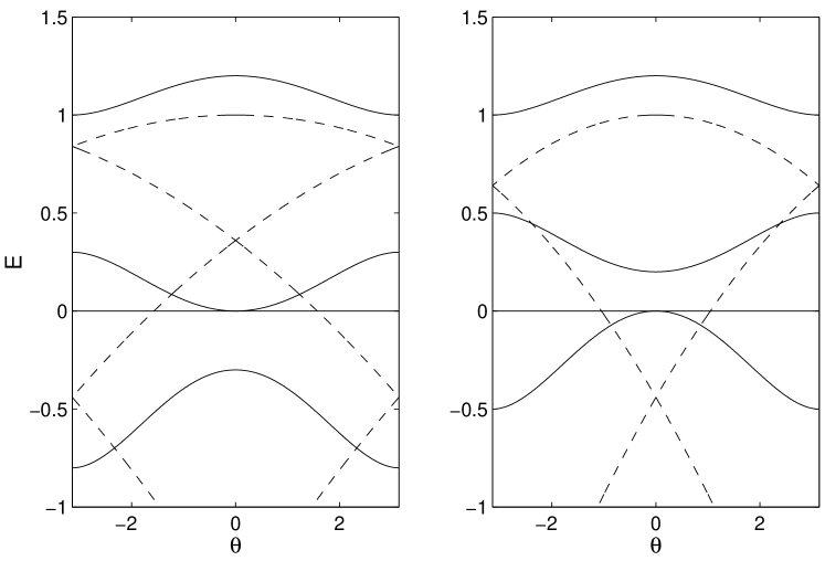
Figure 1: Sketch of the band structure for a soft on–site potential (left) and a hard on–site potential (right). The continuous lines correspond to excited oscillators and the dashed ones to oscillators at rest.

It is enough to know the eigenvalues corresponding to periodic and real solutions, i.e., with Floquet argument $\theta\,=\,0$, as the intersections of the bands with the axis $\theta\,=\,0$ correspond to periodic solutions of (3). Therefore the $N-p$ $|n\rangle$’s form the basis of the degenerate eigenvalue $E_{0}=0$ needed to apply perturbation theory.

To obtain the perturbation operator, we expand in Taylor series Eq. (3) at $\varepsilon\,=\,0$ and obtain to first order in $\varepsilon$ :

$$\mathcal{N}_{\varepsilon}(u)\,|\xi\rangle\, = \,|\ddot{\xi}\rangle\,+\,\,V^{\prime\prime}(u)\cdot|\xi\rangle\,+\,\varepsilon\,\big{(}\,V^{\prime\prime\prime}(u)\cdot u_{\varepsilon}\,\cdot|\xi\rangle\,+\,C\,|\xi\rangle\,\big{)}\,=$$ (11)

$$= \,(E_{0}\,+\,\varepsilon\,\lambda_{i})|\xi\rangle\,,$$

with $u_{\varepsilon}=\big{(}\frac{\displaystyle\partial u}{\displaystyle\partial\varepsilon}\big{)}_{\varepsilon=0}$ and $u$ is also the $\varepsilon=0$ solution.

Therefore the perturbation operator of $\mathcal{N}_{0}$ is

$$\tilde{\mathcal{N}}\,|\xi\rangle\,=V^{\prime\prime\prime}(u))\cdot u_{\varepsilon}\cdot|\xi\rangle\,+\,C\,|\xi\rangle\,,$$ (12)

where $u$ and $u_{\varepsilon}$ are calculated at $\varepsilon=0$. We do not know $u_{\varepsilon}$, but deriving with respect to $\varepsilon$, at $\varepsilon\,=\,0$, the dynamical equations (2) we obtain:

$$|\ddot{u}_{\varepsilon}\rangle\,+\,V^{\prime\prime}(u)\cdot|u_{\varepsilon}\rangle\,+\,C\,|u\rangle\,=\,0\quad\mbox{or}\quad N_{0}|u_{\varepsilon}\rangle\,=\,-C\,|u\rangle\,.$$ (13)

The perturbed eigenvalues $E_{i}$ are $\varepsilon\,\lambda_{i}$ , $\lambda_{i}$ being the eigenvalues of the perturbation matrix $Q$, with elements $\langle n|\tilde{\mathcal{N}}|m\rangle$. The matrix $\tilde{C}$ of elements $\langle n|C|m\rangle$ is simply the matrix $C$ without the columns and rows corresponding to the oscillators at rest. The other terms are:

$$\langle n|V^{\prime\prime\prime}(u)\cdot u_{\varepsilon}|m\rangle\,=$$

$$\frac{1}{\mu^{2}}\,\int_{-T/2}^{T/2}[\dots,0,\dot{u}_{n}^{0},0,\dots]\, [\dots,0,V^{\prime\prime\prime}(u^{0})\,u_{m,\varepsilon}\,\dot{u}_{m}^{0},0,\dots]^{\dagger}\,\d t\,=$$ (14)

$$\frac{\displaystyle\delta_{n\,m}}{\displaystyle\mu^{2}}\,\int_{-T/2}^{T/2}\dot{u}^{0}\,V^{\prime\prime\prime}(u^{0})\,u_{n,\varepsilon}\,\dot{u}^{0}\,\d t\,,$$

with $u_{n,\varepsilon}=\big{(}\frac{\displaystyle\partial u_{n}}{\displaystyle\partial\varepsilon}\big{)}_{\varepsilon=0}$. Thus, only the diagonal elements $\langle n|V^{\prime\prime\prime}(u)\cdot u_{\varepsilon}\cdot|n\rangle$ are non–zero. To calculate the last integral in (14) we will integrate by parts and use that the integral in a period of the derivative of a periodic function is zero. Besides, the functions $u_{n,\varepsilon}$ are periodic as the coefficients of their Fourier series are given by the derivatives with respect to $\varepsilon$ of the Fourier coefficients of $u_{n}$. In the deduction below, all the integral limits are $-T/2$ and $T/2$, and the terms between brackets from integration by parts will be zero. The last integral in Eq. (14) becomes:

$$\left[\dot{u}^{0}\,u_{n,\varepsilon}\,V^{\prime\prime}(u^{0})\right]_{-T/2}^{T/2}\,-\,\int\,V^{\prime\prime}(u^{0})\dot{u}^{0}\,\dot{u}_{n,\varepsilon}\,\d t\,-\,\int\,V^{\prime\prime}(u^{0})\,\ddot{u}^{0}\,u_{n,\varepsilon}\,\d t\, =$$

$$-\left[V^{\prime}(u^{0})\,\dot{u}_{n,\varepsilon},\right]_{-T/2}^{T/2}\,+\,\int\,V^{\prime}(u^{0})\,\ddot{u}_{\varepsilon,n},\d t\,-\int\,V^{\prime\prime}(u^{0})\,\ddot{u}^{0}\,u_{n,\varepsilon}\,\d t\, =$$

$$-\,\int\,\ddot{u}^{0}\,(\ddot{u}_{n,\varepsilon}\,+\,V^{\prime\prime}(u^{0})\,u_{n,\varepsilon})\d t\mbox{}$$ (15)

The term between parentheses, is the $n$ component of the lhs of Eq. (13), i.e., it becomes $-\sum_{m}C_{n\,m}\,u_{m}^{0}$, where $u_{m}^{0}\,=\,u^{0}$, if the oscillator $m$ is excited, and zero otherwise, i.e., it is $-\sum_{m}\tilde{C}_{n\,m}\,u^{0}\,=\,-(\sum_{m}\tilde{C}_{n\,m})\,u^{0}$. Equation (LABEL:eq:larga) becomes:

$$(\sum_{m}\tilde{C}_{n\,m})\,\int\,\ddot{u}^{0}\,u^{0}\,dt\, =$$

$$(\sum_{m}\tilde{C}_{n\,m})\,\left(\left[\dot{u}^{0}\,u^{0}\right]_{-T/2}^{T/2}-\int(\dot{u}^{0})^{2}\,dt\right)\, = \,-(\sum_{m}\tilde{C}_{n\,m})\mu^{2}\,.$$ (16)

That is, equation (14), leads to:

$$\langle n|V^{\prime\prime\prime}(u)\cdot u_{\varepsilon}\cdot|n\rangle\,=\,-\sum_{m}\tilde{C}_{n\,m}\quad\textrm{at}\quad\varepsilon\,=\,0\,.$$ (17)

Therefore the diagonal elements of the perturbation matrix $Q$ are

$$Q_{n\,n}=\,-\,\sum_{m}\,\tilde{C}_{n\,m}\,+\,\tilde{C}_{n\,n}\,=\,-\,\sum_{\forall\,m\neq n}\,\tilde{C}_{n\,m}\,=\,\sum_{\forall\,m\neq n}\,Q_{n\,m}\,.$$ (18)

To summarize, the perturbation matrix $Q$ is given by:

$$Q_{n\,m}\,=\,\tilde{C}_{n\,m},\quad n\neq m\quad,\quad Q_{n\,n}\,=\,-\,\sum_{\forall\,m\neq n}\,Q_{n\,m}\,,$$ (19)

$\tilde{C}$ being the coupling matrix without the $p$ rows and columns corresponding to oscillators at rest.

This result can be very easily extended, to the case when there are oscillators out of phase, at least for an even potential $V(u)$. In this case $u^{0}(t+T/2)\,=\,-u^{0}(t)$ and $\dot{u}^{0}(t+T/2)\,=\,-\dot{u}^{0}(t)$. Let us define a new code $\tilde{\sigma}$, which is equal to $\sigma$, but with $+1$ instead of zeros, and perform the ansatz $u_{n}=\tilde{\sigma}_{n}\,\tilde{u}_{n}$. By substitution in the dynamical equations (1), and taking into account that $V^{\prime}(u_{n})\,=\,V^{\prime}(\tilde{\sigma}_{n}\,\tilde{u}_{n})\,=\,\tilde{\sigma}_{n}\,V^{\prime}(\tilde{u}_{n})$, because $V^{\prime}(u)$ is odd, we obtain:

$$\tilde{\sigma}_{n}\,\ddot{\tilde{u}}_{n}\,+\,\tilde{\sigma}_{n}\,V^{\prime}(\tilde{u}_{n})\,+\,\sum_{m}\,C_{n\,m}\,\tilde{\sigma}_{m}\,\tilde{u}_{m}\,=\,0\,.$$ (20)

Multiplying by $\tilde{\sigma}_{n}$, and using that its square is $+1$ we get:

$$\ddot{\tilde{u}}_{n}\,+\,V^{\prime}(\tilde{u}_{n})\,+\,\sum_{m}\,\tilde{\sigma}_{n}\,C_{n\,m}\,\tilde{\sigma}_{m}\,\tilde{u}_{m}\,=\,0\,.$$ (21)

As the elements of $C$ with an index corresponding to an oscillator at rest will not appear in the calculations, we can define a new coupling matrix, with elements $\sigma_{n}\,C_{n\,m}\,\sigma_{m}$, i.e., $\textrm{Diag}(\sigma)\,C\,\textrm{Diag}(\sigma)$. The eigenvalues $E_{i}$ will have the right sign, but the eigenfunctions $\tilde{\xi}$ of the Newton operator corresponding to (21) have to be transformed to recover the original ones by $|\xi\rangle\,=\,\textrm{Diag}(\sigma)\,|\tilde{\xi}\rangle$

The result can be summarized in the following way:

Theorem 1 (Symmetric MST)

Consider a Klein–Gordon system, with homogeneous on–site potential $V$, linear coupling matrix $C$ and coupling parameter $\varepsilon$, and a multibreather given by a vector code $\sigma$ at zero coupling, with $p$ zero elements, and $N\,-\,p$ non–zero elements. The potential $V$ must be even if there is any $-1$ in $\sigma$. We define the following matrices: $S\,=\,\textrm{Diag}(\sigma)$; $\tilde{C}$ the $N\,-\,p$, squared matrix equal to $S\,C\,S$ but without the rows and columns corresponding to the zero codes in $\sigma$; $Q$, the perturbation matrix, with non–diagonal elements $Q_{n\,m}=\tilde{C}_{n\,m}$, and diagonal elements $Q_{n\,n}\,=\,-\sum_{\forall\,m\neq n}\tilde{C}_{n\,m}$. Let $\{\lambda_{i}\}_{i=1}^{N-p}$ be the eigenvalues of $Q$ and suppose that there is only one zero among them. Then:
a) if $V(u_{n})$ is hard and there is any negative value in $\{\varepsilon\,\lambda_{i}\}$ the multibreather at low coupling will be unstable, and stable otherwise.
b) if $V(u_{n})$ is soft and there is any positive value in $\{\varepsilon\,\lambda_{i}\}$ the multibreather at low coupling will be unstable, and stable otherwise.

There is always a zero eigenvalue is explained below. If there are more than one the stability is undefined within first order perturbation theory.

4 Comments

4.1 Global phase mode

The perturbation matrix $Q$ has always a zero eigenvalue corresponding to the global phase mode. It can be useful to make it apparent as it reduces the order of the secular equation by an unity. Considering the matrix $Z=Q-\lambda\,I$, $\det(Z)=0$ is the secular equation. Its roots are the same if we change $Z$ to $Z^{\prime}$ obtained by summing to the first column the rest of them, i.e., $Z^{\prime}_{n\,1}\,=-\sum_{\forall\,m\neq n}\tilde{C}_{n,m}\,-\lambda\,+\,\sum_{\forall\,m\neq n}\tilde{C}_{n,m}\,=\,-\lambda$. Now, subtracting the first row from the rest of them, the first column has only a non zero element, which is equal to $\-\lambda$. Therefore, $\lambda=0$ is an eigenvalue of $Q$ and the secular equation is reduced by an unity.

The corresponding eigenvector $\tilde{x}$ satisfies $Q\,\tilde{x}\,=\,0$, i.e., $-\,(\sum_{\forall\,m\neq n}\,\tilde{C}_{n\,m}\,)\,\tilde{x}_{n}\,+\,\sum_{\forall\,m\neq n}\,\tilde{C}_{n\,m}\,\tilde{x}_{m}\,=\,0$, $\forall n$, with solution $\tilde{x}_{n}\,=\,1$, $\forall n$. Therefore, $x\,=\,S\,\tilde{x}\,=\sigma$, which corresponds to the global phase mode.

4.2 Extended and reduced forms

Note that the code $\sigma$ is the matrix of components of the multibreather at zero coupling in a N–dimensional basis, $\{\,|n\rangle\}$, with the only non zero element $u^{0}$ at the position $n$, including the indexes of all the oscillators. For numerical calculation and interpretation of the eigenvalues and eigenvectors of $Q$ it can be more convenient to define $\tilde{C}\,=\,S\,C\,S$, i.e, conserving the rows and columns corresponding to the rest oscillators but all their elements set to zero. It will be denoted the extended form while the previous one is the reduced form. The price for using the extended form is to obtain $p$ extra zero eigenvalues, which causes no harm, except if there are more than $p+1$, as it can make more difficult the interpretation of the eigenvectors.

4.3 Diagonal elements

The diagonal elements of $C$ play no role, because they do not appear in the coupling matrix. Therefore a coupling of the spring–type as $\varepsilon\,(\,2\,u_{n}-\,u_{n-1}-\,u_{n+1})$ gives identical results as the dipole-type $-\varepsilon\,(u_{n-1}+u_{n+1})$.

4.4 2D and 3D lattices

Note that the theorem applies equally to 2D and 3D lattices, provided that we can number the sites with an index $n$, or consider $n$ as a multi–index, and construct the coupling matrix $C$.

5 Non–symmetric potentials

The extension to non–symmetric potentials $V(u_{n})$ is straightforward, but it involves some numerical or analytical calculation. That is the reason for not including it in theorem 1, and we present it here as another theorem instead. If the potential is non–symmetric, there are two time–symmetric, $T$-periodic solutions to the equations for the isolated oscillators at zero coupling, Eq. (5): $u^{0}(t)$, with code $+1$, and $u^{0}(t+T/2)$, which is no longer $-u^{0}(t)$, with code $-1$. The $N-p$ elements of the basis, $|n\rangle$ will be as in Eq. (10) but with $\dot{u}^{0}(t+T/2)$ instead of $\dot{u}^{0}(t)$ if $\sigma_{n}\,=\,-1$. Let us define the symmetry coefficient, $\gamma$, in the following way:

$$\gamma\,=\,-\,\frac{\int_{-T/2}^{T/2}\dot{u}^{0}(t)\,\dot{u}^{0}(t+T/2)\,\d t}{\int_{-T/2}^{T/2}\dot{u}^{0}(t)\,\dot{u}^{0}(t)\,\d t}$$ (22)

If $\{z_{k}\}_{k=0}^{k_{m}}$ are the Fourier coefficients of a $k_{m}$–truncated Fourier series of $u^{0}(t)$, i.e., $u^{0}(t)\,=\,z_{0}\,+\,\sum_{k=1}^{k_{m}}2\,z_{k}\,\cos(\,k\,\omega_{b}\,t)$, then:

$$\gamma\,=\,-\,\frac{\sum_{k=1}^{k_{m}}(-1)^{k}\,k^{2}\,z_{k}^{2}}{\sum_{k=1}^{k_{m}}\,k^{2}\,z_{k}^{2}}\,.$$ (23)

Note that $\gamma$ depends on the breather frequency through the $\{z_{k}\}$, and it is positive and smaller than $1$, being its value $\gamma\,=\,1$ for the symmetric potential case. Following the deduction of theorem 1 it is straightforward to obtain:

Theorem 2 (Non–symmetric MST)

The generalization of theorem 1 for non–symmetric potentials consists of constructing the perturbation matrix $Q$ in the following way:
a) If $n$ or $m$ are indexes corresponding to oscillators at rest $Q_{n\,m}\,=\,0$.
b) If $n$ and $m$, $n\neq m$, are indexes corresponding to excited oscillators in phase, i.e., $\sigma_{n}\,\sigma_{m}\,=\,1$, $Q_{n\,m}\,=\,C_{n\,m}$.
c) If $n$ and $m$, $n\neq m$, are indexes corresponding to excited oscillators out of phase , i.e., $\sigma_{n}\,\sigma_{m}\,=\,-\,1$, $Q_{n\,m}\,=-\gamma\,C_{n\,m}$.
d) The diagonal elements are $Q_{n\,n}=-\sum_{\forall\,m\neq n}Q_{n\,m}$
e) The rest of the procedure is exactly the same as described in theorem 1, getting rid of the rest columns and rows (reduced form) or not (extended form), calculating the eigenvalues $\{\lambda_{i}\}_{1}^{N-p}$ of $Q$ and obtaining the stability properties of the multibreather from the signs of the $\{\varepsilon\lambda_{i}\}$ and the hardness/softness of the on–site potential.

The coefficient $\gamma$ depends on the on–site potential and the frequency $\omega_{\mathrm{b}}$. We demonstrate in the Appendix A that $\gamma=\omega_{\mathrm{b}}$ for the Morse potential. Figure 2 shows some numerically calculated values for different potentials. They tend to $+1$ when $\omega_{\mathrm{b}}\rightarrow\omega_{0}=1$ because at this limit $\dot{u}^{0}(t)=A\,\sin(\omega_{\mathrm{b}}\,t)$ and $\dot{u}^{0}(t+T/2)=-\dot{u}^{0}(t)$ as in the symmetric on–site potential case. Generally speaking, if the frequencies are not very far away from the linear frequency $\omega_{0}$, $\gamma$ is usually close enough to the unity and the sign of the eigenvalues do not change with respect to the symmetric on–site potential case $\gamma=1$.

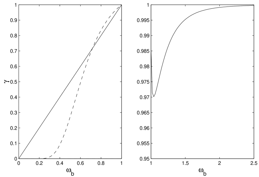
Figure 2: Some values of the symmetry coefficient $\gamma$. Left, soft on–site potentials: dashed line: $V(u_{n})=\frac{1}{2}u_{n}^{2}-\frac{1}{3}u_{n}^{3}$; continuous line: $V(u_{n})=\frac{1}{2}(\exp(-u_{n})-1)^{2}$. Right, hard on–site potential: $V(u_{n})=\frac{1}{2}u_{n}^{2}+\frac{1}{3}u_{n}^{3}+\frac{1}{4}u_{n}^{4}$. Rest frequency $\omega_{0}=1$.

6 Generalization

Theorems 1 and 2 are equally applicable if the system has inhomogeneities at the coupling matrix but not if they are at the on–site potential. Here we introduce the generalization to a broad class of Klein–Gordon systems, including different masses or inertia momenta, inhomogeneous on-site potentials with several minima, nonlinear coupling, solutions with different phases (i.e, not restricted to time–reversible solutions). Let us consider a Klein–Gordon system with Hamiltonian

$$H=\sum_{n}\left(\frac{1}{2}\,m_{n}\,\dot{u}_{n}^{2}\,+\,V_{n}(u_{n})\right)\,+\,\varepsilon\,W(u)\,,$$ (24)

and dynamical equations

$$m_{n}\,\ddot{u}_{n}\,+\,V_{n}^{\prime}(u_{n})\,+\,\varepsilon\,\frac{\partial W(u)}{\partial{u_{n}}}\,=\,0\,,$$ (25)

which at zero coupling become:

$$m_{n}\,\ddot{u}_{n}\,+\,V_{n}^{\prime}(u_{n})\,=\,0\,\quad\forall n\,.$$ (26)

Suppose we can label the solutions of these equations, with given frequency $\omega_{\mathrm{b}}$ and period $T$, with a code composed of an index for the site $n$, another index for the different minima and solutions (biperiodic, etc, different potential wells) $\sigma_{n}$, which can be different for each site. If we considering a periodic solution for the $n$–th equation , it can be written as a $2\,\pi$ periodic function $g_{n\,\omega_{\mathrm{b}}\,\sigma_{n}}(\omega_{\mathrm{b}}\,t+\alpha)$. Let us suppose that $g_{n\,\omega_{\mathrm{b}}\,\sigma_{n}}$ is chosen such that $\alpha=0$ corresponds to the time symmetric solution with $\dot{g}_{n\,\omega_{\mathrm{b}}\,\sigma_{n}}(0)=0$ and $g_{n\,\omega_{\mathrm{b}}\,\sigma_{n}}(0)>g_{n\,\omega_{\mathrm{b}}\,\sigma_{n}}(\pi)$. Therefore, the solutions of equations (26) are determined by the code $\{n,\sigma_{n},\alpha_{n}\}$. If we consider a given solution at the anticontinuous limit we can simply write it as $u=[u_{1}^{0},\dots,u_{N}^{0}]^{\dagger}$, but now, the $u_{n}^{0}$ are, in general, different, because of the particular multibreather solution $u$, whose stability we are interested in.

The characteristic equations for the Newton operator $\mathcal{N}_{\varepsilon}$ are given by:

$$(\mathcal{N}_{\varepsilon}\,\xi)_{n}\,\equiv\,m_{n}\,\ddot{\xi}_{n}\,+\,V_{n}^{\prime\prime}(u_{n})\,\xi_{n}\,+\,\varepsilon\,\sum_{m}\frac{\partial^{2}W(u)}{\partial u_{n}\,\partial u_{m}}\,\xi_{m}\,=\,E\,\xi_{n}\,$$ (27)

which to first order in $\varepsilon$ calculated at $\varepsilon=0$ lead to

$$(\mathcal{N}_{0}\,\xi)_{n}\,+\,\varepsilon\,(\tilde{\mathcal{N}}\,\xi)_{n}\,=\,(E_{0}\,+\,\varepsilon\,\lambda)\,\xi_{n}\,,$$ (28)

where:

$$(\mathcal{N}_{0}\,\xi)_{n}\, \equiv \,m_{n}\,\ddot{\xi}_{n}\,+\,V_{n}^{\prime\prime}(u^{0}_{n})\,\xi_{n}\,=\,E_{0}\,\xi_{n}\,,$$ (29)

$$(\tilde{\mathcal{N}}\xi)_{n}\, \equiv V^{\prime\prime\prime}(u_{n}^{0})\,u_{n,\varepsilon}\,\xi_{n}\,+\,\sum_{m}\,\frac{\partial^{2}W(u^{0})}{\partial u_{n}\,\partial u_{m}}\,\xi_{m}\,=\,\lambda\,\xi_{n}\,.$$ (30)

with $u_{n,\varepsilon}\,=\,\big{(}\frac{\displaystyle\partial u_{n}}{\displaystyle\partial\varepsilon}\big{)}_{\varepsilon=0}$. The first set of equations is the characteristic equation for the Newton operator at zero coupling, and the second one for the perturbation operator $\tilde{\mathcal{N}}$. The only periodic solution of each equation (29) with $E_{0}=0$ for a given solution $u_{0}$ of (26) , is $\dot{u}_{n}^{0}$. Thus, we can construct a ortonormal basis of $\ker(N_{0})$, restricted to periodic solutions (and, therefore, that can be chosen real) of given period $T$, as $|n\rangle\,=\,\frac{1}{\mu_{n}}[0,\dots,0,\dot{u}_{n}^{0},0,\dots,0]^{\dagger}$, with the only nonzero element at the $n$ position, and $\mu_{n}=\sqrt{\int_{-T/2}^{T/2}(\dot{u}_{n}^{0})^{2}\d t}$.

Deriving Eq. (25) with respect to $\varepsilon$ at $\varepsilon=0$ we get:

$$\big{(}\mathcal{N}_{0}\,\frac{\partial u}{\partial\varepsilon}\big{)}_{n}\,\equiv\,m_{n}\,\ddot{u}_{n,\varepsilon}\,+\,V_{n}^{\prime\prime}(u^{0}_{n})\,u_{n,\varepsilon}\,=\,-\,\sum_{m}\,\frac{\partial^{2}\,W(u^{0})}{\partial u_{n}\,\partial u_{m}}$$ (31)

Following exactly the same procedure as in section 3 we get the perturbation matrix $Q$, in extended form, with non diagonal elements for indexes corresponding to excited oscillators:

$$Q_{n\,m}\,=\,\langle n|\partial^{2}_{u\,u}W(u^{0})|m\rangle\,=\,\frac{1}{\mu_{n}\,\mu_{m}}\int_{-T/2}^{T/2}\,\dot{u}_{n}\frac{\partial^{2}W(u^{0})}{\partial u_{n}\,\partial u_{m}}\,\dot{u}_{m}\,\d\,t\,,\quad n\neq m\,\,$$ (32)

and diagonal elements

$$Q_{n\,n}=-\sum_{\forall\,m\neq n}\,\frac{\mu_{m}}{\mu_{n}}\,Q_{n\,m}\,.$$ (33)

If there are $p$ oscillators at rest and $N-p$ excited oscillators, the extended matrix $Q$ has $p$ zero columns and rows corresponding to the indexes of the oscillators at rest. The reduced form of $Q$ is the $N-p$ squared matrix, equal to $Q$ but stripped of those zero rows and columns. As a result we can establish the theorem:

Theorem 3 (Generalized MST)

Given a generalized Klein–Gordon system (24), a specific multibreather solution at zero coupling $\{u^{0}_{n}\}$, determined by a suitable set of codes, $u$ the corresponding solution at low coupling, $\{\lambda\}_{i=1}^{N-p}$ the eigenvalues of the reduced matrix $Q$, with only one zero, and being the wells corresponding to the $N-p$ specific $u^{0}_{n}$, of the same type, hard or soft, then:
The solution $u$ is stable if:
a) The on–site potentials are soft and there is not any positive value in $\{\varepsilon\,\lambda_{i}\}_{i=1}^{N-p}$.
b)The on–site potentials are hard and there is not any negative value in $\{\varepsilon\,\lambda_{i}\}_{i=1}^{N-p}$

This theorem includes both theorems 1 and 2. Certainly, it is of not so straightforward applicability, although for certain cases there are only a few matrix elements $Q_{n\,m}$ to calculate. As an example, if there are just two types of sites, the on–site potentials are symmetric, the coupling is linear and we consider only time–reversible multibreathers, there are only two different matrix elements to calculate.

7 Applications

7.1 Two–site breathers

A trivial example is the theorem about the stability of the two–site breather found in Ref. [5] page 69. Here we generalize it to non–symmetric on–site potentials. The coupling matrix corresponding to periodic boundary conditions and of the standard (spring–type) attractive form, has elements $C_{n\,m}\,=\,2\,\delta_{n\,m}-\delta_{|n-m|,1}$ and $C_{N\,1}\,=\,C_{1\,N}\,=\,-1$, that is:

$$C\,=\,\left[\begin{array}[]{rrrrrr}\;2&\;-1&0&\dots&\;0&\;-1\\ -1&2&-1&0&\dots&0\\ \dots&\dots&\dots&\dots&\dots&\dots\\ -1&0&\dots&0&-1&2\end{array}\right]\,.$$ (34)

If the two oscillator are in phase, the perturbation matrix is

$$Q\,=\,\left[\begin{array}[]{rr}\;1&\;-1\\ -1&1\end{array}\right]\,,$$

with eigenvalues $(\lambda_{1},\lambda_{2})=(0,2)$, the first one corresponds to the phase mode, the second to the antisymmetric eigenmode. Thus, one of the two bands tangent to the axis $E=0$ at zero coupling will remain there, and the other will move upwards. If the on–site potential is soft, i.e., with positive curvature, a intersection/tangent point will be lost, and the two site breather is unstable. For the hard on–site potential, the curvature of the bands is negative, and when the band moved upwards, the intersection points will be kept, and the system is be stable. If $\varepsilon<0$ the signs of the eigenvalues $\varepsilon\,E_{i}$ are reversed and so are the conclusions.

For the out–of–phase, two-site breather, with code $\sigma=[1,-1]$, the perturbation matrix is:

$$Q\,=\,\left[\begin{array}[]{rr}\;-\gamma&\;\gamma\\ \gamma&-\gamma\end{array}\right]\,,$$

with eigenvalues $(\lambda_{1},\lambda_{2})=(0,-2\gamma)$. The conclusions above are reversed, being the instability mode, when appropriate, the symmetric one. Note that the boundary conditions in $C$ have no effect.

Theorem 4 (Two–site breathers)

Consider time–reversible, two–site breathers in an homogeneous Klein-Gordon system with attractive linear coupling, then:
a) The two-site breathers with codes $\pm\,[1,1]$ and soft on–site potential are unstable and with $\pm\,[-1,1]$ are stable.
b) The two-site breathers with code $\pm\,[1,1]$ and hard on–site potential are stable and with $\pm\,[-1,1]$ are unstable.
c) If the coupling is repulsive, the conclusions are reversed.

7.2 Three–site breathers

Let us renumber the sites $1,2,3$ and suppose that the code of the site in the middle is $\sigma_{2},=\,+1$ as a reference, i.e., $\sigma\,=\,[\sigma_{1},1,\sigma_{3}]$. We define $\alpha_{i}=1$ if $\sigma_{i}=1$ and $\alpha_{i}=-\gamma$ if $\sigma_{i}=-1$, for $i=1,2$. Using $C$ from Eq. (34) the perturbation matrix is:

$$Q\,=\,\left[\begin{array}[]{rrr}\;\alpha_{1}&\;-\alpha_{1}&\;0\\ -\alpha_{1}&\;\alpha_{1}+\alpha_{3}&\;-\alpha_{3}\\ 0&\;-\alpha_{3}&\;\alpha_{3}\end{array}\right]\,.$$ (35)

Its nonzero eigenvalues are $\lambda_{\pm}\,=\,\alpha_{1}\,+\,\alpha_{3}\,\pm\,\sqrt{(\alpha_{1}\,+\,\alpha_{3})^{2}\,-\,3\,\alpha_{1}\,\alpha_{3}}$. In order to have both eigenvalues with the same sign, we need that $\alpha_{1}\,\alpha_{3}>0$, i.e., either $\alpha_{3}\,=\,\alpha_{1}\,=\,1$, or $\alpha_{3}\,=\,\alpha_{1}\,=\,-\gamma$. That is, if $\sigma_{1}=\sigma_{3}=1$, $\lambda_{\pm}=1,3>0$, if $\sigma_{1}=s_{3}=-\gamma$, $\lambda_{\pm}=-\gamma,-3\gamma<0$, and if $\sigma_{1}\,\sigma_{2}=-1$, then $\lambda_{\pm}$ have different signs. Therefore:

Theorem 5 (Three–site breathers)

Consider time–reversible, three–site breathers in an homogeneous K-G system with nearest–neighbor, linear coupling, attractive for $\varepsilon>0$. Then:
a) The three–site breathers with codes $\sigma\,=\,\pm[-1,1,-1]$ are stable if $\varepsilon>0$ ($\varepsilon<0$)and the on–site potential is soft (hard).
b) The three–site breathers with code $\sigma\,=\,\pm[1,1,1]$ are stable if $\varepsilon>0$ $(\varepsilon<0)$ and the on–site potential is hard (soft).
c) All other three-site breathers are unstable for any sign of $\varepsilon$ and type of on–site potential.

We can compare the predictions of the values given by the theory with the numerically calculated values of the intersection points of the bands with the axis $\theta=0$. As an example, the numerically calculated eigenvalues and the predictions given by theorems 1 and 2 for the three–site breather with code $[-1,1,-1]$ are plotted in Figure 3. The very good accuracy is evident.

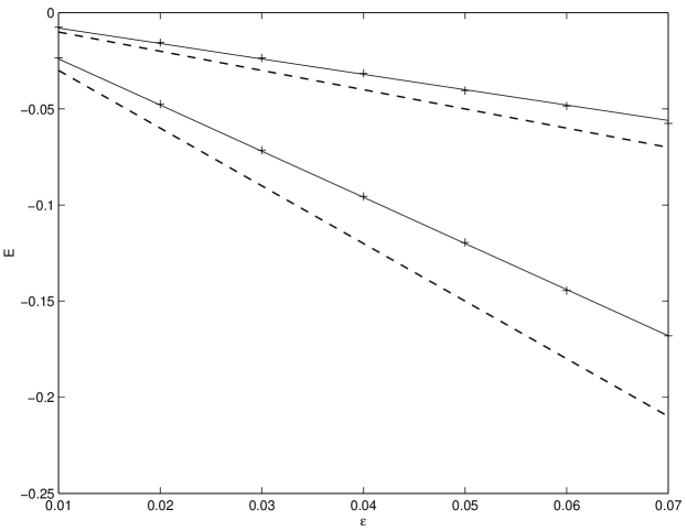
Figure 3: Comparison between the eigenvalues $E$ of the Newton operator obtained numerically (points), predicted by the symmetric MST, theorem 1, (dashed lines) and by the non–symmetric MST, theorem 2, (continuous line), which is the right one to be used. Morse potential, code $[-1,1,-1]$, frequency $\omega_{\mathrm{b}}=\gamma=0.8$.

7.3 A model with long–range interaction

An example of system with long range interaction is the twist model used in Ref. [9]. The dynamical equations are:

$$\ddot{u}_{n}\,+\,V^{\prime}(u_{n})+\varepsilon\sum_{m=n-N/2}^{n+N/2}\frac{\cos[\theta_{tw}(n-m)]}{|n-m|^{3}}\;u_{m}=0\,$$ (36)

$V$ being the Morse potential, and $\theta_{tw}$ the angle between two dipole moments corresponding to neighboring base pairs in a simplified model of DNA. The coupling matrix elements are:

$$C_{n\,m}=\frac{\cos[\theta_{tw}(n-m)]}{|n-m|^{3}}\;,$$ (37)

Some of the results, also checked numerically and with good accuracy with respect to the eigenvalues $E$, given by theorem 1, in spite of $V$ being non–symmetric are:

Code	$\theta_{tw}=0$	$\theta_{tw}=\pi$
11	Stable	Unstable
1 -1	Unstable	Stable
101	Stable	Stable
111	Stable	Unstable
1-1 1	Unstable	Stable
11-1	Unstable	Stable

As an example of the effect of the symmetry coefficient $\gamma$ in theorem 2, we can consider the code $[1,-1,1]$ and plot the Newton eigenvalues $E$ as a function of $\theta_{tw}$. The perturbation matrix is:

$$Q=\,\left[\begin{array}[]{ccc}\;\gamma a-b&\;\;-\gamma a&b\\ -\gamma a&\;\;2\gamma a&-\gamma a\\ b&\;\;-\gamma a&\;\;\gamma a-b\end{array}\right]\;,$$ (38)

with $a=\cos(\theta_{tw})$ and $b=\cos(2\theta_{tw})/8$. Figure 4 shows the dependence of the eigenvalues $\lambda$ on the twist angle $\theta_{tw}$ for three values of the symmetry coefficient $\gamma$. It can be seen that only values of $\gamma$ very far from $1$ lead to a change on the stability prediction.

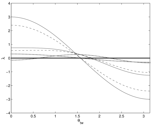
Figure 4: Eigenvalues $\lambda$ of the perturbation matrix $Q$ for a three-site breather with code $[-1,1,-1]$ on the twist model. Continuous line: $\gamma=\omega_{\mathrm{b}}=1$; dashed line: $\gamma=\omega_{\mathrm{b}}=0.8$; and dotted line: $\gamma=\omega_{\mathrm{b}}=0.1$. Only values of $\gamma$ very far from $1$ lead to a different stability prediction.

8 Multibreathers, phonobreathers and dark breathers. Parity instabilities.

For larger, time–reversible multibreathers in homogeneous Klein–Gordon systems with nearest–neighbor, linear coupling, it is trivial to obtain the stability properties of the two different solutions with wave number $q=0$, all the oscillators in phase, or $q=\pi$, neighboring oscillators out of phase. Consider any number $N^{\prime}$ of contiguous oscillators in phase in a system coupled by the matrix $C$ in Eq. (34). The $N^{\prime}\,\times\,N^{\prime}$ perturbation matrix is given by:

$$Q\,=\,\left[\begin{array}[]{rrrrrr}\;1&\;-1&\;0&\dots&\;0&\;0\\ -1&2&-1&0&\dots&0\\ \dots&\dots&\dots&\dots&\dots&\dots\\ 0&0&\dots&-1&2&-1\\ 0&0&\dots&0&-1&1\end{array}\right]\,.$$ (39)

The characteristic equation for $Q\,x=\lambda\,x$ corresponds to the following equations:

$$x_{1}\,-\,x_{2}\, = \,\lambda\,x_{1}\,,$$

$$2x_{n}\,-\,x_{n+1}\,-\,x_{n-1}\, = \,\lambda\,x_{n},\quad\forall\,n\,\neq\,1,2\,,$$

$$x_{N^{\prime}}\,-\,x_{N^{\prime}-1}\, = \,\lambda\,x_{N^{\prime}}\,.$$ (40)

Substitution of the trial solution $x_{n}=\cos(q\,n-\phi_{q})$, leads to $\phi_{q}=q/2$, $q=m\,\pi/N^{\prime}$, with $m=0,\dots,N^{\prime}-1$, and $\lambda_{m}=4\,\sin^{2}(m\,\pi/(2\,N^{\prime}))$, i.e., positive eigenvalues without a degenerate zero. In case all the oscillators of the group are out of phase, $Q\rightarrow-\gamma Q$ and $\lambda_{m}\rightarrow-\gamma\lambda_{m}$. Therefore:

Theorem 6

If $\varepsilon>0$, the time–reversible, in-phase, multibreathers are unstable (stable) with soft (hard) on–site potential. For any out–of–phase multibreathers, and $\varepsilon<0$ the conclusions are reversed.

Although, we have no mathematical proof, according to numerical calculations of the eigenvalues of the perturbation matrices corresponding to groups with different codes, the numbers of negative and positive eigenvalues are equal to the numbers of $-1$ and $+1$ in $\{\sigma_{n}\,\sigma_{n+1}\}_{n=1}^{N^{\prime}-1}$. Therefore being unstable for any on–site potential.

Note that if there are several non–contiguous multibreathers, the perturbation matrix if composed of independent blocks of perturbation submatrices of the same type, each one with a zero eigenvalue by construction as seen in subsection 4.1. The stability of such a system cannot be determined by the MST. The only possible conclusion is that if there are eigenvalues of different sign this system would be unstable.

Phonobreathers are multibreathers without oscillators at rest. For time–reversible phonobreathers in a system either with free–ends, or fixed-ends boundary conditions, the perturbation matrix $Q$ is the same as in Eq. (39). If the boundary conditions are periodic, the only change is that $Q_{1\,1}=Q_{N,N}=2$, $Q_{N\,1}=Q_{1,N}=-1$, and the eigenvalues are the same. That is, the mode $q=0$ with attractive coupling and hard potential is stable. Changing the hardness, the type of coupling, or the mode, changes each time the stability. In this way, we reproduce the results in Refs. [7, 6] as a consequence of modulational instability and using the DNLS approximation, respectively, and in theorem 9 in Ref. [3], based in the properties of the action.

Parity instabilities are a interesting effect for phonobreathers with periodic boundary conditions. It is a consequence of the parity of the total number of sites $N$. If, for example, $V$ is soft, the coupling is attractive, and $N$ is even, all the eigenvalues of the perturbation matrix are negative, i.e., the system is stable. But if $N$ is odd, there is an isolated positive eigenvalue, bringing about the instability. There is a clear physical origin of this phenomenon, as the boundaries are equivalent to an inhomogeneity. According to our theory it is also obvious: we have, in fact two oscillators at the ends coupled and in phase, which gives rise to a positive eigenvalue.

Dark breathers are multibreathers with only one or a few oscillators at rest. Their stability depends on the characteristics of the contiguous groups of excited oscillators, as a consequence of theorem 6. We have to be careful about the number of particles, for example the $\pi$ mode with code around the dark site $[\dots,1,-1,0,1,-1,\dots]$, needs an odd number of sites to avoid having two in–phase oscillators at the ends, and a parity instability. The one with $[\dots,-1,1,0,1,-1,\dots]$ needs an even number of sites. If the system has free of fixed periodic conditions, the perturbation matrix is decoupled in two and the stability is undefined as commented above.

We have compared the predictions of the instabilities and the values of the intersection points of the bands with the axis $\theta=0$, in many cases, as for example in Ref. [10], with very good results. The question of up to which values of the coupling parameter $\varepsilon$ the theory is valid, is however unsolved. Generically speaking values up to $\varepsilon=0.1$ (compared to the rest frequency $\omega_{0}=1$), are safe, but there are some exceptions. In the same reference, for the dark breather hard on–site potential and attractive coupling, a mode not predicted by the MST gives rise to an instability as soon as $\varepsilon=0.022$.

As the width of the phonon band can be calculated, and the width of the background is given by the eigenvalues of the perturbation matrices, it is also possible to predict the values of the $\varepsilon$, for which oscillatory and subharmonic instabilities occur, but we do not extend further here.

9 Summary and conclusions

We have developed using degenerate perturbation theory a method for obtaining the stability properties of multibreathers of any code at low coupling. The method is synthesized in three different versions of a theorem, referred to as the multibreather stability theorem or MST for short. The two simplest versions correspond to time–reversible multibreathers, with linear coupling and homogeneous on–site potentials. If the on–site potential is symmetric or we consider only in–phase multibreathers, it involves only some simple modifications of the coupling matrix. If none of those conditions are fulfilled then it involves the analytical or numerical calculations of a magnitude $\gamma$, called the symmetry coefficient, as its value is $1$ for symmetric on–site potentials. For soft potentials and values of the frequency until about one half of the rest frequency, a good approximation is the multibreather frequency, result which we demonstrate is exact for the Morse potential. For hard potentials its value its close to unity. The generalized version of the MST is of not so straightforward applicability, although its complexity depends on the characteristics of the system and multibreather considered.

We give some examples of application of the method and compare it with numerical results. The systems considered are two and three–site breathers, with nearest neighbor or long–range interactions, multibreathers, phonobreathers and dark breathers. A parity instability can appear in finite systems depending on the parity of the number of oscillators. All these examples are interesting in themselves, but also illustrate the use of the MST, and show that it provides a powerful method of easy applicability to determine multibreathers stability.

Some other applications under study are multibreathers in 2D and 3D systems, prediction of the oscillatory and subharmonic instabilities and the peculiarities of some disordered systems

Appendix A Calculation of the symmetry parameter $\gamma$ for a Morse potential

In this appendix, we calculate the value of the symmetry parameter $\gamma$ in theorem 2 for the particular case of a Morse potential. The choice of this kind of potential relies in the fact that the expressions of the orbits are easy to manage. We will proof that, for this potential, $\gamma=\omega_{\mathrm{b}}$.

Let us suppose an isolated oscillator submitted to a Morse potential. The energy of the system is:

$$\mathcal{E}=\frac{1}{2}\dot{x}^{2}+\frac{1}{2}(\exp(-x)-1)^{2}\,.$$ (41)

We look for solutions with period $T=2\pi/\omega_{\mathrm{b}}$ that are time–reversible, i.e, with $\dot{x}(0)=0$, or, in other words, at $t=0$ the system is at a turning point. There are two of them, obtained from the equation above: $x_{1}=-\log(1+\sqrt{2\,\mathcal{E}})<0$ and $x_{2}=-\log(1-\sqrt{2\,\mathcal{E}})>0$. If we consider the solution with $x(0)=x_{1}$, t(x) is given by:

$$t(x)=\int_{x_{1}}^{x}\frac{\mathrm{d}x}{\sqrt{2(\mathcal{E}-(\exp(-x)-1)^{2}/2)}}\;,$$ (42)

which leads to:

$$t(x)=\frac{1}{\sqrt{1-2\,\mathcal{E}}}\left(\frac{\pi}{2}-\arcsin\big{[}\frac{1}{\sqrt{2\,\mathcal{E}}}\;\big{(}1+\frac{2\,\mathcal{E}-1}{\exp(-x)}\;\big{)}\big{]}\right)\,.$$ (43)

By substitution of $t=T/2=\pi/\omega_{\mathrm{b}}$ and $x=x_{2}$ we obtain $\omega_{\mathrm{b}}=\sqrt{1-2\,\mathcal{E}}$.

The inversion of Eq. (42) leads to:

$$x(t)=\log\frac{1-\sqrt{1-\omega_{\mathrm{b}}^{2}}\cos\omega_{\mathrm{b}}\,t}{\omega_{\mathrm{b}}^{2}}\,.$$ (44)

To calculate $\gamma$, we need the Fourier coefficients of $x(t)$. If the solution $x(t)$ is expressed as:

$$x(t)=z_{0}+2\sum_{k=1}^{\infty}z_{k}\cos(k\,\omega_{\mathrm{b}}\,t)\;,$$ (45)

the coefficients $\{z_{k}\}_{k=0}^{\infty}$ are given by:

$$z_{k}=\frac{1}{T}\int_{-T/2}^{T/2}x(t)\cos(k\,\omega_{\mathrm{b}}\,t)\d t\,.$$ (46)

The calculation of these integrals is straightforward and leads to:

$$z_{0}=\log\frac{\displaystyle 1+\omega_{\mathrm{b}}}{\displaystyle 2\omega_{\mathrm{b}}^{2}}\quad;\quad z_{k}=-\,\frac{\displaystyle 1}{\displaystyle n}\Big{(}\;\frac{\displaystyle 1-\omega_{\mathrm{b}}}{\displaystyle\sqrt{1-\omega_{\mathrm{b}}^{2}}}\;\Big{)}^{k}\,.$$ (47)

The parameter $\gamma$ is given by:

$$\gamma=-\frac{\sum_{k\geq 1}(-1)^{k}k^{2}z_{k}^{2}}{\sum_{k\geq 1}k^{2}z_{k}^{2}}.$$ (48)

By substitution of the Fourier coefficients in Eq. (47), we obtain

$$\gamma=-\frac{\sum_{k\geq 1}(-r)^{k}}{\sum_{k\geq 1}r^{k}}\,\quad\textrm{with}\quad r=\frac{1-\omega_{\mathrm{b}}}{1+\omega_{\mathrm{b}}}\,.$$ (49)

As $|r|<1$, $\gamma$ can be easily calculated using the expressions for the sum of an infinite geometric progression:

$$\sum_{k\geq 1}r^{k}=\frac{\displaystyle r}{\displaystyle 1-r}\quad,\quad\sum_{k\geq 1}(-r)^{k}=-\frac{\displaystyle r}{\displaystyle 1+r}$$ (50)

leading to $\gamma=\omega_{\mathrm{b}}$, as we wanted to proof.

Appendix B Curvature of the bands

In this section we demonstrate a key point used in our theory: the fact that the band corresponding to an isolated excited oscillators has negative curvature if the on site potential is hard and positive if it is soft. Unfortunately, the demonstration is quite long if we want it to be self–consistent. A similar one can be found in Ref. [11] and different ones in Ref. [5, 12].

Let us consider the dynamical equation of an isolated oscillator with Hamiltonian $H=1/2\,p^{2}+V(u)$, with $u$ a single–value, real function of time and $p=\dot{u}$:

$$\ddot{u}+V^{\prime}(u)=0\,$$ (51)

The characteristic equation for the Newton operator $\mathcal{N}$ corresponding to a given periodic solution of Eq. (51)is

$$\mathcal{N}\xi\equiv\ddot{\xi}+V^{\prime\prime}(u)\xi=E\xi\,,$$ (52)

where $\xi$ is a $\mathcal{C}^{2}$ function of $t$. For each eigenvalue $E$ there are only 2 independent solutions, determined, for example, by the values of $\xi(0)$ and $\dot{\xi}(0)$. We can obtain them for $E=0$, by deriving Eq. (51) with respect to $t$ and with respect to $\omega_{\mathrm{b}}$:

$$\dddot{u}+V^{\prime\prime}(u)\dot{u}=0\Leftrightarrow\mathcal{N}\dot{u}=0\quad;\quad\ddot{u}_{w}+V^{\prime\prime}(u)u_{w}=0\Leftrightarrow\mathcal{N}u_{w}=0\,.$$ (53)

As we have a single oscillator we can suppose that $u(t)$ is time symmetric with a suitable origin of time, i.e., $\dot{u}$ is a time-antisymmetric function of $t$ with the same period $T=2\,\pi/\omega_{\mathrm{b}}$ as $u(t)$: $\dot{u}(t+T)=\dot{u}(t)$, $\dot{u}(0)=\dot{u}(T)=0$. The properties of $u_{w}=du/d\omega_{\mathrm{b}}$, can be also obtained. We can write $u$ as a cosine Fourier series $u(t)=\sum_{k=0}^{\infty}c_{k}\cos(\omega_{\mathrm{b}}\,t)$, with the coefficients $c_{k}$ depending on $\omega_{\mathrm{b}}$. Therefore, ${du}/{d\omega_{\mathrm{b}}}=\sum_{k=0}^{\infty}(dc_{k}/d\omega_{\mathrm{b}})\cos(\omega_{\mathrm{b}}\,t)+\sum_{k=0}^{\infty}-k\,t\sin(\omega_{\mathrm{b}}\,t)$, or:

$$u_{w}\equiv\frac{du}{d\omega_{\mathrm{b}}}=\gamma(t)+\frac{t}{\omega_{\mathrm{b}}}\,\dot{u}(t)\,$$ (54)

$\gamma(t)$ being a time symmetric, periodic function of time with the same period $T$ as $u$. This functions constitute a base of the eigenspace corresponding to $E=0$.

On the other hand, $\mathcal{N}$ (52) is a periodic operator because it depends on a periodic function $u$. Its eigenfunctions are given by the Bloch theorem:

$$\xi(\theta,t)=\chi(\mathrm{i}\theta,t)\exp(\theta t/T),$$ (55)

with $\chi$ a T–periodic function of time and $\theta=\theta(E)$. If we consider only values of $E$ for which $\theta$ is real, the set of points $(\theta,E(\theta)$ constitutes a band. If $\xi$ is a solution of $\mathcal{N}\,\xi=E\xi$, the fact that $\mathcal{N}$ is a real operator implies that $\xi^{*}$ is another solution, i.e., $(-\theta,E)$ also belongs to the band and this is symmetric with respect to $\theta$ and, therefore, $\d E/\d\theta(0)=0$. As $\mathcal{N}$ is time–symmetric $\xi(\theta,-t)$ is another, and has to be proportional to $\xi^{*}$ as there can be only two independent solutions.

The Floquet matrix $F_{E}$ is defined as:

$$\left[\begin{array}[]{c}\xi(T)\\ \dot{\xi}(T)\end{array}\right]=F_{E}\left[\begin{array}[]{c}\xi(0)\\ \dot{\xi}(0)\end{array}\right]\,.$$ (56)

The eigenvalues $\{\lambda_{l}\}$ of $F_{E}$ are the Floquet multipliers, if we write them as $\lambda_{l}=\exp{\mathrm{i}\theta_{l}}$, with $\theta$ real or complex, $\mathrm{i}\theta_{l}$ are the Floquet exponents, and $\theta_{l}$, the Floquet arguments. An eigenfunction with $\theta_{l}$ real is bounded, if $\theta_{l}=1$ the eigenfunction has period $T$. The condition for linear stability of the solution $u$ is that all the Floquet arguments of $F_{0}$ are real.

It is easy to check some properties. The Bloch functions Eq. (55) are eigenfunctions of $F_{E}$ with Floquet exponent $\theta$, therefore $F_{E}$ is diagonalizable (over $\mathcal{C}$) with Floquet multipliers $\exp(\pm\mathrm{i}\theta)$ and Floquet arguments $\pm\theta$. However, at $E=0$, there is only one eigenfunction of $F_{0}$, $\dot{u}$, the other independent function of the subspace $\mathcal{N}\,\xi=0$, $u_{w}$, it is not an $F_{0}$–eigenfunction. That is $F_{0}$ has a degenerate Floquet multiplier $1$, or Floquet argument $0$ and can be transformed into a Jordan block. Another consequence of the latter is that $(\theta,E)=(0,0)$ belongs to the band. We need to calculate the curvature of the band at this point.

Let us come back to the Bloch functions $\xi(\theta,t)$ in Eq. (55) and $\xi^{*}(\theta,t)$ corresponding to a pair of symmetric points $(\pm\theta,E)$ of the band, and suppose that $\theta\rightarrow 0$ (and then $E\rightarrow 0$). At $\theta=0$ the two functions collide in $\xi(0,t)=\chi(0,t)=\chi^{*}(0,t)$, therefore $\xi(0,t)$ is a real, $T$–periodic function. But we already now that at $E=0$, there is a $T$–periodic function solution of $\mathcal{N}\,\xi=0$, $\dot{u}$. Therefore, $\xi(0,t)=\dot{u}$ ($\mathcal{N}$ is lineal, so we can adjust the norm of $\xi$ in order that the latter equation is fulfilled).

We can reobtain the missing function that spans $\ker(\mathcal{N})$. If we derive Eq. (52) with respect to $\theta$, we obtain $\mathcal{N}\,\xi_{\theta}=E_{\theta}\xi+E\xi_{\theta}$ and at $E=0$ ($E_{\theta}(0)=0$) we obtain: $\mathcal{N}\,\xi_{\theta}(0,t)=0$. Deriving $\xi(\theta,t)$ in Eq. (55) we get:

$$\xi_{\theta}=\chi_{\theta}(\theta,t)\exp(\mathrm{i}\theta/T)+\mathrm{i}\frac{t}{T}\chi(\theta,t)\exp(\mathrm{i}\theta/T)=\chi_{\theta}\exp(\mathrm{i}\theta/T)+\mathrm{i}\frac{t}{T}\xi\,.$$ (57)

At $\theta=0$, $\xi=\dot{u}$ and $\xi_{\theta}$ has to be proportional at $u_{w}$, which we know is the other independent function. Therefore

$$\xi_{\theta}(0,t)=\chi_{\theta}+\mathrm{i}\frac{t}{T}\,\dot{u}=\mathrm{i}\frac{\omega_{\mathrm{b}}}{T}\,\left(\frac{T}{\mathrm{i}\omega_{\mathrm{b}}}\,\chi_{\theta}+\frac{t}{\omega_{\mathrm{b}}}\,\dot{u}\right)=\mathrm{i}\frac{\omega_{\mathrm{b}}^{2}}{2\pi}\,\left(-\frac{2\pi}{\omega_{\mathrm{b}}^{2}}\,\chi_{\theta}+\frac{t}{\omega_{\mathrm{b}}}\,\dot{u}\right)\,.$$

Comparing with Eq. (54) we obtain

$$\xi_{\theta}(0,t)=\mathrm{i}\frac{\omega_{\mathrm{b}}^{2}}{2\pi}\,u_{w}.$$ (58)

The following step is to express the curvature $E_{\theta\theta}$ of the band $E(\theta)$ at $(\theta,E)=(0,0)$ in terms of $u$ and its derivatives. Let us derive Eq. (52) twice with respect to $\theta$, we obtain:

$$\mathcal{N}\,\xi_{\theta\theta}=E_{\theta\theta}\,\xi+2\,E_{\theta}\,\xi_{\theta}+E\,\xi_{\theta\theta}\Rightarrow\mathcal{N}\,\xi_{\theta\theta}=E_{\theta\theta}\,\dot{u}\quad\mathrm{at}\,\,\theta=0\,.$$ (59)

Multiplying to the right by $\dot{u}$ and integrating a period we get

$$E_{\theta\theta}\,\int_{t=0}^{T}\dot{u}^{2}\d t=\int_{t=0}^{T}\dot{u}\mathcal{N}\,\xi_{\theta\theta}\d t\,.$$ (60)

For any pair of functions $f(t)$ and $g(t)$

$$\int_{t=0}^{T}f\mathcal{N}\,g = \int_{t=0}^{T}(f\,\ddot{g}+f\,V^{\prime\prime}\,g)\d t=[f\,\dot{g}]_{t=0}^{T}-[\dot{f}\,g]_{t=0}^{T}+\int_{t=0}^{T}(g\ddot{f}+g\,V^{\prime\prime}\,g)\,dt$$

$$= [f\,\dot{g}]_{t=0}^{T}-[\dot{f}\,g]_{t=0}^{T}+\int_{t=0}^{T}g\,\mathcal{N}\,f\d t\,.$$

Applying the latter equation:

$$\int_{t=0}^{T}\dot{u}\mathcal{N}\,\xi_{\theta\theta}\d t=[\dot{u}\,\dot{\xi}_{\theta\theta}]_{t=0}^{T}-[\ddot{u}\,\xi_{\theta\theta}]_{t=0}^{T}+\int_{t=0}^{T}(\xi_{\theta\theta}\,\mathcal{N}\,\dot{u})\d t\,.$$ (61)

Using that $\mathcal{N}\,\dot{u}=0$, $\dot{u}(0)=\dot{u}(T)=0$ and $\ddot{u}(0)=\ddot{u}(T)$ the previous equation leads to

$$\int_{t=0}^{T}\dot{u}\,\mathcal{N}\,\xi_{\theta\theta}\d t=-\ddot{u}(T)\left(\xi_{\theta\theta}(0,T)-\xi_{\theta\theta}(0,0)\right)\,.$$ (62)

To calculate the last difference, let us derive Eq. (57) with respect to $\theta$. We obtain

$$\xi_{\theta\theta} = \chi_{\theta\theta}\exp(\mathrm{i}\theta t/T)+\mathrm{i}\frac{t}{T}\,\chi_{\theta}\exp(\mathrm{i}\theta t/T)+\mathrm{i}\frac{t}{T}\,\xi_{\theta}$$

$$= \chi_{\theta\theta}\exp(\mathrm{i}\theta t/T)+\mathrm{i}\frac{t}{T}\,(\xi_{\theta}-\mathrm{i}\frac{t}{T}\,\xi)+\mathrm{i}\frac{t}{T}\,\xi_{\theta}$$

$$= \chi_{\theta\theta}\exp(\mathrm{i}\theta t/T)+2\mathrm{i}\frac{t}{T}\,\xi_{\theta}+\frac{t^{2}}{T^{2}}\xi$$

$$\Rightarrow \quad\xi_{\theta\theta}=\chi_{\theta\theta}+2\mathrm{i}\frac{t}{T}\,\xi_{\theta}+\frac{t^{2}}{T^{2}}\dot{u}\quad\mathrm{at}\,\,\,\theta=0\,.$$

$\chi$ and therefore $\chi_{\theta\theta}$ are $T$–periodic functions, therefore $\xi_{\theta\theta}(0,0)=\chi_{\theta\theta}(0,0)=\chi_{\theta\theta}(0,T)$ and $\xi_{\theta\theta}(0,T)-\xi_{\theta\theta}(0,0)=2\mathrm{i}\,\xi_{\theta}(0,T)\,.$ Then

$$\int_{t=0}^{T}\dot{u}\,\mathcal{N}\,\xi_{\theta\theta}\d t=-\ddot{u}\,(2\mathrm{i}\xi_{\theta}(0,T))=\frac{\partial H}{\partial u(T)}\,2\mathrm{i}\,(\mathrm{i}\frac{\omega_{\mathrm{b}}^{2}}{2\pi}\,u_{w}(T))=-\frac{\omega_{\mathrm{b}}^{2}}{\pi}\frac{\d H}{\d\omega_{\mathrm{b}}}\,.$$

Substituting in Eq. (60), and naming the action $I=\int_{t=0}^{T}\dot{u}^{2}\,\d t$ we finally obtain at $\theta=0$:

$$E_{\theta\theta}(0)=-\frac{\omega_{\mathrm{b}}^{2}}{\pi I}\,\frac{\d H}{\d\omega_{\mathrm{b}}}\,.$$ (63)

$I$ is always positive, therefore, if the potential is hard ($\d H/\d\omega_{\mathrm{b}}>0$), the curvature $E_{\theta\theta}$ is negative and the band is tangent to the axis $E=0$ from below, if it is soft ($\d H/\d\omega_{\mathrm{b}}<0$) the curvature is positive and the band is tangent form above, as we wanted to demonstrate.

Note that this demonstration is also valid for the whole coupled system with the obvious changes: $u\rightarrow[u_{1},\dots,u_{N}]^{\dagger}$; $V(u)\rightarrow V(u)+\varepsilon W(u)$, $W(u)$ being the coupling potential; $V^{\prime}(u)\rightarrow[\partial V/\partial u_{1},\dots,\partial V/\partial u_{N}]^{\dagger}$; $V^{\prime\prime}(u)$ the matrix with elements $\partial^{2}V/\partial u_{n}\partial u_{m}$ and analogously. We also need the additional constraint that the solution $u(t)$ is chosen time–symmetric and that the pair of eigenvalues with $\theta=0$ is isolated. This means that the band tangent at $(\theta,E)=(0,0)$ continues having the same curvature properties depending on the hardness/softness of the potential

References

- [1] RS MacKay and S Aubry. Proof of existence of breathers for time-reversible or Hamiltonian networks of weakly coupled oscillators. Nonlinearity, 7:1623–1643, 1994.
- [2] JL Marín and S Aubry. Breathers in nonlinear lattices: Numerical methods based on the anti–integrability concept. In L Vázquez, L Streit, and VM Pérez-García, editors, Nonlinear Klein–Gordon and Schrödinger Systems: Theory and Applications, pages 317–323. World Scientific, Singapore and Philadelphia, 1995.
- [3] S Aubry. Breathers in nonlinear lattices: Existence, linear stability and quantization. Physica D, 103:201–250, 1997.
- [4] S Flach and CR Willis. Discrete breathers. Physics Reports, 295:181–264, 1998.
- [5] JL Marín. Intrinsic Localised Modes in Nonlinear Lattices. PhD thesis, University of Zaragoza, Department of Condensed Matter, June 1997.
- [6] AM Morgante, M Johansson, G Kopidakis, and S Aubry. Standing waves instabilities in a chain of nonlinear coupled oscillators. Phys. D, 162:53, 2002.
- [7] I. Daumont, T. Dauxois, and M. Peyrard. Modulational instability: fisrt step towards energy localization in nonlinear lattices. Nonlinearity, 10:617–630, 1997.
- [8] D Griffiths. Introduction to Quantum Mechanics. Prentice Hall, New Jersey, USA, 1995.
- [9] B Sánchez-Rey, JFR Archilla, F Palmero, and FR Romero. Breathers in a system with helicity and dipole interaction. Phys. Rev. E, 66:017601–017604, 2002.
- [10] A Alvarez, JFR Archilla, J Cuevas, and FR Romero. Dark breathers in Klein-Gordon lattices. band analysis of their stability properties. New Journal of Physics, 4:72.1–72.19, 2002.
- [11] T Cretegny. Dynamique collective et localisation de l’énergie dans les reseaux non-linéaires. PhD thesis, École Normale Supérieure de Lyon, 1998.
- [12] G Kopidakis and S Aubry. Intraband discrete breathers in disordered nonlinear systems I: Delocalization. Physica D, 130:155–186, 1999.